
An FPTAS for Dynamic Multiobjective Shortest Path Problems


1
Network Optimization Department, Zuse Institute Berlin, Takustraße 7, 14195 Berlin, Germany
2
Departamento de Matemáticas, Estadística e Investigación Operativa, Universidad de La Laguna, 38271 San Cristóbal de La Laguna, Santa Cruz de Tenerife, Spain
*
Author to whom correspondence should be addressed.
Algorithms 2021, 14(2), 43; https://0-doi-org.brum.beds.ac.uk/10.3390/a14020043
Submission received: 30 November 2020
/
Revised: 15 January 2021
/
Accepted: 22 January 2021
/
Published: 29 January 2021
(This article belongs to the Special Issue Algorithms for Shortest Paths in Dynamic and Evolving Networks)
Abstract
:The Dynamic Multiobjective Shortest Path problem features multidimensional costs that can depend on several variables and not only on time; this setting is motivated by flight planning applications and the routing of electric vehicles. We give an exact algorithm for the FIFO case and derive from it an FPTAS for both, the static Multiobjective Shortest Path (MOSP) problems and, under mild assumptions, for the dynamic problem variant. The resulting FPTAS is computationally efficient and beats the known complexity bounds of other FPTAS for MOSP problems.
1. Introduction
We consider in this paper the solution of the Dynamic Multiobjective Shortest Path (Dyn-MOSP) problem that generalizes the standard shortest path problem in two ways. First, each arc of the graph bears more than one attribute (e.g., length, duration, consumption...); this produces the (static) Multiobjective Shortest Path (MOSP) problem. Second, generalizing arc attributes to functions gives rise to the Dyn-MOSP problem. In it, each arc function is evaluated along a path in a dynamic (programming) fashion, i.e., a time dependent function is evaluated based on passed time, a consumption dependent function based on resource consumption etc. We will refer to all arc and path attributes simply as cost. The goal in MOSP problems and Dyn-MOSP problems is then to find paths from a source node to all other nodes in the input graph that are minimal w.r.t. their costs.
Our setting is motivated by Flight Planning Problems (FPP), in which optimal aircraft routes have to be determined in an airway network, considering multiple and dynamic optimization criteria. The most important scenario is the simultaneous minimization of flight time and fuel consumption. The flight time depends on the weather, in particular, the wind, which changes over time and hence depends on the flight time itself. Similarly, the fuel consumption depends on the weight of the aircraft and hence, again, on the consumption so far. Another application with similar dynamics is the routing of electric vehicles through mountainous terrains with varying traffic congestion. Here, the traffic depends on the time of day, and the battery’s state of (dis)charge is non-linear.
In multiobjective optimization it is common to refer to optimal solutions using the terms efficient or Pareto optimal. Already the static MOSP problem is known to be intractable because of the possibly exponential cardinality of the solution set that, in this case, contains so called efficient paths (cf. Hansen [1]). This intrinsic difficulty of all multiobjective optimization problems can be circumvented by restricting attention to a polynomially sized subset of efficient solutions with an a priori bound on the quality loss w.r.t. the complete solution set. This idea lead to the development of Fully Polynomial Time Approximation Schemes (FPTAS) for MOSP problems in recent years (cf. Tsaggouris and Zaroliagis [2], Breugem et al. [3], or Bökler and Chimani [4]).
Our aim in this paper is to show that recently developed exact algorithms for MOSP problems can be generalized to also solve Dyn-MOSP instances, given that the arc cost functions fulfill the First In First Out (FIFO) property, i.e., a worse arrival at an arc’s tail node never turns out to be beneficial. We then introduce a new FPTAS for MOSP problems. For ease of exposition, we first consider the static case for which—to the best of our knowledge—it features the currently best asymptotic run time. Afterwards, we show that our results carry over to Dyn-MOSP problems if a certain (realistic) assumption on the arc cost functions is made. As usual in the FIFO setting, the asymptotic run time is the same as that of the static version. We finally provide extensive computational evidence of the efficiency of our approach. Indeed, our FPTAS is faster than existing ones for MOSP problems. Moreover and contrary to what was observed in the computational experiments presented in recent publications about FPTAS for static MOSP problems, the new FPTAS avoids the computation of a considerable number of paths in the dynamic costs setting.
1.1. Literature Review
Multiobjective optimization problems and, in particular, MOSP problems, have been extensively investigated in the literature. Very good general introductions are provided by, e.g., Emmrich and Deutz [5], Ehrgott [6], or Ehrgott and Gandibleux [7]. The theoretical foundation and the algorithmic development of MOSP problems are reviewed in Ulungu and Teghem [8], Current and Marsh [9], Skriver [10], Tarapata [11], or Clímaco and Pascoal [12].
In the 1970s, Vincke [13] considered the MOSP problem for the first time, studying two objective functions. This Biobjective Shortest Path problem was also considered by Hansen [1], who came up with the first label-setting algorithm. Serafini [14] showed that the MOSP problem is -complete and Martins [15] generalized Hansen’s algorithm for the general multiobjective case. Since then, Martins’s algorithm has served as the benchmark for solving MOSP problems. Recently, Sedeño and Colebrook [16] and Maristany et. al. [17] devised the Biobjective and Multiobjective Dijkstra algorithms (B/MD-A): new label setting algorithms for MOSP problems that have not only superior computational complexity, but are also efficient in practice.
Turning to approximation, Papadimitriou and Yannakakis [18] set a milestone in the field of approximation algorithms for multiobjective optimization problems. They proved that for a multiobjective optimization problem with d objectives and an , a Pareto curve of size exists. Here, B is the number of bits required to represent the values that the objective functions can take (B is assumed to be polynomially bounded). They also constructed the first general FPTAS for MOSP problems. It was superseded by the method of Tsaggouris and Zaroliagis [2], who presented an FPTAS for the MOSP problem inspired by the classical Bellman Ford algorithm for Shortest Path problems. Their main idea is to subdivide the space of possible path costs into polynomially (in the size of the input and ) many cells and admit just one path per cell. The right choice of the subdivision guarantees that if a path is rejected because its cell is occupied, the quality loss remains bounded. This produces a -cover of the exact set of efficient paths. The idea was picked up by Breugem et al. [3] who managed to pair Martins’s algorithm with the subdivision of the outcome space introduced in [2]. The result was an FPTAS for MOSP problems that is worse regarding the theoretical running time, but performs better in computation. Based on this work, Bökler and Chimani [4] recently published an extensive comparison of different label ordering and selecting strategies.
The literature considering MOSP instances with dynamic, also called time-dependent, cost functions is scarce. Kostreva and Lancaster [19] presented an algorithm for non-monotone increasing arc cost functions that does not reduce to Dynamic Programming. Disser et al [20] mention the necessity to tackle this kind of problems on train networks and use Martins’s algorithm to solve them without going into details. Our label setting algorithm for Dyn-MOSP problems considers only arc cost functions that fulfill the FIFO property. An extensive analysis of the implications of this condition on the solvability of single-objective Time-Dependent Shortest Path problems is given by Foschini et al. [21].
1.2. Outline
In Section 2, we formulate the Dyn-MOSP problem, and in Section 3, we explain how the Multiobjective Dijkstra Algorithm can be used to solve Dyn-MOSP instances if the arc cost functions fulfill the FIFO property. The analysis of the algorithm’s asymptotic run time is done using a black-box dominance check whose complexity varies depending on the number of objectives and the partial order used to define minimality of paths. We use this abstract representation in Section 4 to introduce the new MD-FPTAS. It divides the outcome space of MOSP and Dyn-MOSP instances into polynomially many buckets, each of them allowing the storage of at most one path. The correctness of the resulting FPTAS is first proven for the case of static arc costs. Then, we derive a condition on dynamic arc cost functions that ensures that the MD-FPTAS also works for Dyn-MOSP instances. Finally, in Section 5 we test our algorithms against a state of the art FPTAS for the MOSP problem.
2. Multiobjective Shortest Path Problems
We start this section with a combinatorial definition of the Dyn-MOSP problem. Its components will be explained immediately afterwards.
Definition 1
(Dynamic Multiobjective Shortest Path Problem). Given a directed graph , a start node , an initial cost vector , a dimension , and an arc cost function (see Equation (1)), the d dimensional Dynamic Multiobjective Shortest Path Problem is to find either a minimum or a maximum complete set of efficient -paths in G for all (which type of set is output depends on the partial order used to define the minimality of paths).
Graph terminology
We refer to the end-nodes of an arc as the tail and the head nodes of a. Given two nodes , a -path in G is a sequence , , of arcs such that u is the tail node of and v is the head node of . Additionally, the head node of coincides with the tail node of for any . We denote by for any the leading subpath of p consisting of the first l arcs of p.
The arc cost function c
In a d-dimensional Dyn-MOSP instance , each arc bears d independent real valued cost functions , ; these will be used to propagate costs along the paths. The propagation can be described conveniently in terms of cost propagation functions , . Then, given a cost vector , its cost component is propagated along arc a to become , , and along path to become , . Throughout this paper, we will consider paths starting at a source node s with arbitrary, but fixed, starting costs , ; for such paths let us omit the starting costs from the notation and abbreviate by .
Arc costs of this type arise in applications where multidimensional “state flows” evolve through a graph. For example, in the Flight Planning problem that we will discuss in Section 5.1, the costs at a node v of a path p are interpreted as the aircraft state, i.e., a tuple consisting of the flight time, the fuel consumption, the distance etc. from the source node until v, and are the costs (in this example, the aircraft state) at the successor node w of v in p. We use to denote the costs because one of the costs is typically time. Note also that in the static case, the arc cost functions are constant and hence, we can write instead of .
If we denote by the set of functions from to , we can denote the arc cost function c and the arc cost propagation function of in vector and function notation by
Then, given a cost vector , the costs for traversing an arc a starting with costs at a’s tail node are , and costs are propagated along arc a to become . Let p be a -path with k arcs that starts at u with costs . Then the costs of any leading subpath , , of p are recursively given by
Finally, using , the d-dimensional costs of path p starting with cost are denoted by , or, if the starting state is clear, by . In the static case, the costs of p are , where denotes the arc of p.
Efficiency of paths
In Multiobjective Optimization, optimal feasible solutions are called efficient solutions (cf. [6]). The feasible solutions to any MOSP instance are paths and hence, we seek to find efficient -paths with initial costs for every . Efficiency is defined in terms of a (strict) partial order on (cf. [5]). For our exact Multiobjective Dijkstra algorithm discussed in Section 3, we will use the following notion of efficiency and dominance:
Definition 2
(Dominance). Given two cost vectors x, , x is said to dominate y (), if and only if for all . Moreover, x is called efficient, if there is no other cost vector such that .
This definition carries over to the set of feasible paths in a natural way: given two -paths p and q, p is said to -dominate q () if and only if . An -path is called -efficient if it is not -dominated by any other -path. Note that the set of efficient cost vectors of a Dyn-MOSP instance is unique. However, for every such point in , there might be multiple efficient paths. The maximum complete set of efficient paths is the set that contains all paths whose cost vector is efficient, i.e., the set may contain paths with identical costs. If the widely used strict partial Pareto order is used to define dominance, the output of a Dyn-MOSP instance would be the maximum complete set. This order is the same as the one in Definition 2 but enforces that at least one of the inequalities is strict, hence not allowing x to dominate y if . In this paper we compute the minimum complete set of efficient paths that is induced by and allows exactly one efficient path per efficient cost vector.
Example 1.
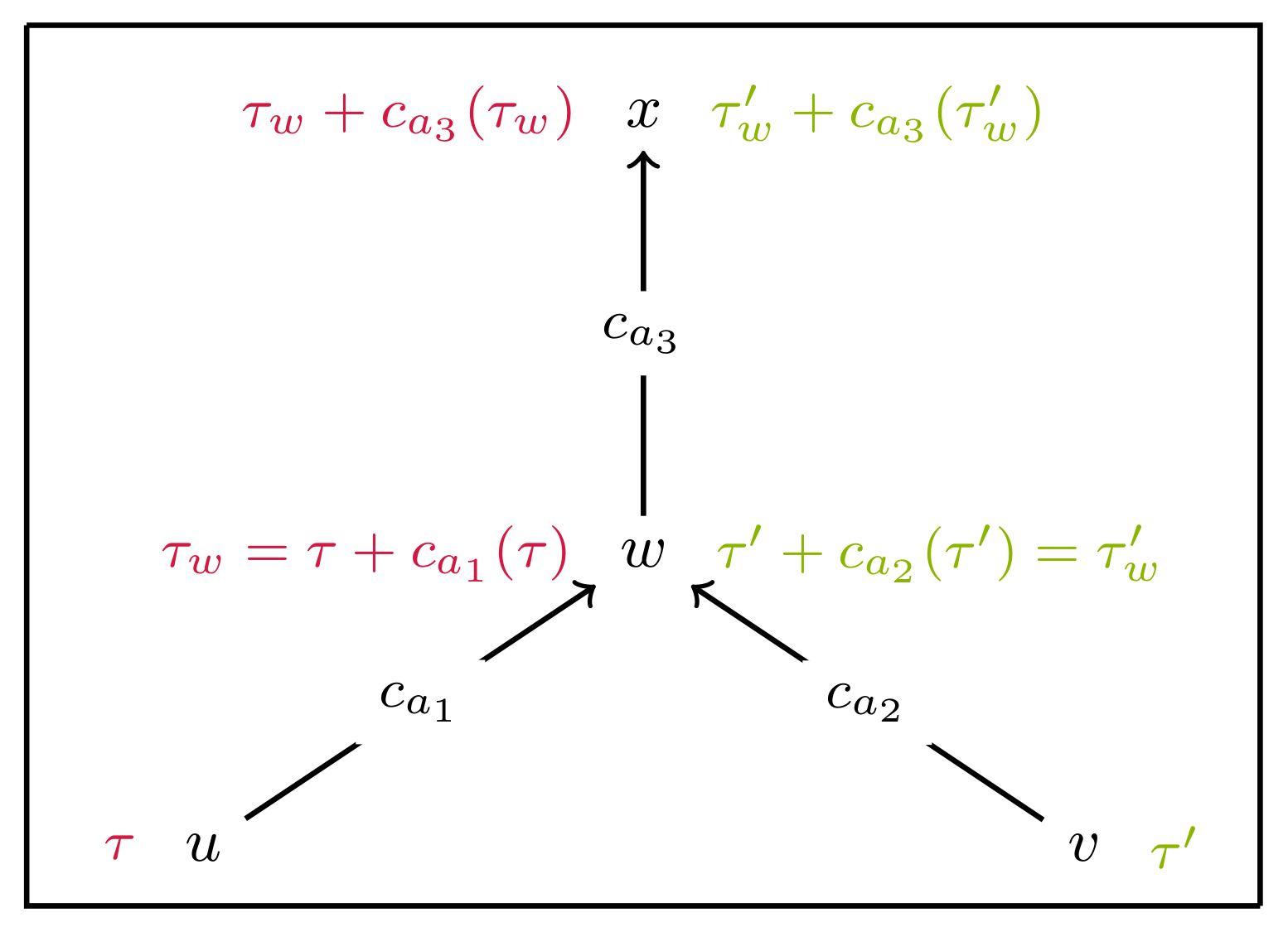
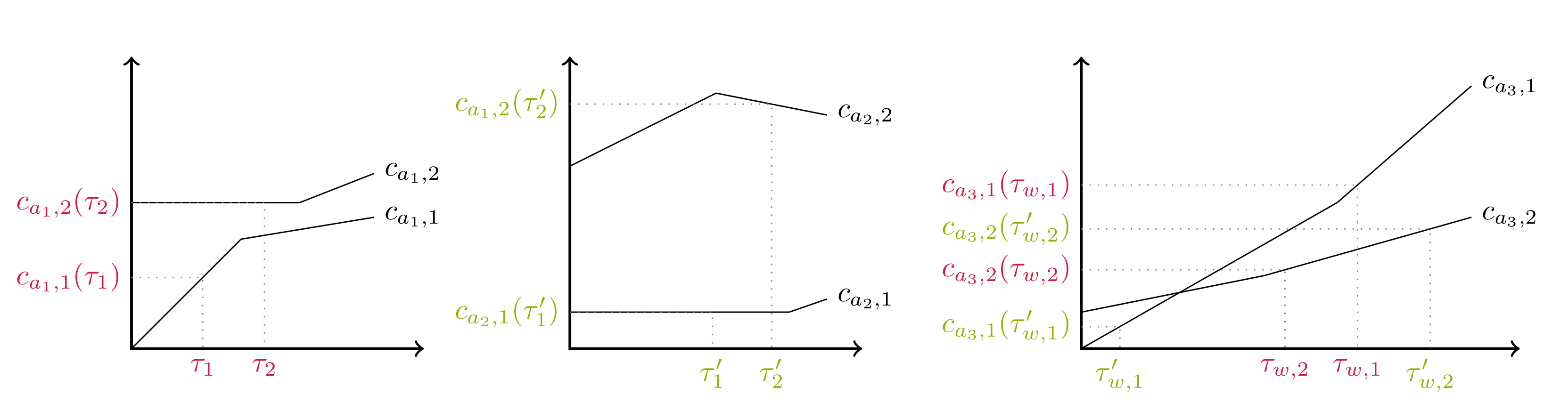
Figure 1 and Figure 2 show an example of a biobjective Dyn-MOSP instance and how the costs of two paths evolve through the corresponding graph. We assume that at the nodes u and v there are paths (red and green) ending with costs and , respectively, and that these paths are now extended towards node x via node w. The plots to the left and in the middle show the costs for traversing the corresponding arc starting with costs τ and , respectively. After the extension along the arcs and both paths meet at node w with costs and . The plots on the right show the arc cost functions corresponding to the arc . Furthermore, on the same diagram, the dominance relationship between both paths at w becomes clear since and . This means that none of the paths ending at w dominates the other one.
3. The Multiobjective Dijkstra Algorithm for Dynamic MOSP Problems
In this section, we discuss Algorithm 1, an adaptation of the Multiobjective Dijkstra Algorithm (MD-A) presented in [16,17] that is extended here to work with dynamic costs. We will see that for the dynamics discussed in this paper, the solvability of MOSP and Dyn-MOSP instances mirrors the well known relationship from the single objective case: if a path p dominates a path at a node v, their extensions inherit this dominance relationship. This characteristic of the cost functions is known as the FIFO property and defined formally in Section 3.2.
3.1. Description of the Algorithm
Whenever we use arrays in our algorithms, we will use an operator to access its elements. To be able to do this on arrays that are indexed according to the nodes or the arcs of G, we assume that these have unique ids from 0 to and from 0 to , respectively. Then, if for example is an array with one entry per arc in G, denotes the content of at the position specified by the id of the arc .
Paths and Labels
In Algorithm 1, paths are considered according to the lexicographically increasing costs. A point is said to be lexicographically smaller than a point () if and only if in the first dimension in which , and we say that a path p is lexicographically smaller than another path if . We will store paths using labels, i.e., by an implicit representation. Let p be an -path (starting at s with costs ) whose last arc is . The label corresponding to p is a tuple , where is a pointer to the label representing the -subpath of p. Note that , which, incurring in an abuse of notation that increases the readability, can be put as . For every node the set contains the labels corresponding to the efficient -paths found during the algorithm. We will see that the label sets will only increase; a label is therefore also called a permanent label. Additionally, a lexicographically sorted priority queue Q stores at most one tentative label per node. Tentative labels correspond to paths that have been explored during the algorithm but are not yet known to be efficient. For a node v, the label stored in Q corresponds to the lexicographically minimal -path that has not yet been made permanent and is not dominated by any label in (we write ).
| Algorithm 1: Multiobjective Dijkstra Algorithm (MD-A) Blue code only for the MD-FPTAS described in Section 4. |
 |
We present the pseudocode of Algorithm 1 in an abstract way, i.e., without specifying the partial order used to define dominance. Instead, we call a function that returns only if a newly found candidate path is dominated by the set of permanent paths at a node, i.e., if this set contains a path that dominates the candidate path. This allows us to use the same pseudocode for the exact algorithm presented in this section and for the MD-FPTAS presented in Section 4. Algorithms 2 and 3 show the function used for the exact MD-A.
| Algorithm 2: for MD algorithm, . |
| 1 return |
| Algorithm 3: for MD algorithm, . |
 |
Iterations
At the beginning, a tentative label is inserted into Q. The main loop of the algorithm retrieves labels from Q; makes them permanent, possibly inserting new labels into Q for the node for which a label was retrieved; propagates their costs, possibly inserting new labels into Q for the successors of this node, and ends once Q becomes empty. Iterations start with the extraction of the lexicographically minimal label from Q, which is added to the end of since it is guaranteed to correspond to an efficient path. Since this is the only way labels are added to the lists , these sets are also sorted in lexicographically increasing order. The main trick in the algorithm is that the queue Q stores at any time at most one label for any node, namely, a lexicographically minimal one that is not dominated by any permanent label at the corresponding node. This makes the algorithm efficient by eliminating any search for non-dominated labels in Q–a tedious task that so far was common to all label setting MOSP algorithms in the literature.
After making permanent, each iteration pursues two main tasks. The first task is to find a new tentative label for v. This is necessary since the priority queue Q stores at most one label for node v at any time. If such a label exists,
is not dominated by any label in and is lexicographically minimal among the labels gained from the extension of labels in , , along the arc (see nextCandidateLabel). This label has to be built every time a label for v is extracted from Q; this is the price for storing at most one label per node. However, it is not necessary to traverse the entirety of the lists every time. Instead, labels in whose extension along were already dominated at the last time a new label for v was built, do not have to be considered. To take advantage of this observation, we store the indices for any arc . These refer to the last checked position in when looking for a label for v and define where a search for v’s next candidate label has to start. If a new label for v is found, it is added to Q. The second task in each iteration is the propagation of along the outgoing arcs of v. The algorithm builds the labels for every and adds them to Q only if . If is lexicographically smaller than w’s current label in Q, the latter is replaced by . In case there is no label for w in Q, is just inserted into Q (see propagate).
| Procedure nextCandidateLabel Blue lines only for the MD-FPTAS described in Section 4. |
 |
| Procedure propagate Blue lines only for the MD-FPTAS described in Section 4. |
 |
Example 2.
Going back to the example shown in Figure 2, assume that the labels ℓ with costs τ at u and with costs at v are in the queue Q and . Then, ℓ is extracted earlier from Q and in the same iteration, Procedure propagate is called to extend ℓ along the arc and obtain the tentative label . We assume that no label for w exists, neither in Q nor in , and hence, is added to Q. Suppose that in the next iteration of Algorithm 1, the label with costs at v is extracted. During its extension towards w in propagate, the label is created. As we can see in the rightmost plot in Figure 2, and hence, . Since the conditions in Lines 3 and 6 of propagate are fulfilled, the label is replaced by , which becomes the new label for w in Q. This however does not discard ! Some iterations later, is extracted from Q and in the same iteration, nextCandidateLabel is called to build a new tentative label for w in Q out of the permanent labels of the predecessor nodes of w. It is in this search where is found again and since it is not dominated (Line 8 of nextCandidateLabel) by any permanent label at w (currently only contains ), it is added to Q. Indeed, as shown in the rightmost plot in Figure 2, and meaning that both labels have to be added to . Later, the label with costs is extracted from Q and finally made permanent. The extension of both labels towards x along works in the same way.
3.2. Correctness
As noted in the beginning of the section, we require the arc cost functions , to fulfill the FIFO property:
Definition 3
(First-In-First-Out Property). The cost function of an arc fulfills the FIFO property if and only if for two cost components , with , there holds .
The correctness of Algorithm 1 relies on the Bellman-Principle [22] of optimality. In the context of MOSP problems, it states that an efficient -path contains only efficient subpaths. Given that the arc cost functions are FIFO, Bellman’s principle holds for efficient paths of the Dyn-MOSP problem. In particular, the following statement holds.
Lemma 1.
Given a Dyn-MOSP instance with FIFO arc cost functions, consider two -paths such that . Then, for the extensions of p and along a -path q in G there holds .
Proof.
Since , we know that for any . Due to the FIFO property of the arc cost functions, this implies that after q’s first arc, say , there holds
This argument can be repeated along every arc of q until we reach the paths’ end point, implying that . □
The consequence of Lemma 1 is that during Algorithm 1, dominated labels/paths can be neglected since they will not become efficient later on. Hence, for a Dyn-MOSP instance whose arc cost function has the FIFO property in every dimension, Algorithm 1 computes a minimal complete set of efficient paths. The rest of the correctness proof proceeds along standard lines as in the static case (cf. [16,17]).
3.3. Complexity
The running time of Algorithm 1 is dominated by the running time of nextCandidateLabel and propagate, that both depend on the complexity of the oracle . It implements the dominance checks that are applied in the different versions of the MD-A that we discuss throughout the paper. In the exact biobjective algorithm, the dominance check (see Algorithm 2) can be implemented in constant time. The reason is that the sets are sorted in lexicographically increasing order and contain only efficient labels. Indeed, the first cost component is sorted in increasing order, while the second cost component is sorted in decreasing order. Thus, a new tentative label that is lexicographically greater than all elements of must only be compared with the last element. This observation seems to be not very widespread in the literature, but given the possibly exponential number of efficient paths at any node, the possibility of checking dominance in constant time has a big impact in theory and practice (cf. [16,17,23]). For the complexity is linear in the number of labels contained in , since in the worst case, the tentative label has to be compared with all existing ones (see Algorithm 3). In our analysis, we will denote the complexity of the dominance check, i.e., of the function , by . We assume that Q is a Fibonacci–Heap [24] to get constant time complexity for the update and the insertion of labels. The label extraction is performed in , since the size of Q is at most n. We set to be the maximal number of labels at a single node at the end of the algorithm. is the total number of computed efficient labels.
Remark 1.
Note that we assume that the evaluation of the arc cost functions can be done in constant time. This is for example the case, when the functions are piecewise linear/constant and the breakpoints are distributed equidistantly. This assumption is common in the literature on Time-Dependent Shortest Paths problems. However, note that logarithmic running times have to be assumed if the breakpoints are spaced without regularity (binary search to find the neighboring breakpoints), or even worse complexities if the functions cannot be easily parametrized. Additionally, we assume that the dimension d of the problem is a constant.
Complexity of nextCandidateLabel
For a node nextCandidateLabel is called every time a label for v is made permanent, i.e., times. The use of the pointers for every arc guarantees that the list of permanent labels at each predecessor node u of v is traversed exactly once. During each call, a dominance check between the extension along of the considered predecessor labels and is performed. This results in a running time of
which summing over all nodes , can be put as .
Complexity of propagate
In total, labels are propagated along an arc . Every time a label is propagated from u along , we have to check if the resulting label is dominated by any label in . Summing over all nodes, we get an overall complexity of
Note that since Q contains at most one label per node, we can have constant time access (e.g., via a pointer) to a node’s heap label. We make use of it in Lines 4 and 6 of propagate.
Algorithm 1 performs one iteration per permanent label, i.e., iterations in total. In addition to nextCandidateLabel and propagate, a label is extracted in every iteration. All in all, the running time of Algorithm 1 is
In Table 1, we list the complexity of the dominance check for the different variants of the MD-A that we consider during the paper. It is clear that the space consumption of Algorithm 1 is if we assume that d is fixed. More in depth discussions of these running time bounds for the exact versions of Algorithm 1 can be found in [16,17].
4. A New FPTAS for the Multiobjective Shortest Path Problem
In this section, we introduce the MD-FPTAS, a new FPTAS for MOSP problems. Basically the MD-FPTAS is Algorithm 1 with a new partial order on the cost vectors, i.e., with a new notion of efficiency. As used for the first time in [2], the main idea is to divide the outcome space into a polynomial number of cells, each of them holding at most one path. The correspondence of a path to a cell is defined via the path’s cost vector. For ease of exposition, we will focus on the static version first. In Section 4.1, we show that the FPTAS also works on Dyn-MOSP instances if some extra assumptions are made about the arc cost functions.
Consider an and two -paths . Then, p-covers q if for all . Let be the set of all feasible paths of a (Dyn-)MOSP instance. A subset is an -cover of if and only if for any there is a that -covers x. If we denote the all-ones vector (initially in d dimensions) by 1, a Fully Polynomial Time Approximation Scheme (FPTAS) for the (Dyn)-MOSP problem is a family of algorithms that computes, for any , a -cover of . Furthermore, its space requirements and running time are polynomial in the size of the used instance as well as in (note that we could define as a vector and get different approximation ratios for every component. However, this would not give deeper insights into the used techniques and is also not used in the experiments presented in Section 5). Additionally, we assume that such that and set , , and for .
As in the FPTAS presented in [2,3], ours is exact in one dimension. In our case, we choose the first cost component to be exact meaning that we compute a -cover of , with . The MD-FPTAS assigns a -dimensional tensor to each node . The entries of each tensor in the dimension, , are indexed from 0 to , for an approximation factor . At most, one -path is stored in each entry of . With our choice of r, this guarantees the desired polynomial running time and space consumption.
The bound on the space consumption can be derived from the size of : the length of becomes for any node and such that, in total, stores at most , a term that is polynomial in the size of the graph and in . If we allow our FPTAS to only store one (simple) path per entry in the vector, we guarantee the polynomial space consumption of the MD-FPTAS. The position of a -path in is computed using the function which is defined componentwise as
This justifies the size of the tensors since efficient (simple) paths have at most arcs and hence, .
We incorporate the subdivision of the outcome space into Algorithm 1 and, in particular, into the dominance checks made therein. To do so, we consider the blue parts in the pseudocodes from Section 3. In the MD-FPTAS any label ℓ representing a path p additionally stores . For ease of exposition, we will write and from now on. Labels continue to be sorted lexicographically in the priority queue Q but the dominance checks are done using the labels’ pos values: if two distinct labels at a node fulfill and for , we say that ℓ-dominates and write . The new checks are shown in Algorithms 4 and 5. No further modifications w.r.t. Algorithm 1 are needed to obtain the MD-FPTAS from the MD-A. Hence, the MD-FPTAS makes labels permanent after extracting them from the heap. It is guaranteed that at the moment of extraction of a label at a node , there is no label in such that and thus, no two labels with the same values will be stored, i.e., nextCandidateLabel and propagate.
| Algorithm 4: for MD-FPTAS, |
| 1 return |
| Algorithm 5: for MD-FPTAS, |
 |
The following example shows how efficient labels can be rejected by the MD-FPTAS if they are -dominated by permanent labels.
Example 3.
Figure 3 visualizes the situation at the end of each of three subsequent iterations of MD-FPTAS. As in Examples 1 and 2, the illustrated graph is a subgraph of a larger graph with nodes and we set . To illustrate how our FPTAS works, dynamic arc cost functions are not needed. Instead, each arc has static cost components. Labels are represented only by their cost vector; their correspondence to nodes is made clear by their positioning. The example starts with a permanent label with costs at node x and tentative labels for u and v in Q with costs and , respectively.
In the first iteration, the label for u is extracted from Q and no new candidate label for u is found. Then, during the propagation of the label , the resulting label with costs at node w is inserted into Q. In the second iteration, the label with costs is extracted from the heap and no new candidate label for v is found. This label is then propagated to node w, where the resulting tentative label with costs is rejected, as w’s current heap label has costs and is lexicographically smaller. So far, the MD-A and the MD-FPTAS would have done exactly the same. In the third iteration, the label with costs at node w is extracted from the heap. When nextCandidateLabel is called, the extension of v’s permanent label towards w yields costs . Hence, it would not be dominated by the new permanent label with costs at w in the exact scenario. However, in the MD-FPTAS, it is rejected since and . The iteration continues and considers the tentative label with costs at node x. It is also rejected despite it would be made permanent in the exact scenario, since and .
The following Lemma holds for any version of Algorithm 1 presented so far. We need it to prove the correctness of the MD-FPTAS. We denote the set of permanent labels at node v found until iteration (including the iteration) by . Thus, is used only to denote the final set of permanent labels at v.
Lemma 2.
A label for a node is considered at most times before it is made permanent or finally discarded. If it is discarded, there is a permanent label in that (pos-)dominates .
Proof.
Let be the permanent predecessor label of at node . is considered for the first time during a call to propagate in the iteration in which is extracted from H and added to . Let be the next iteration wherein a label for node v is extracted from Q. If , we are done since was considered just once before it is made permanent. In case , was either rejected in iteration i because a lex. smaller label for v existed in Q or was replaced in Q by a lex. smaller label for v (Line 7 of propagate) that was not (-)dominated by any permanent label at v. Note that multiple such updates to v’s heap label could have happened until is extracted and made permanent. The iteration proceeds with a call to nextCandidateLabel, where at least one permanent label per predecessor node of v is considered. Since the current iteration is the first time that nextCandidateLabel, is called for v since ’s insertion, points at a label in that is not after . We want to prove an upper bound on the number of times that is considered, so we assume w.l.o.g. that is considered during the current search for v’s new label in Q, i.e., advances at least until ’s position in . Hence, is extended along the arc , generating as a candidate to enter Q in iteration k. According to Line 8 in nextCandidateLabel, is increased if there is a label in that (pos-)dominates . If this happens, later searches for a new tentative label for v no longer consider as a possible predecessor label and hence, ignore . In case , will not be altered and the next search for a new tentative label for v will consider again. Since such searches only happen when a label for v is made permanent, will be considered at most times during calls to nextCandidateLabel. □
The following theorem proves the correctness of the MD-FPTAS for the static case. Its proof is similar to the one given in [3]. Recall that efficient paths can have at most arcs since the arc cost functions are positive.
Theorem 1.
Consider a node and an efficient -path . Then, the MD-FPTAS finds an -path s.t.
Proof.
We prove the statement by induction over k, the number of arcs of . W.l.o.g. we assume that no parallel arcs exist in G. In the base case, we consider an efficient single-arc path . In the first iteration of Algorithm 1, the label corresponding to will be added to Q during propagate. Consider the first iteration in which a label ℓ for node v is extracted from Q. If , we are done since itself is made permanent. In case , Lemma 2 implies that will be made permanent later or be discarded. If it is discarded, Algorithms 4 and 5 guarantee the existence of a permanent label corresponding to an -path such that
and
For , we can derive from (6b) and this in turn can be restated as , which, coupled with (6a), proves the statement. In the induction hypothesis, we assume that
holds for any and efficient paths with arcs.
Induction Step: Let be an efficient -path with k arcs and let be its last arc. Due to subpath efficiency, the -subpath of is efficient. In addition, the induction hypothesis guarantees the existence of a path with corresponding permanent label such that (7) holds for and . When is extracted and made permanent, the label is analyzed in propagate. For the -path corresponding to , we have
From the proof of the base case and from Lemma 2, we know that is going to either be made permanent in a later iteration or be discarded. In case is made permanent, we have and we are done. If is discarded, there exists a permanent label corresponding to an -path p such that and . The latter inequality implies for and, for , is trivially given. Combining this with Euqation (8), we get
which finishes the proof. □
4.1. FPTAS for Dyn-MOSP Problems
From now on we restrict the set of arc cost functions in Dyn-MOSP instances to contain only continuous, piecewise linear FIFO functions. In this case, the proof of Theorem 1 works if the intercepts of the affine functions describing the pieces of the arc cost functions are non-negative. Note that in the proof of Theorem 1 we needed the arc cost vectors only in Equation (8).
Using the notation for dynamic cost, what needs to hold is
To prove the following Lemma, we consider a function with breakpoints and describe the affine functions that build the pieces of f by , .
Lemma 3.
Let be a piecewise affine function with breakpoints and a constant. Then, for points with there holds if the intercepts of the affine functions building f are non-negative for all .
Proof.
We consider three different cases to prove the statement.
Case 1: . Since , we have . Together with this proves the statement.
Case 2: and . In this case, the FIFO property and can be used to get:
Case 3: and . Let be the affine function with and the one with . There holds and we define , , to be the affine function corresponding to the steepest piece of f between y and x, i.e., the one with the biggest . This choice implies and . Additionally, as for any affine function with positive intercept we have . All in all, we can conclude
Together with this proves the statement. □
Now we set , , , and to get that Equation (9) holds under the given assumptions. This enables us to formulate our main Theorem:
Theorem 2
(FPTAS for Dyn-MOSP problems). Let be a Dyn-MOSP instance with continuous piecewise linear and positive arc cost functions that fulfill the FIFO property. Additionally, for any arc let the functions , have only non-negative intercepts. Then, the MD-FPTAS computes a -cover of the minimum complete set of efficient paths for computed by the MD-A.
4.2. Complexity of the MD-FPTAS
In this section, we set . Then, each tensor can store at most paths and when analyzing the MD-FPTAS in terms of and as in Section 3, we get
Recall that the lists contain permanent labels that are sorted in lexicographically increasing order. In the biobjective case this implies that they will be sorted increasingly according to the first cost component and simultaneously, decreasingly w.r.t. their value (Note that for , maps to so it is well defined to talk about a label’s value). There are two reasons for this. On one hand we have the monotonicity of the function and on the other hand, the already discussed fact that for efficient labels that are sorted lexicographically have an increasing second cost component. Hence, as in the exact case, the complexity of the -dominance checks (Algorithms 4 and 5) is constant in the biobjective case and linear () for . Table 2 shows the time complexity of the different FPTAS for the MOSP problem that we are discussing in this paper.
4.2.1. Storing Tensors Explicitly
While the complexity of the MD-FPTAS is lower than that of the Martins-FPTAS, the FPTAS presented in [2] (TZ-FPTAS) is yet to be undercut. This algorithm works similar to the well known Bellman Ford algorithm for the One-to-All Shortest Path Problem and stores the tensor for every node . In iteration , the algorithm computes -paths with at most i edges and does no proper dominance check. Instead, for a newly found path p, the entry in is checked: if it is empty, p is added; if a path already exists, only the one with the lowest costs in the exact dimension (in [2] it is the one) is kept. Since the dominance checks are costly, storing the tensors and checking only the current position yields a great advantage when it comes to the algorithmic complexity.
We can adapt the MD-FPTAS such that at every node a tensor is stored. The entries of are 0 or 1 depending on whether a path with the corresponding value has already been stored in . Let be a tentative label for a node v computed in Line 6 of nextCandidateLabel or in Line 2 of propagate. Instead of calling the function , we check if . In case the tensor entry is indeed set to 0, we add to and set . If the tensor entry is set to 1, we neglect since there is a lex. smaller label in with the same than , hence -dominating .
The suggested adaption increases the space complexity of the MD-FPTAS. Moreover, in general, it will compute more labels than before since checking dominance using is more restrictive than checking -equality. However, as in the TZ-FPTAS, the construction of the tensors still guarantees that the number of paths and iterations stays polynomially bounded. As a consequence, the running time of this variant of the MD-FPTAS for objectives becomes
As shown in Table 2, this is the best known running time bound for an FPTAS for MOSP problems.
5. Computational Results
In this section we provide evince the computational efficiency of the MD-FPTAS in comparison to Martins-FPTAS as presented in [3]; the latter turned out to be faster than the TZ-FPTAS of [2]. Martins-FPTAS is based on the classical label setting algorithm for the MOSP problem by Martins [15]. The data structures are similar to those of the MD-FPTAS. Instead of having at most one label per node in the priority queue, it stores all tentative labels therein until they are extracted or deleted because a label entering the queue dominates them. This iteration through the queue to possibly delete labels is more costly than the searches for a node’s next candidate label performed in the MD-FPTAS. Table 2 shows the complexity of Martins-FPTAS.
5.1. Test Instances
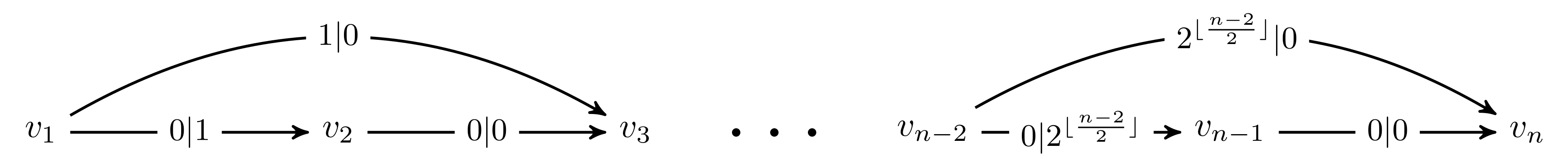
We perform experiments considering 2 and 3 objective functions. In the biobjective static case we use the same instances that were used in [3]. The first group of such instances consists of graphs that contain only efficient paths. These graphs were first described in [1] and are suitable to check the impact of the used approximation techniques (see Figure 4).
We call these instances ; the corresponding graphs have 3 to 51 nodes. The second group of instances, denoted by , are 33 undirected grid graphs of varying size. All instances within have a number of nodes that varies between 1202 and 40,002 and a number of arcs that varies between 4720 and 159,600. The search starts at an artificial node connected to all nodes in the first column of the grid. The costs on the arcs are generated randomly between 0 and 10. The third group of instances are 15 so called NetMaker graphs. They have 3000 nodes and between 30,000 and 80,000 arcs. The source node is always the node with id 0. Both the and instances were first used in [25].
In the 3-dimensional case, we consider a subset of the instances used in [17]. The first set of instances are again NetMaker graphs with an extra cost component. These instances have 5000 to 15,000 nodes and 40,045 to 344,189 arcs. In total, we consider 35 such graphs. Again, the source node is always the one with id 0. We also consider grids with 3 objectives. The undirected grid graph remains unchanged among all instances; we consider 10 different 3-dimensional arc cost functions. These instances are the only ones for which we consider a One-to-One scenario. Trying to solve the One-to-All MOSP problem on these grids was not possible without violating the time limit. Hence, we added the pruning techniques for One-to-One MOSP instances described in [17] to Algorithm 1. It is easy to see that they are compatible with the approximation techniques used in this paper. In total, the instance set contains 300 One-to-One MOSP instances with varying norm between the source and the target node.
The last test instance is a Dyn-MOSP instance motivated by the Horizontal Flight Planning Problem (HFPP) introduced in [26,27]. The directed graph in this instance has nodes and arcs and is called an airway network. The arcs are the direct connections between pre-defined coordinates (the graph’s nodes) along which commercial aircraft are allowed to fly (on www.skyvector.com Sky-Vector an airway network can be displayed). We define two cost functions on each arc. The first one encodes the duration of the traversal of an arc depending on the time point at which the tail of the arc is reached. The duration is influenced by weather conditions and we evaluate the weather information we have every 3h to get 10 data points per arc. The second function models the aircraft is fuel consumption along an arc depending on the aircraft is weight at the arc’s tail node. In our model we get 171 initial weights per arc and the corresponding consumption for each weight. The difference between two consecutive weights is . In both functions, datapoints are interpolated linearly, hence obtaining two continuous piecewise linear functions. The single pieces of the duration function can have positive or negative slopes depending on the wind but the FIFO property still holds as shown in [26]. The consumption function yields an always positive slope since clearly, a higher initial weight will cause a higher consumption. It is therefore also FIFO and, more importantly, the intercepts of its affine pieces are positive, hence fulfilling the requirements from Lemma 3. In total, we have randomly chosen 380 airports as the initial nodes s and compute the ()-efficient paths to all nodes reachable with the full tank of a long-haul aircraft.
5.2. Results
The experiments were ran on a machine with an Intel Xeon CPU E5-2670 v2 @ 2.50 GHz processor. It has two CPUs per node and 10 cores per CPU. The available RAM was . All algorithms were implemented in C and compiled with the version of the GCC compiler with compiler optimization level set at 03. For the priority queues, we used our own implementation of a binary heap. The only difference between the heaps used for the implementations of Martins’s algorithm and those used in the implementations of the MD algorithms is that in the former we took extra care of guaranteeing fast access to a node’s heap labels. This is needed because every time a label for a node v is added to Q, labels for v in Q that are dominated by the new one have to be removed. All lists of permanent labels are modelled as arrays, allowing all algorithms to share the code used for the dominance checks. We set a time limit of for all algorithms. Whenever we report averages, we consider instances that were solved by all algorithms involved in the comparison. The min and max values consider only the results obtained by single algorithms.
5.2.1. Static Biobjective Results
Table 3 summarizes the results of the biobjective MOSP instances. On average, the BDA is 3450 times faster than Martins’s algorithm in the EXP instance set. The average number of permanent labels on these instances is and the maximum is . We computed -covers for the instances with different values for and the average speedup decreases steadily as grows: for , for , and for . This is because , , and of the labels from the exact solution sets are computed for the mentioned values.
Figure 5 gives a visual impression of the running times: on the left hand side we compare the BDA with the FPTAS-BDA and notice how the solution time of the exact algorithm grows exponentially with the number of computed paths. The FPTAS is not faster than the exact algorithms when the number of labels is similar, but on the bigger graphs it saves a lot of labels. On the right hand side we compare the Martins-FPTAS and the BDA-FPTAS. We can see that the running time growth of the BDA is much slower.
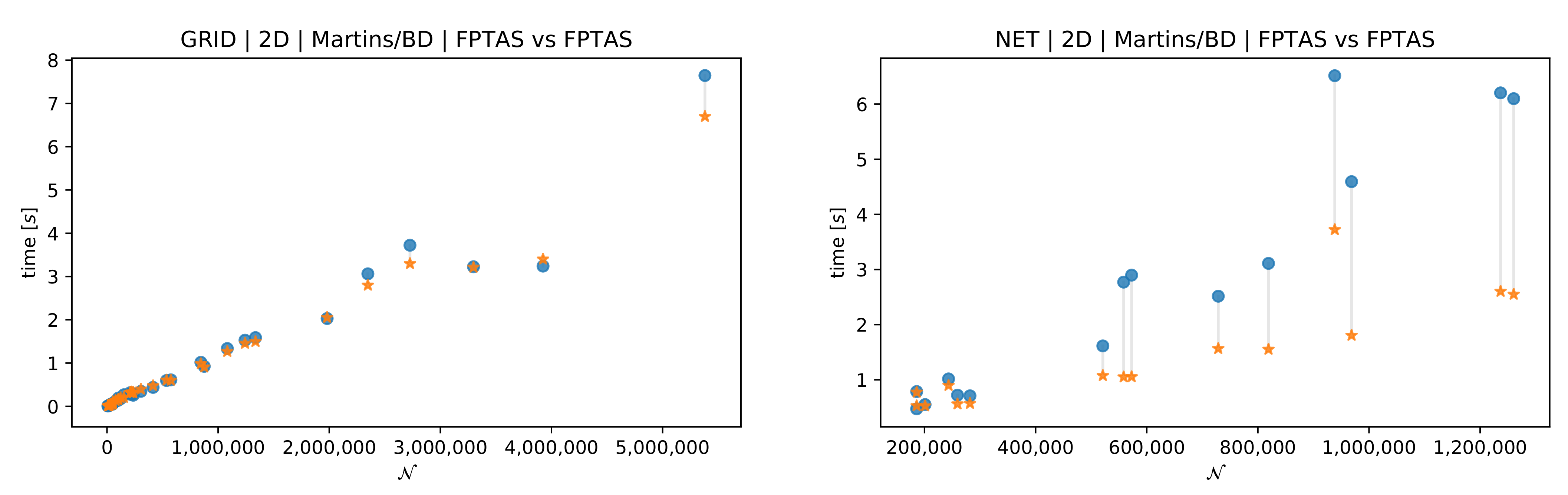
The biobjective and instances unveil the major drawback of the used approximation techniques: on graphs with a realistic/practical amount of nodes, the value of is very close to 1 and the values of any two different paths are almost always distinct. Hence, the exact algorithms are faster than the FPTAS since the computation time of is non negligible in practice and no labels are saved. In [3] the authors overcome this problem by choosing huge values for . Then, they compute an a posteriori approximation that always turns out to be much better than but there is no guarantee for it. Instead, we focus on values for that are consistent with the assumption that we made in Section 4. The consequence is indeed that the average FPTAS speedup for on is and on instances it is , i.e., in both cases a slowdown. On both instance sets the FPTAS solutions contained almost all exact solutions and even increasing up to 1 did not have a noteworthy impact. All algorithms were able to solve all instances in these two sets within the time limit. Figure 6 compares both FPTAS and consolidate the impression gained from the instances: the running time advantage of the MD-FPTAS gets bigger as the number of efficient paths grows.
5.2.2. Static Three Objective Results
Instances with three objectives are much harder to solve. In Table 4, we summarize the results obtained from the One-to-One queries ran on instances and from the One-to-All queries ran on instances. We observe the same behavior as in the instances: a solid running time advantage for the MD-FPTAS on average ( on instances and on instances) for but slower running times than in the exact counterparts. In these experiments all algorithms always computed always the same amount of labels per instance. Figure 7 shows the comparison of both FPTAS’ running times depending on the number of computed paths. In both instance sets the Martins-FPTAS failed to solve bigger instances within the time limit. The overall trend mirrors the biobjective results as the running time of the MD-FPTAS grows considerably slower than that of the Martins-FPTAS.
5.2.3. Our Implementation of Martins’s Algorithm
Note that our implementation of Martins’s (exact) Algorithm and of the Martins-FPTAS is competitive compared to other relevant publications. For example, our biobjective implementation is up to faster than the one used in [3] when solving instances. We believe that the reason is that-as already mentioned-we are using a constant time dominance check in the biobjective case. However, an in depth comparison of the performance of both implementations is not possible: we restricted ourselves to instances that use an approximation factor . This matches the assumption that we made in Section 4 to ensure that .
The direct comparison of our implementation of Martins’s algorithm with the one used in [4] is even harder because the used instances do not coincide. However, the authors try to use vectors whenever possible and use a lexicographically sorted binary heap to store the tentative labels. These choices are similar to ours (we use C arrays) and the reported running times on instances with three cost components are comparable to ours.
5.2.4. Results on Dyn-MOSP Instances
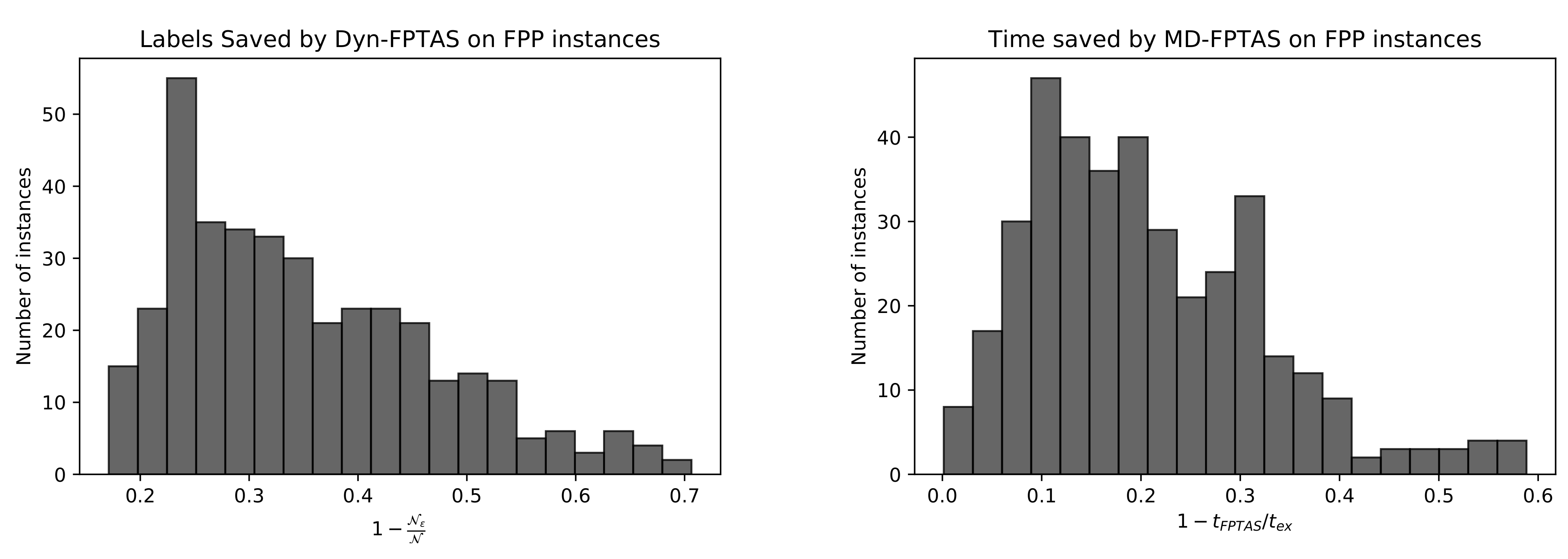
Figure 8 contains histograms showing how the labels (left) and running time (right) savings of the MD-FPTAS are distributed among the 380 considered Dyn-MOSP instances. On average, of the time and of the exact labels can be saved already for .
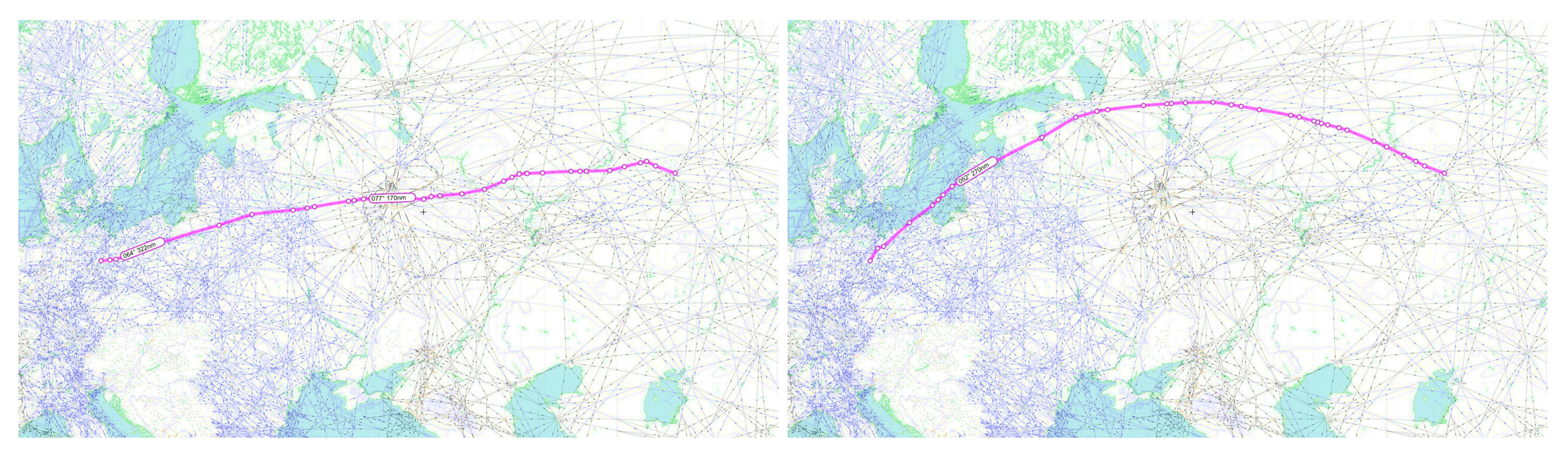
In Table 5, we depicted some geographically distant departure airports and show the impact of the FPTAS when computing routes to all reachable nodes. We finish our computational experiments showing the least consumption and fastest routes from Berlin to Yekaterinburg in Figure 9. Even though consumption and time are correlated objectives, this example shows that both have to be considered since the routes vary considerably.
6. Conclusions
We have proven that Dynamic Multiobjective Shortest Path (Dyn-MOSP) problems can be solved by a generalization of the static Multiobjective Dijkstra Algorithm (MD-A) if the arc cost functions are FIFO and have independent dynamics (e.g., weight and time; time and state of charge). Our main contribution was to adapt the techniques used in the seminal work by Tsaggouris and Zaroliagis [2] to derive a new FPTAS for MOSP problems that is based on the label setting MD-A. The running time of the resulting MD-FPTAS is the number of computed paths multiplied by the running time of the classical Dijkstra algorithm and is thus—to the best of our knowledge—the most efficient FPTAS for MOSP problems in the literature. Even better, it also works for Dyn-MOSP instances if the arc cost functions are FIFO, continuous, and piecewise linear, having only positive intercepts. These requirements are not very restrictive in practice.
We corroborated the theoretical efficiency of our algorithms computationally. On a test set of standard bidimensional and 3-dimensional instances, our MD-FPTAS was faster than the Martins-FPTAS introduced by Breugem et al. [3]. In the static case, we faced the same problem as the authors in [2,3]: the FPTAS does not avoid the computation of paths unless is chosen very large. The reason is that, so far, most instances used in the literature to test MOSP algorithms have integer costs, causing efficient cost vectors to lie at least one cost unit apart from each other. In Dyn-MOSP instances the evaluation of continuous, piecewise linear functions is likely to generate labels with rational cost. This is the case in the Flight Planning instances that we considered. Furthermore, indeed, using realistic values for , we computed -covers for these instances and saved 21% in terms of running time and 35% in terms of labels.
Author Contributions
Conceptualization: P.M.d.l.C., R.B., and A.S.-N.; methodology, P.M.d.l.C., R.B., and A.S.-N.; software, P.M.d.l.C. and L.K.; validation, P.M.d.l.C. and L.K.; formal analysis, P.M.d.l.C., R.B., L.K., and A.S.-N.; investigation, P.M.d.l.C. and L.K.; resources, P.M.d.l.C., R.B., L.K., and A.S.-N.; data curation, P.M.d.l.C. and L.K.; writing—original draft preparation, P.M.d.l.C.; writing—review and editing, P.M.d.l.C., R.B., L.K., and A.S.-N.; visualization, L.K.; supervision, P.M.d.l.C., R.B., and A.S.-N.; project administration, P.M.d.l.C., R.B., and A.S.-N.; funding acquisition, R.B. and A.S.-N. All authors have read and agreed to the published version of the manuscript.
Funding
The researches affiliated to the Zuse Institute Berlin conducted this work within the Research Campus MODAL-Mathematical Optimization and Data Analysis Laboratories-, funded by the German Federal Ministry of Education and Research (BMBF) (fund number 05M20ZBM). Antonio Sedeño-Noda was partially supported by the grant MTM2016-74877-P from the Ministerio de Economía y Competitividad.
Data Availability Statement
Data sharing not applicable.
Acknowledgments
We thank Lufthansa Systems GmbH & Co. KG for providing us with the data used to build our Dyn-MOSP test instances. We also thank Arno Kühner for the helpful and fruitful discussions related proofs and the implementations concerning Dyn-MOSP problems. The authors from [3] provided us with the biobjective Grid and Netmaker instances used in their paper, so we could compare our results with existing data. They got their instances from Andrea Raith, who we also want to thank for providing us with the 3-dimensional instances we used for our computations.
Conflicts of Interest
The authors declare no conflict of interest.
References
- Hansen, P. Bicriterion Path Problems. In Multiple Criteria Decision Making Theory and Application; Fandel, G., Gal, T., Eds.; Springer: Berlin/Heidelberg, Germany, 1980; pp. 109–127. [Google Scholar]
- Tsaggouris, G.; Zaroliagis, C. Multiobjective Optimization: Improved FPTAS for Shortest Paths and Non-linear Objectives with Applications. In Algorithms and Computation; Asano, T., Ed.; Springer: Berlin/Heidelberg, Germany, 2006; pp. 389–398. [Google Scholar]
- Breugem, T.; Dollevoet, T.; van den Heuvel, W. Analysis of FPTASes for the multi-objective shortest path problem. Comput. Oper. Res. 2017, 78, 44–58. [Google Scholar]
- Bökler, F.; Chimani, M. Approximating Multiobjective Shortest Path in Practice. In 2020 Proceedings of the Symposium on Algorithm Engineering and Experiments (ALENEX); Society for Industrial and Applied Mathematics: Philadelphia, PA, USA, 2020; pp. 120–133. [Google Scholar] [CrossRef]
- Emmerich, M.; Deutz, A. A tutorial on multiobjective optimization: Fundamentals and evolutionary methods. Nat. Comput. 2018, 17, 585–609. [Google Scholar] [CrossRef] [PubMed] [Green Version]
- Ehrgott, M.; Gandibleux, X. Multiple Criteria Optimization: State of the Art Annotated Bibliographic Surveys; International Series in Operations Research & Management Science; Springer: New York, NY, USA, 2006. [Google Scholar]
- Ehrgott, M.; Gandibleux, X. A survey and annotated bibliography of multiobjective combinatorial optimization. OR Spektrum 2000, 22, 425–460. [Google Scholar] [CrossRef]
- Ulungu, E.; Teghem, J. Multi-objective shortest path problem: A survey. In Proceedings of the International Workshop on Multicriteria Decision Making: Methods-Algorithms-Applications at Liblice, Czechoslovakia; Glückaufova, D., Loula, D., Cerny, M., Eds.; Institute of Economics, Czechoslovak Academy of Sciences: Prague, Czech Republic, 1991; pp. 176–188. [Google Scholar]
- Current, J.; Marsh, M. Multiobjective transportation network design and routing problems: Taxonomy and annotation. Eur. J. Oper. Res. 1993, 65, 4–19. [Google Scholar] [CrossRef]
- Skriver, A. A classification of Bicriterion Shortest Path (BSP) algorithms. Asia Pac. J. Oper. Res. 2000, 17, 199–212. [Google Scholar]
- Tarapata, Z. Selected multicriteria shortest path problems: An analysis of complexity, models and adaptation of standard algorithms. Int. J. Appl. Math. Comput. Sci. 2007, 17, 269–287. [Google Scholar] [CrossRef] [Green Version]
- Clímaco, J.; Pascoal, M. Multicriteria path and tree problems: Discussion on exact algorithms and applications. Int. Trans. Oper. Res. 2012, 19, 63–98. [Google Scholar] [CrossRef]
- Vincke, P. Problemes multicriteres. Cah. Centre d’ Etudes de Rech. Oper. 1974, 16, 425–439. [Google Scholar]
- Serafini, P. Some considerations about computational complexity for multiobjective combinatorial problems. Recent Adv. Hist. Dev. Vector Optim. 1986, 294, 222–232. [Google Scholar]
- Martins, E.Q.V. On a multicriteria shortest path problem. Eur. J. Oper. Res. 1984, 16, 236–245. [Google Scholar] [CrossRef]
- Sedeño-noda, A.; Colebrook, M. A biobjective Dijkstra algorithm. Eur. J. Oper. Res. 2019, 276, 106–118. [Google Scholar] [CrossRef]
- de las Casas, P.M.; Sedeno-Noda, A.; Borndörfer, R. An Asymptotically and Computationally Improved Multiobjective Shortest Path Algorithm; Technical Report 20–26. ZIB; Takustr: Berlin, Germany, 2020. [Google Scholar]
- Papadimitriou, C.; Yannakakis, M. On the approximability of trade-offs and optimal access of Web sources. In Proceedings of the 41st Annual Symposium on Foundations of Computer Science, Washington, DC, USA, 12–14 November 2000. [Google Scholar] [CrossRef]
- Kostreva, M.M.; Lancaster, L. Multiple Objective Path Optimization for Time Dependent Objective Functions. In Multiple Objective and Goal Programming; Trzaskalik, T., Michnik, J., Eds.; Physica-Verlag HD: Heidelberg, Germany, 2002; pp. 127–142. [Google Scholar]
- Disser, Y.; Müller-Hannemann, M.; Schnee, M. Multi-criteria Shortest Paths in Time-Dependent Train Networks. Exp. Algorithms Lect. Notes Comput. Sci. 2008, 5038, 347–361. [Google Scholar] [CrossRef]
- Foschini, L.; Hershberger, J.; Suri, S. On the Complexity of Time-Dependent Shortest Paths. In Proceedings of the Twenty-Second Annual ACM-SIAM Symposium on Discrete Algorithms; Society for Industrial and Applied Mathematics: Philadelphia, PA, USA, 2011; SODA‘ 11; pp. 327–341. [Google Scholar]
- Bellman, R. The theory of dynamic programming. Bull. Am. Math. Soc. 1954, 60, 503–515. [Google Scholar] [CrossRef] [Green Version]
- Captivo, M.; Clímaco, J.; Figueira, J.; Martins, E.; Santos, J. Solving bicriteria 0-1 knapsack problems using a labeling algorithm. Comput. Oper. Res. 2003, 30, 1865–1886. [Google Scholar] [CrossRef]
- Fredman, M.L.; Tarjan, R.E. Fibonacci heaps and their uses in improved network optimization algorithms. J. ACM 1987, 34, 596–615. [Google Scholar] [CrossRef]
- Raith, A.; Ehrgott, M. A comparison of solution strategies for biobjective shortest path problems. Comput. Oper. Res. 2009, 36, 1299–1331. [Google Scholar] [CrossRef]
- Blanco, M.; Borndörfer, R.; Hoang, N.D.; Kaier, A.; Schienle, A.; Schlechte, T.; Schlobach, S. Solving Time Dependent Shortest Path Problems on Airway Networks Using Super-Optimal Wind. In 16th Workshop on Algorithmic Approaches for Transportation Modelling, Optimization, and Systems (ATMOS 2016); Goerigk, M., Werneck, R., Eds.; OpenAccess Series in Informatics (OASIcs); Schloss Dagstuhl–Leibniz-Zentrum fuer Informatik: Dagstuhl, Germany, 2016; Volume 54, pp. 12:1–12:15. [Google Scholar] [CrossRef]
- Blanco, M.; Borndörfer, R.; Hoàng, N.D.; Kaier, A.; Casas, P.M.; Schlechte, T.; Schlobach, S. Cost Projection Methods for the Shortest Path Problem with Crossing Costs. In 17th Workshop on Algorithmic Approaches for Transportation Modelling, Optimization, and Systems (ATMOS 2017); D’Angelo, G., Dollevoet, T., Eds.; OpenAccess Series in Informatics (OASIcs); Schloss Dagstuhl–Leibniz-Zentrum fuer Informatik: Dagstuhl, Germany, 2017; Volume 59, pp. 15:1–15:14. [Google Scholar] [CrossRef]
Figure 1.
Graph corresponding to the Dyn-MOSP instance discussed in Examples 1 and 2. The corresponding arc cost functions are shown in Figure 2.
Figure 1.
Graph corresponding to the Dyn-MOSP instance discussed in Examples 1 and 2. The corresponding arc cost functions are shown in Figure 2.

Figure 2.
These plots show the two arc cost functions corresponding to the three arcs of the graph in Figure 1: the leftmost functions correspond to the arc ; the functions in the middle to the arc ; the rightmost functions to the arc .
Figure 2.
These plots show the two arc cost functions corresponding to the three arcs of the graph in Figure 1: the leftmost functions correspond to the arc ; the functions in the middle to the arc ; the rightmost functions to the arc .

Figure 3.
Three consecutive iterations of the MD-FPTAS. The extracted label in every iteration is marked in red, the permanent labels in black, and the tentative labels generated in nextCandidateLabel or propagate in grey.
Figure 3.
Three consecutive iterations of the MD-FPTAS. The extracted label in every iteration is marked in red, the permanent labels in black, and the tentative labels generated in nextCandidateLabel or propagate in grey.

Figure 4.
General instance. Every path is efficient.

Figure 5.
BDA exact (green), BD-FPTAS (yellow) and Martins-FPTAS (blue) on exponential instances. .

Figure 6.
BD-FPTAS (yellow) and Martins-FPTAS (blue) on grid instances (left) and netmaker instances (right).
Figure 6.
BD-FPTAS (yellow) and Martins-FPTAS (blue) on grid instances (left) and netmaker instances (right).

Figure 7.
MD-FPTAS (yellow) and Martins-FPTAS (blue) on grid instances (left) and netmaker instances (right).
Figure 7.
MD-FPTAS (yellow) and Martins-FPTAS (blue) on grid instances (left) and netmaker instances (right).

Figure 8.
Distribution of percentage of labels saved by the MD-FPTAS in comparison to the exact MD-A on FPP instances.
Figure 8.
Distribution of percentage of labels saved by the MD-FPTAS in comparison to the exact MD-A on FPP instances.

Figure 9.
Least consumption (left) and fastest (right) routes from Berlin to Yekaterinburg. Source: www.skyvector.com.
Figure 9.
Least consumption (left) and fastest (right) routes from Berlin to Yekaterinburg. Source: www.skyvector.com.


Table 1.
Complexity of the dominance checks.
| Exact MD-A (Section 3.3) | MD-FPTAS (Section 4.2) | MD-FPTAS (Section 4.2.1) | |
|---|---|---|---|
Table 2.
Complexities of the different state of the art FPTAS for MOSP problems. Recall that , and denotes the size of the tensors , i.e., the max. number of paths to be stored at each node.
Table 2.
Complexities of the different state of the art FPTAS for MOSP problems. Recall that , and denotes the size of the tensors , i.e., the max. number of paths to be stored at each node.
| TZ [2] | Martins-FPTAS [3] | MD-FPTAS | MD-FPTAS (Section 4.2.1) | |
|---|---|---|---|---|
Table 3.
Results from one to all runs of biobjective Martins-FPTAS and MD-FPTAS.
| Martins | BDA | |||||||||
|---|---|---|---|---|---|---|---|---|---|---|
| Exact | FPTAS | Exact | FPTAS | |||||||
| 1 | 1 | |||||||||
| EXP | avg | 338,611 | ||||||||
| min | 4 | |||||||||
| max | 1,572,862 | 4213.4131 | ||||||||
| GRID | avg | 872,717 | ||||||||
| min | 8189 | |||||||||
| max | 5,381,078 | |||||||||
| NET | avg | 597,998 | ||||||||
| min | 185,894 | |||||||||
| max | 1,260,412 | |||||||||
Table 4.
Results obtained by 3-dimensional Martins-FPTAS and MD-FPTAS.
| Martins | MDA | |||||||
|---|---|---|---|---|---|---|---|---|
| (o2o)/ (o2a) | Exact | FPTAS | Exact | FPTAS | ||||
| 0.05 | 1 | 0.05 | 1 | |||||
| GRID 3D One-to-One | avg | 8307 | ||||||
| min | 4 | |||||||
| max | 30,041 | |||||||
| NET 3D One-to-All | avg | 13,308,684 | ||||||
| min | 1,170,703 | |||||||
| max | 38,647,047 | |||||||
Table 5.
Running times and computed permanent labels on FPP instances.
| Out-Airport | Exact | |||||
|---|---|---|---|---|---|---|
| Cape Town | 1,537,645 | 917,327 | 817,945 | |||
| Los Angeles | 12,854,272 | 8,260,426 | 7,961,418 | |||
| Moscow | 19,385,407 | 11,458,971 | 10,819,170 | |||
| Berlin-Tegel | 16,815,977 | 12,724,498 | 12,126,247 | |||
| Tenerife | 9,182,417 | 6,247,958 | 5,739,303 | |||
Publisher’s Note: MDPI stays neutral with regard to jurisdictional claims in published maps and institutional affiliations. |
© 2021 by the authors. Licensee MDPI, Basel, Switzerland. This article is an open access article distributed under the terms and conditions of the Creative Commons Attribution (CC BY) license (http://creativecommons.org/licenses/by/4.0/).
Share and Cite
MDPI and ACS Style
Maristany de las Casas, P.; Borndörfer, R.; Kraus, L.; Sedeño-Noda, A. An FPTAS for Dynamic Multiobjective Shortest Path Problems. Algorithms 2021, 14, 43. https://0-doi-org.brum.beds.ac.uk/10.3390/a14020043
AMA Style
Maristany de las Casas P, Borndörfer R, Kraus L, Sedeño-Noda A. An FPTAS for Dynamic Multiobjective Shortest Path Problems. Algorithms. 2021; 14(2):43. https://0-doi-org.brum.beds.ac.uk/10.3390/a14020043
Chicago/Turabian StyleMaristany de las Casas, Pedro, Ralf Borndörfer, Luitgard Kraus, and Antonio Sedeño-Noda. 2021. "An FPTAS for Dynamic Multiobjective Shortest Path Problems" Algorithms 14, no. 2: 43. https://0-doi-org.brum.beds.ac.uk/10.3390/a14020043
Note that from the first issue of 2016, this journal uses article numbers instead of page numbers. See further details here.