Article

Effects of Nonlinearity and Network Architecture on the Performance of Supervised Neural Networks

1
Department of Mathematics, Texas Southern University, 3100 Cleburne Street, Houston, TX 77004, USA
2
Department of Computer Science, Prairie View A & M University, 700 University Drive, Prairie View, TX 77446, USA
3
Department of Physics, Texas Southern University, 3100 Cleburne Street, Houston, TX 77004, USA
*
Author to whom correspondence should be addressed.
Submission received: 20 December 2020 / Revised: 1 February 2021 / Accepted: 1 February 2021 / Published: 5 February 2021
(This article belongs to the Special Issue Supervised and Unsupervised Classification Algorithms)

Abstract

:
The nonlinearity of activation functions used in deep learning models is crucial for the success of predictive models. Several simple nonlinear functions, including Rectified Linear Unit (ReLU) and Leaky-ReLU (L-ReLU) are commonly used in neural networks to impose the nonlinearity. In practice, these functions remarkably enhance the model accuracy. However, there is limited insight into the effects of nonlinearity in neural networks on their performance. Here, we investigate the performance of neural network models as a function of nonlinearity using ReLU and L-ReLU activation functions in the context of different model architectures and data domains. We use entropy as a measurement of the randomness, to quantify the effects of nonlinearity in different architecture shapes on the performance of neural networks. We show that the ReLU nonliearity is a better choice for activation function mostly when the network has sufficient number of parameters. However, we found that the image classification models with transfer learning seem to perform well with L-ReLU in fully connected layers. We show that the entropy of hidden layer outputs in neural networks can fairly represent the fluctuations in information loss as a function of nonlinearity. Furthermore, we investigate the entropy profile of shallow neural networks as a way of representing their hidden layer dynamics.

1. Introduction

The great success of deep learning in applications is based on the clever idea of constructing sufficiently large nonlinear function spaces throughout the composition of layers of linear and simple nonlinear functions (named activation functions). Widely used activation functions include the Sigmoidal function, Rectified Linear Unit (ReLU), and its variants Leaky-ReLU (L-ReLU) and Exponential Linear Unit (ELU) [1,2,3]. Since it was first introduced by Nair et al. [4], ReLU has become one of the most popular choices of activation function for many deep learning applications [5,6]. The ReLU function is defined as ReLU ( x ) = m a x ( 0 , x ) , where x stands for the input. The simplistic ReLU function greatly reduces the computational cost since ReLU ( x ) = 0 when x < 0 . On the other hand, it does cause an information loss in each layer, which could eventually lead to the vanishing gradient problem during the model training [7]. L-ReLU was introduced by Maas et al. [8] to overcome the disadvantage of ReLU and it has the form,
L-ReLU ( x ) = α x , x < 0 x , x 0
where α is the linearity factor ( 0 < α < 1.0 ). Note that the L-ReLU with α = 0 is the ReLU function and it becomes the identity function when α = 1 . In practice, the value of α is kept closer to zero. However, there is no supporting theory to predict the ideal value of α . Instead, it is usually determined through trial-and-error observations. Similarly, selection between ReLU and L-ReLU for a certain network is determined by prior experimental knowledge. Usually, investigation of the information loss due to the use of activation functions is not given a priority since the accuracy is used as the primary method of evaluating the performance of many deep learning models. However, when it comes to shallow networks, effects of activation functions may play an important role in understanding the learning process and for the interpretation of results. Therefore, a study of experimental evidence to enhance our understanding of the behavior of activation functions is necessary in order to minimize the possible speculations. The amount of nonlinearity of a deep network results from the composition of the layers of nonlinear functions. Therefore, the impact of different activation functions on the final performance is likely linked to the model architecture (width and the depth). In addition, as pointed out by D’Souza [9], model performance also depends on the data type (for example, continuous, categorical, calligraphic, or photographic).
Based on the considerations above, we take α as a measure of nonlinearity introduced by an activation function and study the model performance for different choices, and in conjunction to different network shapes and architecture, as illustrated in Figure 1, with examples chosen from a wide range of data domains. We use the entropy, a measurement of randomness or disorder, for the estimation of information flow in shallow neural networks. Entropy, H(x) of a random variable x is defined as,
H ( x ) = i = 1 n P ( x i ) l o g P ( x i )
where, P ( x i ) represents the probability of ith outcome and n represents the total number of distinct outcomes. Entropy can be calculated from the output of each hidden layer of a neural network during the training. When the sample space for the hidden layer output becomes larger, the randomness increases and therefore the entropy increases. If the output of hidden layers become more ordered then the entropy must decrease. Note that the entropy is always a positive quantity. The training process of a neural network can be visualized as going from a random initial function state with larger entropy to a more ordered function state with less entropy. Since the entropy can be calculated per each layer separately, it can be used to track the layer dynamics during the training.

2. Background and Objectives

Researchers have been thoroughly investigating the selection process of activation functions for a given modeling task ever since the deep learning became practical with modern technology. As a result of empirical and theoretical advancements in the field, there are multiple studies that propose the use of new activation functions [4,8] while others discuss the effects and reliability of them in deep networks [10,11,12]. However, ReLU still remains the most popular and effective activation function in many deep learning models [11]. Rectifier activation is first discussed by Hahnloser et al. in 2000 with regard to its biological motivations [13] and later in 2010 it is introduced as ReLU by Nair et al. [4]. In 2011, the successful use of the rectified activation in deep learning for large data sets was demonstrated by Glorot et al. [10]. As a method that applies a variable non-linearity into ReLU, the activation L-ReLU was discussed in parallel to the introduction of ReLU in deep learning [8]. Nwankpa et al., compares the effects of activation functions with the state-of-the-art research results and outline the trends and functionalities such as feature detection capabilities associated with the activation functions [2]. However, there is lack of insight into the effects of activation functions as an important hyper-parameter on the performance of deep learning models.
Optimization of hyper-parameters of neural networks are often analyzed by Auto Machine Learning Tools [14]. Hutter, F., et al. [15] introduced an ANOVA based approach to understand the effects of hyper-parameters in deep learning. Probst, P., et al. [16] and van Rijn, J.N., et al. [17] have presented a study on the importance of hyper-parameters across different data sets and algorithms. They mainly focus on the commonly used algorithms such as, support vector machines, random forests and Adaboost. An interesting work done by Chen, B., et al. [18] describes a method of hyper parameter optimization in neural networks using a network construction algorithm. Lee, A., et al. [19] explore the significance of automated approaches to find best hyper-parameters for machine learning workflows. However, in neural network models, the number of layers (depth) and the number of nodes per layer (width) or in other words, the shape of the architecture has been studied as the most important hyper-parameters [20]. In this study, we show that the correct selection of most commonly used activation functions, ReLU and L-ReLU is as important as the selection of the shape of the network architecture for optimal results.
The ReLU activation only allows to pass positive input and cuts-off the negative inputs. This is shown to be problematic in the training of neural networks and often leads to dying neurons [21]. In practice, possible empirical remedies to overcome this problem is either to lower the learning rate or if possible, to reduce the depth of the network. However, L-ReLU on the other hand becomes a handy alternative to ReLU in such situations which has been discussed extensively by Maas et al. [8]. There are several recent studies done on the information flow and information loss optimizations in neural networks [22,23] in which authors discuss about the information loss due to the limitations in data sampling, and data encoding. It is equally important to address the variations in information flow in neural networks due to the nonlinearity in the network since the application of nonlinearity is an essential tool in deep learning. Furthermore, discussions on the non-linearity in L-ReLU are not widely available in literature compared to the studies based on ReLU. Because of its flexibility, nonlinearity in L-ReLU can be adjusted to affect the information flow and the model accuracy in shallow neural networks, and the effects of nonlinearity in neural network models may depend on the model architecture, feature extraction techniques and the type of input data.
In this study we provide our findings about the effects of nonlinearity in neural networks, using widely used activation functions, ReLU and L-ReLU and give justifications to the observations as an insight to the deep learning process. We empirically show that the ReLU is a reliable activation function when there is sufficient number of trainable parameters in the network. However, in the case of transfer learning, we show that the L-ReLU improves the classification accuracy than ReLU when used in classification layers. In addition to that, we investigate the effects of nonlinearity in L-ReLU for different modeling approaches and data domains. We show that the information loss due to the nonlinear activation can be interpreted using entropy. Finally, we show that the entropy of the hidden layer outputs of a neural network has a connection to its optimization process. The entropy change during the training process helps to visualize the transformation of function space from a disordered to a more ordered sate as the training progresses.

3. Results and Discussion

In the following sub-sections, first we discuss the effects of nonlinearity in the network on the performance of shallow neural networks. We do this using different network architectures shown in Figure 1 and by training them using 20,000 MNIST-digits images [24] and 20,000 MNIST-fashion images [25] with a 33% validation split. Then, we compare the effects of nonlinearity in the presence of different data domains using 60,000 MNIST-digits data, 60,000 MNIST-fashion data, 60,000 EMNIST-letters data [26] and simulated continuous data of same sample size. Next, we address the importance of controlled nonlinearity in the classification layers of neural networks when the transfer learning is used to extract important features (bottleneck features) from image data. Finally, we show the entropy estimation in the hidden layers of shallow neural networks using 60,000 MNIST-digits images and 60,000 MNIST-fashion images with 33% validation split. There, we investigate the variations in the entropy profile of shallow neural networks and its connection to the nonlinearity and to the complexity of the network using different network architectures.
The construction of the deep learning models as well as the model training were done using the deep learning tools (Scikit-learn, TensorFlow-keras and Pytorch) [27,28,29]. Refer to our GitHub repository (GitHub:https://github.com/nalinda05kl/nonlinear_activations, accessed on 20 December 2020) for detailed analysis codes used in this study. The computations were conducted mainly using a computer resources allocation grant from the Pittsburgh Super-Computing Center (PSC) [30].

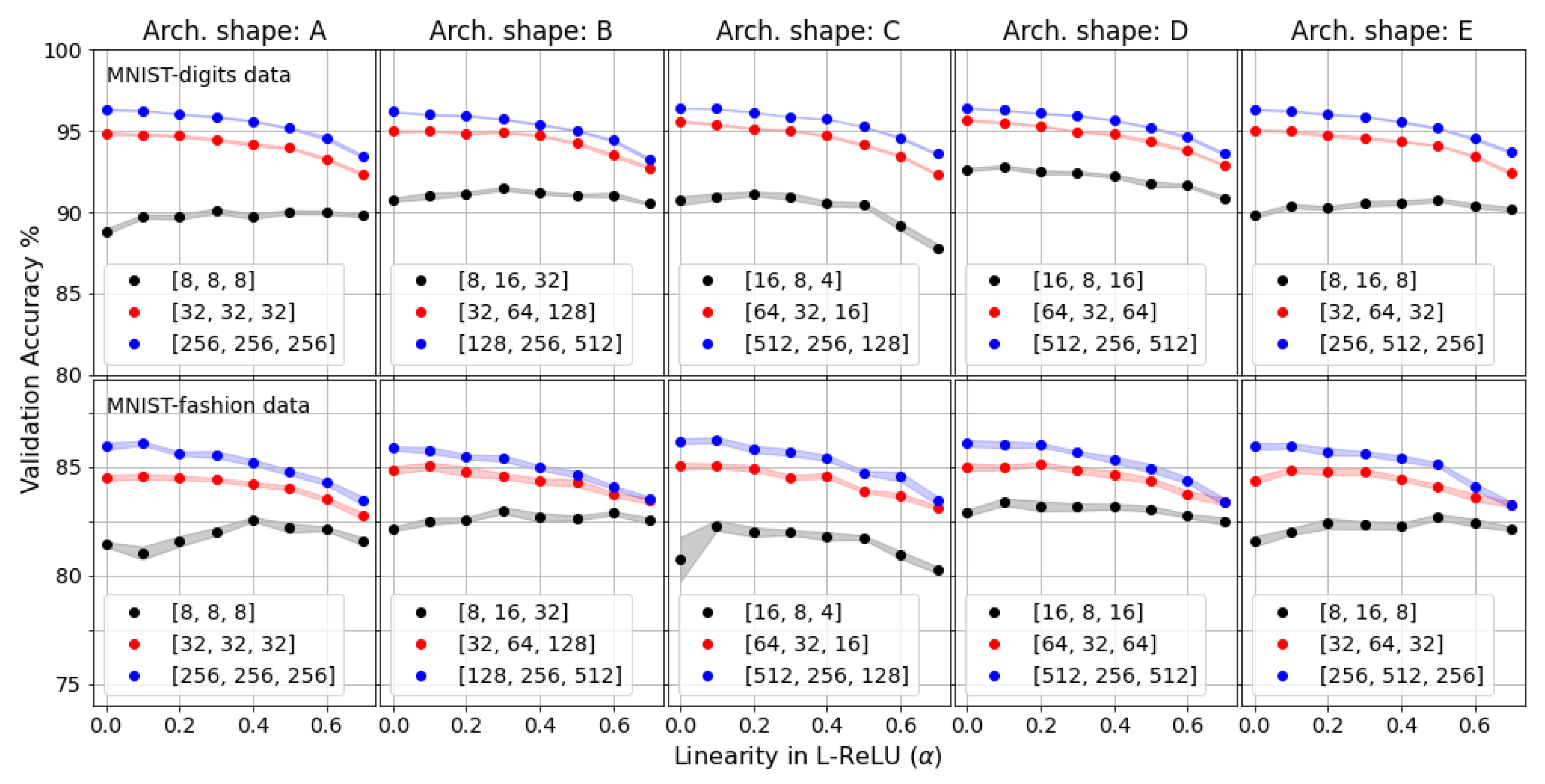
3.1. Effects of Nonlinearity in Different Network Architectures

For this test, we use five model architecture shapes (Figure 1), each with three hidden layers. ReLU or L-ReLU (with variable nonlinearity) were used as the activation function. For the convenience, we will refer to the shapes of the network shown in Figure 1A–E as Architecture A–E. Architecture A consists of a constant number of nodes per hidden layer while in the other four architectures (Architecture B–E) the number of nodes varies from layer to layer. In Architecture B and C, the ratio between the number of nodes in two consecutive layers is constant while in Architecture D and E, the ratio between the nodes in first two layers is the reciprocal of the ratio between the number of nodes in last two layers. The complexity of each model architecture was varied by changing the number of nodes per hidden layer according to the combinations shown in Table 1. We trained the models for total of 20 epochs and present the maximum validation accuracy obtained during the training process. We used stochastic gradient descent [31] with a learning rate of 0.1 as the optimizer, and the categorical cross entropy [32] as the loss function.
We explored the effect of the linearity factor, α on the model performance based on the five architectures illustrated in Figure 1 with different number of trainable parameters. Figure 2 shows the maximum validation accuracy for Architectures A–D as a function of α for MNIST-digits images and MNIST-fashion images with the uncertainties estimated by the standard error. Note that, in the error estimation, we were mainly concerned about the uncertainty arises due to the parameter initialization (initial conditions) of the models. Therefore, the uncertainties were calculated by training the models 20 times with randomized weight initialization in each run and, by taking the standard deviation of results obtained in all runs. As shown in Figure 2, for the Architecture shapes A–D, the model accuracy increases as the number of parameters is increasing for all values of α . One interesting observation in Figure 2 is that, for both MNIST-digits and MNIST-fashion data sets, L-ReLU was able to increase the validation accuracy only when the number of parameters were relatively small (data points in black), regardless of the shape of the model architecture and the data set used for the training. Based on these observations, in Table 2, we show the optimal value for the liniarity factor, α for each model architecture (Arch. A–E) discussed in this study (see Table 1 for the number of nodes used in each model architecture). According to Table 2, it is clear that the optimized value for the linearity factor decreases (approaches zero) as the width of the network increases. That means, for networks with sufficiently large number of trainable parameters, ReLU is a better choice for the activation function. A possible reason for L-ReLU being a better alternative to ReLU for small networks could be that ReLU has suppress some essential information that were preserved by L-ReLU (in a regularized fashion). When the network becomes wider, the increase in the number of trainable parameters enlarges the feature representation space so as to efficiently capture more essential features with ReLU than with L-ReLU.
Next, the effect of the shape of the network architecture on the model performance was tested as a function of linearity factor, α (results are shown in Appendix A.1). Here (in Figure A1a), the number of parameters were kept approximately constant ( 10 5 ± 1%) while changing the shape of the model architecture (from A to E). We observe that there is no effect of the shape of the model architecture on the accuracy for ReLU and for all the values of α in L-ReLU. This observation reveals that the model performance is not highly correlated with the shape of the network architecture in comparison to the correlation of the model performance with the number of parameters. It seems that the most important factor for model accuracy is the number of parameters rather than the shape of the model architecture. However, as seen in Figure A1b number nodes in the first layer must be sufficient to capture the feature space otherwise the model suffer from under-fitting even with larger number of trainable parameters.

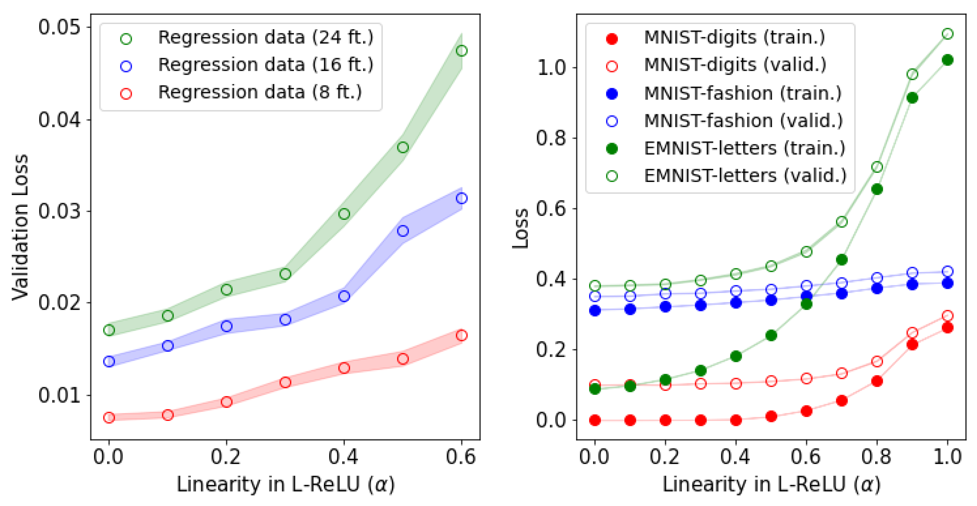
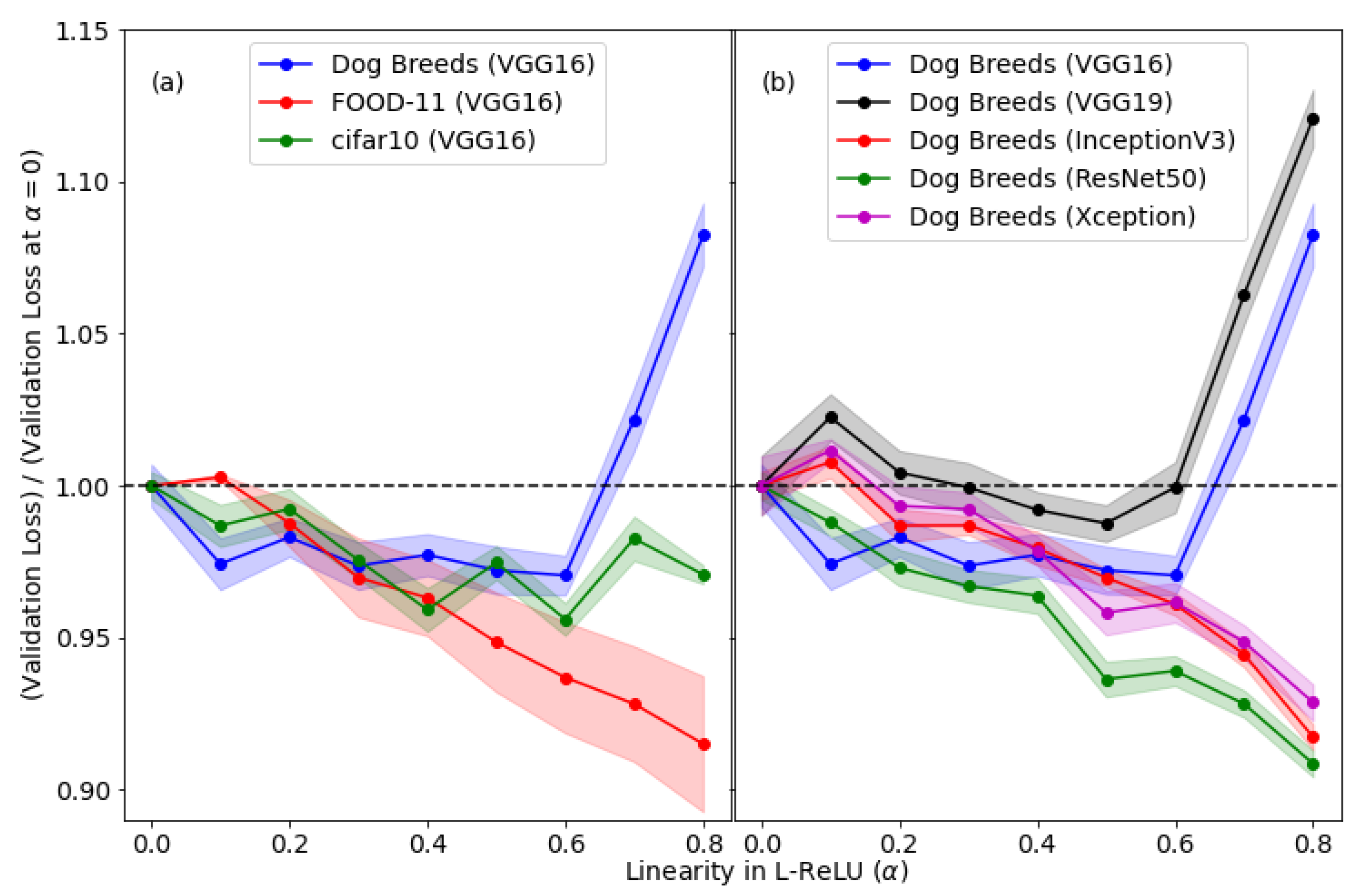
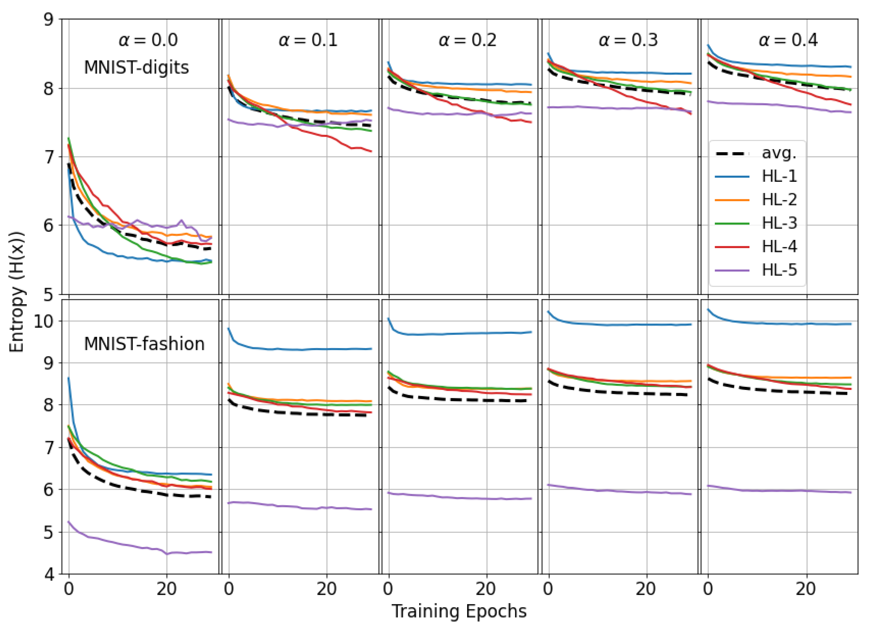
3.2. Effects of Nonlinearity for Different Data Domains

In Figure 3, we show the trends in validation loss as a function of linearity factor, α in L-ReLU using two types of data sets: continuous data (left panel) and categorical image data (right panel) by comparing results form six databases in total. In this test, the shape of the model architecture and the number of nodes in each hidden layer of the fully connected network were set to a fixed sequence as explained in Appendix A.4, Table A2 and Table A3. Three categorical data bases (MNIST-digits data, MNIST-fashion data and EMNIST-letters data) each with 60,000 sample size were used to study and compare the results. To interpret the effects of nonlinearity for continuous data with different dimensions, results are presented for 3 continuous databases with 8, 16, and 24 features, each with 60,000 sample size. Continuous data were simulated according to the following model using a Gaussian noise with standard deviation of one.
f ( x ) = exp ( n = 1 N a n x n ) + Gaussian Noise
According to Figure 3, left panel, for the continuous data, the validation loss increases significantly as a function of α and, we only show the results up to α = 0.6 because, the training loss for the continuous data become unstable and rapidly increases when α is greater than 0.6. Validation loss for regression data with 16 and 24 features reaches an extremely large value at α = 1 (in the order of 10 4 ). This demonstrates the need for ReLU when training data consist of features nonlinearly related to the target variable (see Equation (3)). Furthermore, in Figure 3 left panel, the model with α = 0.6 shows much weaker performance on the data set with 24 features (in green) compared to results obtained using the data set with eight features (in red). This observation shows the inability of L-ReLU in capturing the nonlinear function space when the data becomes complex with more input features.
According to Figure 3, right panel, the dependence of validation loss on α for categorical image data is much weaker compared to the continuous data and it does not blow-up even at α = 1 . This may be due to the nonlinearity in the softmax activation function applied to the last layer of the model. That means, even at α = 1 , the softmax activation in the last layer preserves nonlinearity which prevents the validation loss from blowing up. The ReLU function adds strong nonlinearity to the network in comparison to the L-ReLU and enhances the independent learning in each hidden layer. This could be one possible reason for why the validation loss at α = 0 happens to be the best value for both continuous and categorical data sets. Another interesting observation in Figure 4, right panel is that the dependence of loss on α for EMNIST-letters data is much stronger (green curve) compared to the MNIST-digits and MNIST-fashion data and the model with α = 1.0 shows the worst performance of all. Compared to number of classes in the MNIST-digits and MNIST-fashion data (each has 10 classes), the EMNIST-letters data has more classes (26) and the results suggest that the ReLU becomes most efficient when the number of classes in the database is relatively large.
In Figure 4, we show the validation loss (with respect to the validation loss at α = 0) as a function of α when transfer learning is used to extract important features in image classifications. Transfer learning is very efficient when there is limited number of images available to train a model. Small databases make the model-training quite difficult, specially in image classifications. In such situations, pre-trained models can be used to extract the important features (bottleneck features) from the images. A block with classification layers must be built on top of the pre-trained model and it is trained to classify the bottleneck features extracted from the pre-trained model. This classification block often consists of fully connected layers and uses nonlinear activation functions. However, the use of strong nonlinear functions in the classification layer could destroy the useful information extracted using transfer learning. To investigate on this matter, we have studied the effects of nonlinearity in the classification layers on the model performance when the transfer learning is used.
First, we used three data sets: FOOD-11 [33], cifar10 [34] and Dog Breeds [35] and extracted the bottleneck features using the pre-trained model VGG16 [36] (pre-trained using ImageNet data [37]) and results are shown in Figure 4, left panel. It is clear that the L-ReLU performs better for all three data sets compared to ReLU. However, we observed that, for both cifar10 and Dog Breeds data, classification layers with L-ReLU were not able to fit to data when α = 1 and the increasing trend in validation loss is visible for Dog Breeds data set after α = 0.6 . In Figure 4, right panel, we show the validation loss (with respect to the validation loss at α = 0 ) for Dog Breeds data using five pre-trained models [36,38,39,40]. For all five pre-trained models, we observe that the model performance improves as the α is increased. However, both VGG-16 and VGG-19 models show week performance after α = 0.6 .
Due to the transfer learning, we can assume that, most of the important information is already extracted into the bottleneck layer. In addition, the nonlinearity is already applied to pre-trained models through nonlinear operations such as ReLU activation function and max-pooling operations. Therefore, the use of a strong nonlinear activation function (ReLU) to classify the bottleneck layer does not seem to be improving the accuracy. Instead, there is a loss of important information caused by the application of ReLU in the classification layers.
Above results suggest that the amount of information passed to the next layer by the activation function has a significant effect on the model performance. We find that, it is worth quantifying the level of information flow in the network and analyzing how it is affected by the nonlinearity of activation functions. As a solution for that, in the next section, we use entropy as a quantitative measurement for the information flow in shallow neural networks to better understand the effects of the nonlinearity on their performance. We also show that the entropy can represent the training dynamics in shallow neural networks.

3.3. Entropy Profile of Shallow Neural Networks

In this section we discuss the possibility of using the entropy as a measurement of randomness to represent the information flow in the shallow neural networks. This study is necessary since the use of activation functions and different model architectures affects the information flow in neural networks, which ultimately could affect the performance of the model. We have already shown that the use of different linearity factors affects the model performance in both regression and classification examples that were discussed in this paper.
For this study, entropy estimation was performed for each training epoch, using the output of each hidden layer of a shallow neural network with 5 hidden layers. Output of each hidden layer was divided in to 100 equal sized bins and the resulting distribution was used to calculate the entropy (Equation (2)). Figure 5 shows the entropy calculated in a neural network with five hidden layers while changing the linearity factor from α = 0 to α = 0.4 for two databases: MNIST-digits and MNIST-fashion using 60,000 images from each database with a 33% validation split. The number of nodes in hidden layers 1–5 of the model architecture used for this analysis were 256, 128, 128, 128 and 32, respectively. We used the Negative Log Likelihood Loss (NLLLoss) [41] as the loss function and Adam optimizer [42] for the model optimization.
As seen in Figure 5, for both MNIST-digits and MNIST-fashion data sets, the entropy of each hidden layer in the network increases as the linearity factor ( α ) is increasing. When the value of α is increased, the negative values are allowed to flow through the network. Therefore, the randomness in the hidden layer outputs becomes enhanced due to the increase in the number of possible outcomes when compared to the α = 0 situation. This observation suggest that the entropy can be used as a measure of randomness in hidden layer outputs to visualize and quantify the information flow in neural networks. In addition to this observation, we can also see that the entropy of most layers decrease as the training progresses. This is due to the decrease in randomness of hidden layer outputs as a result of parameter optimization. Since the network is initialized with random parameters, the output of each hidden layer is expected to be highly random leading to a relatively higher entropy at the beginning of the training. However, as the training progresses, the model converges into a state where the composition function represented by the neural network has hidden layer outputs that are more ordered and stabilized leading to a lower entropy. In practice we use the learning curves as a evaluation of the learning process of the whole network together. In conjunction with the learning curve, the entropy profile leads to a better understanding of the overall dynamics of the neural network, as well as detailed analysis from a layer-by-layer perspective.
As the next step, we further investigate the entropy profile of shallow neural networks to track the learning process during the model optimization as a function of model complexity. Results are shown in Figure 6 and Figure 7 for different model architectures trained using 60,000 MNIST-digits data (we also have used 60,000 MNIST-fashion data and obtained similar results for the entropy profile as shown in Appendix A.2 and Appendix A.3). The activation function used in these models is the L-ReLU with α = 0.1 . The complexity of the model is changed by increasing the number of hidden layers from two to five (note that the number of nodes per hidden layer is kept fixed in Figure 6). In Figure 6, the validation loss reaches its minimum value at different epochs for different models. However, the model with two hidden layers shows the weakest performance since its minimum validation loss is the worst of all models tested. Interestingly, the corresponding average entropy of this network is relatively greater when compared to the other networks.
We further tested the entropy profile of shallow neural networks as shown in Figure 7. Here, the shape of the network architecture we used is different than what is used in Figure 6, where the number of nodes per hidden layer is changed as shown in Figure 7, lower panel. On the contrary to the observations we have seen in Figure 6, here we do not see higher average entropy for the networks with weak performance. Instead, the average entropy for all network architectures show similar values regardless of their performance. Therefore, we do not observe a direct relationship between entropy and the model performance. However, the variations of entropy in individual layers must be studied thoroughly since the entropy of some layers (such as, hidden layer one and two of 5-hidden layer network in Figure 7) increases after few epochs of training time. In most cases this effect arises when there is relatively a small number of nodes present in a certain layer. Such a layer can be visualized as a histogram with few bins (less than needed) to represent the data. In such situations, shape of the output distribution could be suppressed and becomes more random. As a result, the entropy can become enhanced. Other than that, we do not see a connection of the increasing entropy in those layers to known complications in the training process such as the over-fitting or under-fitting. However, the increase in entropy in some layers visualizes the effects of suppressed information.
There are several limitations and possible validations for this study that may be addressed as future directions. There are several Auto-ML packages [14] that can be used in hyper-parameter optimization. A compassion of the results we discuss in this work with the results from Auto-ML tools could become useful for further validation of the observations we have. Although, the entropy was able to reflect the information distribution through the randomness in hidden layer outputs, other established measurements like the Kullback–Leibler Divergence (KL-Divergence) [43,44] which is also known as the Information Gain would show a similar picture of the information flow during the learning process. However, it is a challenge to calculate KL-divergence using discrete hidden layer outputs, specially in the case of image data, unless a function approximation is used to represent the output distributions.

4. Conclusions

We have extensively analysed the effects of the number of parameters, shape of the model architecture and nonlinearity on the performance of deep learning models. We found that the L-ReLU function is more effective than ReLU only when the number of parameters is relatively small, according to the tests conducted using MNIST data using shallow neural networks (all observations are summarized in Table 2). We show that, for shallow neural networks, the shape of the model architecture is less important compared to the number of trainable parameters, for the enhancement of the model performance, regardless of the nonlinearity in the network. Then, we looked into different data domains (continuous, categorical with or without transfer learning) as inputs to the networks and their effects on the model performance under different nonlinearities in the network. Results show that, for classification and regression examples that do not use transfer learning, strong nonlinearity (values of α closer to zero) increases the performance of the model. However, in the case of using transfer learning to extract bottleneck features, we found that the use of L-ReLU in the final fully connected layers shows better accuracy than the use of a strong nonlinear function like ReLU. Finally we introduced the entropy as a way of quantifying the information flow in shallow neural networks. We observe that the average entropy of shallow neural networks increases as the nonlinearity of the network is decreased. Therefore, we suggest the entropy as a way of quantifying the information loss due to the use of nonlinear activation functions specially for shallow neural networks. Furthermore, we show that the entropy evolution of the hidden layer outputs can fairly represent the transformation of composition function space from a disordered initial state to an ordered final state during the training. However, we do not observe strong evidence linking the model performance to the variations in the entropy profile of neural networks.

Author Contributions

Conceptualization, Y.W. and D.V.; methodology, N.K.; validation, N.K. and N.R.R.; initial numerical study, Z.K.; formal analysis, N.K.; writing–original draft preparation, N.K. and Y.W.; writing–review and editing, Y.W., D.V. and N.R.R.; visualization, N.K.; supervision, L.H., D.V. and Y.W.; funding acquisition, Y.W., D.V. and L.H. All authors have read and agreed to the published version of the manuscript.

Funding

This work is funded by the National Science Foundation (NSF), grant no: CNS-1831980, CNS-1832034, PHY-1831977, and HRD-1800406. Initial computational work in this study was conducted using computational resources at high performance computing centers at Texas Southern University and Prairie View A&M University. This work used the Extreme Science and Engineering Discovery Environment (XSEDE), which is supported by National Science Foundation grant number ACI-1548562. Specifically, it used the Bridges system, which is supported by NSF award number ACI-1445606, at the Pittsburgh Supercomputing Center (PSC).

Institutional Review Board Statement

Not applicable.

Informed Consent Statement

Not applicable.

Data Availability Statement

Publicly available data sets were analyzed in this study.
This data can be found here:
(a). MNIST-digits (http://yann.lecun.com/exdb/mnist, accessed on 20 December 2020),
(b). MNIST-fashion (https://github.com/zalandoresearch/fashion-mnist, accessed on 20 December 2020),
(c). EMNIST-letters (https://www.kaggle.com/crawford/emnist, accessed on 20 December 2020),
(d). cifar10 (https://www.cs.toronto.edu/~kriz/cifar.html, accessed on 20 December 2020),
(e). FOOD-11 (https://www.kaggle.com/vermaavi/food11, accessed on 20 December 2020),
(f). Dog Breeds (http://faceserv.cs.columbia.edu/DogData, accessed on 20 December 2020).

Acknowledgments

Authors thank Alice Xu for her contribution in language editing and proof reading.

Conflicts of Interest

The authors declare no conflict of interest.

Appendix A

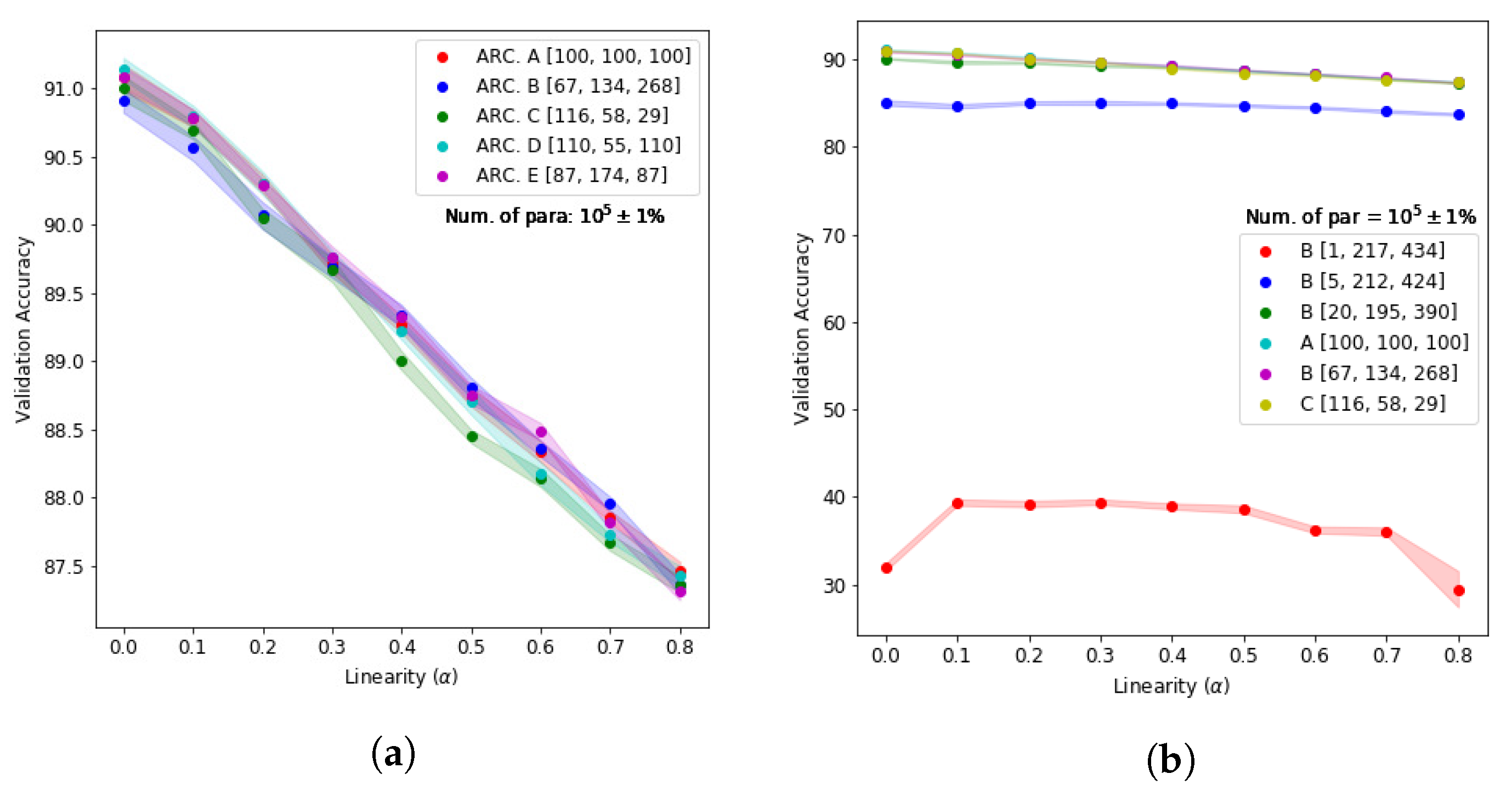
Appendix A.1. Accuracy vs. Linearity Factor for Different Model Architectures with Number of Parameters Fixed

Figure A1. (a) The validation accuracy for different model architectures as a function of linearity factor ( α ) while maintaining the number of parameters fixed ( 10 5 ± 1%). (b) The average validation accuracy as a function of linearity factor ( α ) for the model architectures A, B and C for different number of parameters using 10,000 images from MNIST-digits data set. Shape B was tested for different widths of the first hidden layer while maintaining the number of parameters fixed ( 10 5 ± 1%).
Algorithms 14 00051 g0a1

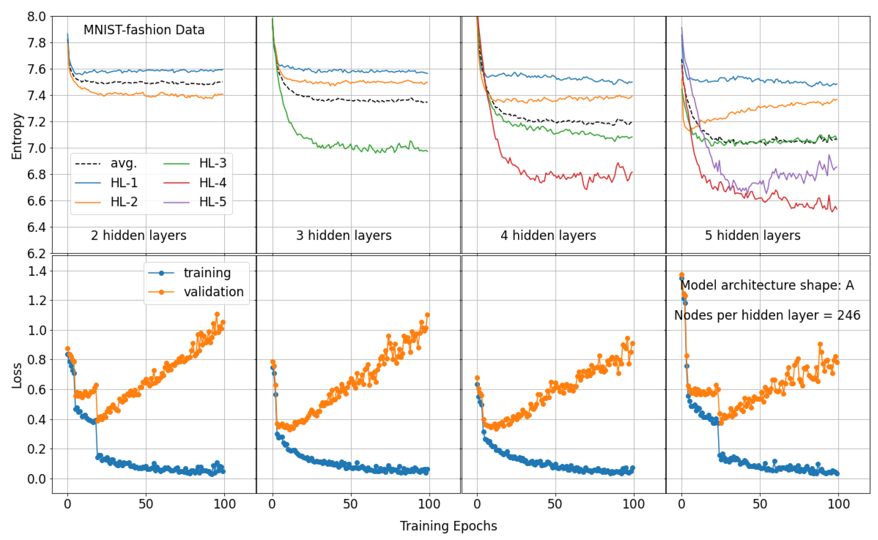
Appendix A.2. Entropy Profile of Model Architecture Shape A Trained Using MNIST-Fashion Data

Figure A2. First row of figures show the entropy profile of four different shallow neural networks. Second row shows the corresponding training and validation losses. These models were trained using 60,000 MNIST-fashion images with 33% validation split. NLLLoss [41] was used as the loss function and the Adam optimizer [42] with learning rate 0.001 was used for the model optimization.
Algorithms 14 00051 g0a2

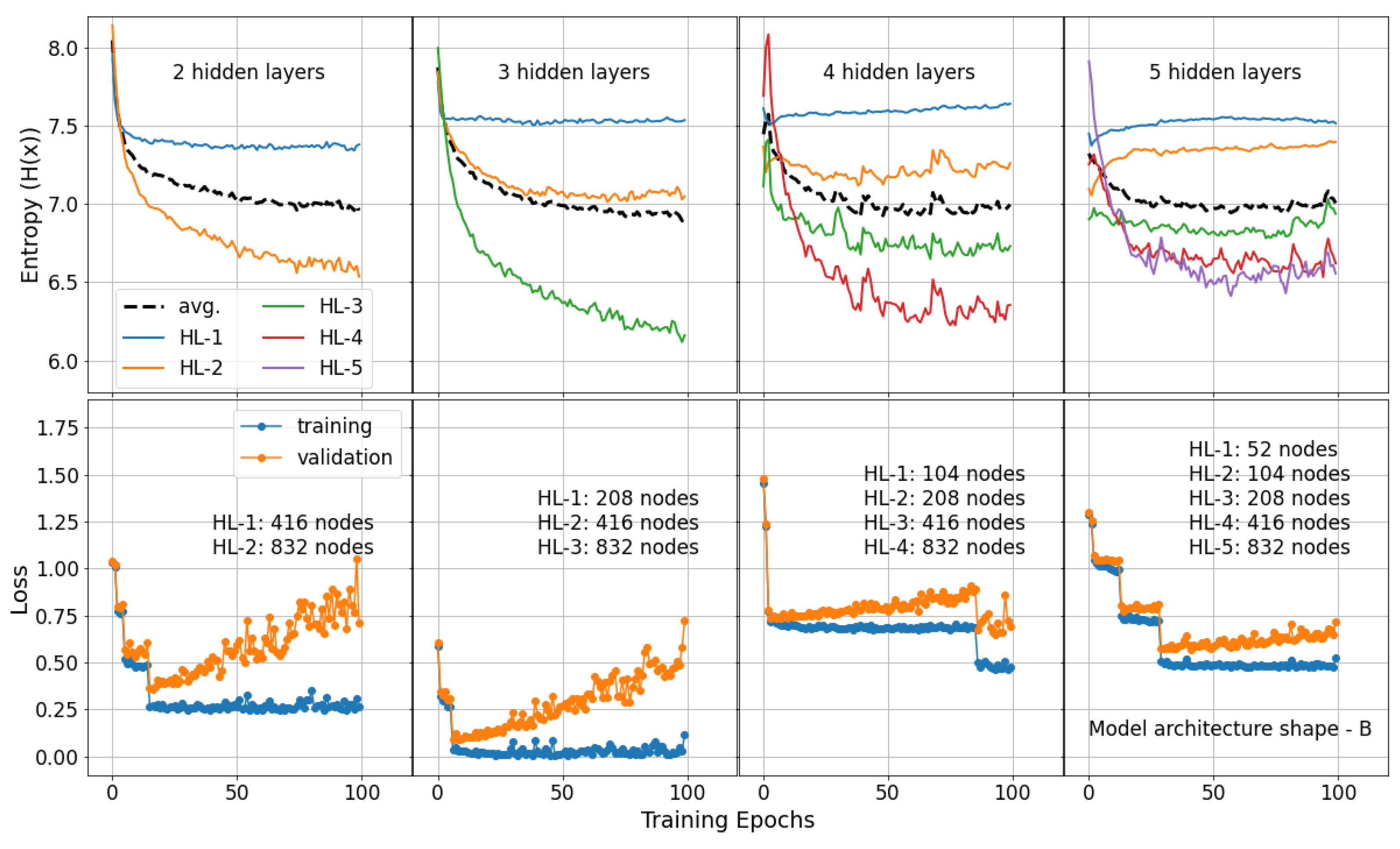
Appendix A.3. Entropy Profile of Model Architecture Shape B Trained Using MNIST-Fashion Data

Figure A3. First row of figures show the entropy profile of four different shallow neural networks. Second row shows the corresponding training and validation losses. These models were trained using 60,000 MNIST-fashion images with 33% validation split. NLLLoss [41] was used as the loss function and the Adam optimizer [42] with learning rate 0.001 was used for the model optimization.
Algorithms 14 00051 g0a3

Appendix A.4. Model Architectures Used for the Study of the Effects of Nonlinearity on the Model Performance in the Presence of Transfer Learning and Different Data Domains

Table A1 shows the model architecture used in the tests performed using transfer learning (results are shown in Figure 4). More details on the pre-trained models used in this analysis (VGG16, VGG19, InceptionV3, Resnet50 and Xception) can be found in: [36,38,39,40]. Note that the input to the classification model shown in Table A1 is the bottleneck features extracted from the pre-trained model followed by GlobalAveragePooling2D operation. The resulting input shape to the classification layer is: 1 × 512 when the VGG16 was used as the pre-trained model. Furthermore, note that for all transfer learning models used in this analysis, (shown in Figure 4), the architecture of the classification layers is the same and equivalent to the architecture shown in Table A1, except that the input dimension for each model was changed according to the shape of the bottleneck layer of the corresponding pre-trained model while output shape was changed according to the number of classes in the data set. The detailed analysis code used in the extraction of bottleneck features and the classification of the bottleneck features can be found in our github repository (GitHub:https://github.com/nalinda05kl/nonlinear_activations, accessed on 20 December 2020). Note that for cifar10 and Dog Breeds data, learning rate was reduced to 0.01 since fast learning rates resulted in under-fitting.
Table A1. Model Architecture for FOOD-11 classification used in the test for the dependence of model performance on data domain for different linearity factors ( α ). Categorical Cross-entropy loss was used for the loss estimation. Stochastic Gradient Descent (SGD) with learning rate = 0.1 was used as the optimizer.
LAYERSHAPE (in, out)NUM. of PAR.
Layer-1(512, 128)65,664
Layer-2(128, 512)66,048
Layer-3(512, 512)262,656
Layer-4(512, 128)65,664
Output(128, 11)1419
Table A2 and Table A3 show the model architecture shapes used in the study performed to understand the effects of linearity in neural networks on their performance in the presence of different data domains (results are shown in Figure 3).
Table A2. Model Architecture for the regression model for continuous data (simulated as in Equation (3)) used in the test for the dependence of model performance on data domain for different linearity factors ( α ) (Figure 3, left panel). Mean Squared Error (MSE) was used for the loss estimation. Stochastic Gradient Descent (SGD) with learning rate = 0.005 was used as the optimizer.
LAYERSHAPE (in, out)NUM. of PAR.
Layer-1(16, 128)2176
Layer-2(128, 512)66,048
Layer-3(512, 512)262,656
Layer-4(512, 128)65,664
Output(128, 1)129
Table A3. Model Architecture for MNIST-digits, MNIST-fashion and EMNIST-letters classifications used in the test for the dependence of model performance on data domain for different linearity factors ( α ) (Figure 3, right panel). Categorical Cross-entropy loss was used for the loss estimation. Stochastic Gradient Descent (SGD) with learning rate = 0.1 was used as the optimizer.
LAYERSHAPE (in, out)NUM. of PAR.
Layer-1(784, 128)100,480
Layer-2(128, 512)66,048
Layer-3(512, 512)262,656
Layer-4(512, 128)65,664
Output(128, 10)1290
In Table A2, the input dimension for the first layer was changed according to the number of features in the continuous data (8, 16 or 24). In Table A3, for EMNIST-letters data, the output layer was changed to 26 nodes (for 26 classes in the data set) while for MNIST-digits and MNIST-fashion data it was 10.

References

  1. Pedamonti, D. Comparison of non-linear activation functions for deep neural networks on MNIST classification task. arXiv 2018, arXiv:1804.02763. [Google Scholar]
  2. Nwankpa, C.; Ijomah, W.; Gachagan, A.; Marshall, S. Activation Functions: Comparison of trends in Practice and Research for Deep Learning. arXiv 2018, arXiv:1811.03378. [Google Scholar]
  3. Xu, B.; Wang, N.; Chen, T.; Li, M. Empirical Evaluation of Rectified Activations in Convolutional Network. arXiv 2015, arXiv:1505.00853. [Google Scholar]
  4. Nair, V.; Hinton, G.E. Rectified Linear Units Improve Restricted Boltzmann Machines. In Proceedings of the 27th International Conference on Machine Learning, ICML’10, Haifa, Israel, 21–24 June 2010; Omnipress: Madison, WI, USA, 2010; pp. 807–814. [Google Scholar]
  5. Arora, R.; Basu, A.; Mianjy, P.; Mukherjee, A. Understanding Deep Neural Networks with Rectified Linear Units. arXiv 2016, arXiv:1611.01491. [Google Scholar]
  6. Javid, A.M.; Das, S.; Skoglund, M.; Chatterjee, S. A ReLU Dense Layer to Improve the Performance of Neural Networks. arXiv 2020, arXiv:2010.13572. [Google Scholar]
  7. Pascanu, R.; Mikolov, T.; Bengio, Y. On the Difficulty of Training Recurrent Neural Networks. In Proceedings of the 30th International Conference on Machine Learning, ICML, Atlanta, GA, USA, 17–19 June 2013. [Google Scholar]
  8. Maas, A.L. Rectifier Nonlinearities Improve Neural Network Acoustic Models. In Proceedings of the 30th International Conference on Machine Learning (ICML), Atlanta, GA, USA, 17–19 June 2013. [Google Scholar]
  9. D’Souza, R.N.; Huang, P.Y.; Yeh, F.C. Structural Analysis and Optimization of Convolutional Neural Networks with a Small Sample Size. Sci. Rep. 2020, 10, 834. [Google Scholar] [CrossRef]
  10. Glorot, X.; Bordes, A.; Bengio, Y. Deep Sparse Rectifier Neural Networks. In Proceedings of the Fourteenth International Conference on Artificial Intelligence and Statistics, Fort Lauderdale, FL, USA, 11–13 April 2011; Volume 15, pp. 315–323. [Google Scholar]
  11. LeCun, Y.; Bengio, Y.; Hinton, G. Deep Learning. Nature 2015, 521, 436–444. [Google Scholar] [CrossRef] [PubMed]
  12. Panigrahi, A.; Shetty, A.; Goyal, N. Effect of Activation Functions on the Training of Overparametrized Neural Nets. arXiv 2020, arXiv:1908.05660. [Google Scholar]
  13. Hahnloser, R.; Sarpeshkar, R.; Mahowald, M.; Douglas, R.; Seung, S. Digital selection and analogue amplification coexist in a cortex-inspired silicon circuit. Nature 2000, 405, 947–951. [Google Scholar] [CrossRef] [PubMed]
  14. Feurer, M.; Klein, A.; Eggensperger, K.; Springenberg, J.; Blum, M.; Hutter, F. Efficient and Robust Automated Machine Learning. In Advances in Neural Information Processing Systems; Cortes, C., Lawrence, N., Lee, D., Sugiyama, M., Garnett, R., Eds.; Curran Associates, Inc.: Red Hook, NY, USA, 2015; Volume 28, pp. 2962–2970. [Google Scholar]
  15. Hutter, F.; Hoos, H.; Leyton-Brown, K. An Efficient Approach for Assessing Hyperparameter Importance. In Proceedings of the 31st International Conference on Machine Learning ICML, Beijing, China, 21–26 June 2014. [Google Scholar]
  16. Probst, P.; Bischl, B.; Boulesteix, A.L. Tunability: Importance of Hyperparameters of Machine Learning Algorithms. arXiv 2018, arXiv:1802.09596. [Google Scholar]
  17. van Rijn, J.N.; Hutter, F. Hyperparameter Importance Across Datasets. In Proceedings of the 24th ACM SIGKDD International Conference on Knowledge Discovery & Data Mining, London, UK, 19–23 August 2018. [Google Scholar] [CrossRef] [Green Version]
  18. Chen, B.; Zhang, K.; Ou, L.; Ba, C.; Wang, H.; Wang, C. Automatic Hyper-Parameter Optimization Based on Mapping Discovery from Data to Hyper-Parameters. arXiv 2020, arXiv:2003.01751. [Google Scholar]
  19. Lee, A.; Xin, D.; Lee, D.; Parameswaran, A. Demystifying a Dark Art: Understanding Real-World Machine Learning Model Development. arXiv 2020, arXiv:2005.01520. [Google Scholar]
  20. Khan, A.; Sohail, A.; Zahoora, U.; Qureshi, A.S. A survey of the recent architectures of deep convolutional neural networks. Artif. Intell. Rev. 2020, 53, 5455–5516. [Google Scholar] [CrossRef] [Green Version]
  21. Lu, L.; Shin, Y.; Su, Y.; Karniadakis, G.E. Dying ReLU and Initialization: Theory and Numerical Examples. arXiv 2019, arXiv:1903.06733. [Google Scholar] [CrossRef]
  22. Sperl, P.; Böttinger, K. Optimizing Information Loss Towards Robust Neural Networks. arXiv 2020, arXiv:2008.03072. [Google Scholar]
  23. Foggo, B.; Yu, N.; Shi, J.; Gao, Y. Information Losses in Neural Classifiers From Sampling. IEEE Trans. Neural Networks Learn. Syst. 2020, 31, 4073–4083. [Google Scholar] [CrossRef]
  24. LeCun, Y.; Cortes, C. MNIST Handwritten Digit Database. 2010. Available online: http://yann.lecun.com/exdb/mnist/ (accessed on 10 October 2020).
  25. Xiao, H.; Rasul, K.; Vollgraf, R. Fashion-MNIST: A Novel Image Dataset for Benchmarking Machine Learning Algorithms. arXiv 2017, arXiv:1708.07747. [Google Scholar]
  26. Cohen, G.; Afshar, S.; Tapson, J.; Schaik, A.V. EMNIST: Extending MNIST to handwritten letters. In Proceedings of the 2017 International Joint Conference on Neural Networks (IJCNN), Anchorage, AK, USA, 14–19 May 2017. [Google Scholar] [CrossRef]
  27. Pedregosa, F.; Varoquaux, G.; Gramfort, A.; Michel, V.; Thirion, B.; Grisel, O.; Blondel, M.; Prettenhofer, P.; Weiss, R.; Dubourg, V.; et al. Scikit-learn: Machine learning in Python. J. Mach. Learn. Res. 2011, 12, 2825–2830. [Google Scholar]
  28. Chollet, F. Keras: The Python Deep Learning API. 2015. Available online: https://github.com/fchollet/keras (accessed on 10 January 2021).
  29. Paszke, A.; Gross, S.; Massa, F.; Lerer, A.; Bradbury, J.; Chanan, G.; Killeen, T.; Lin, Z.; Gimelshein, N.; Antiga, L.; et al. PyTorch: An Imperative Style, High-Performance Deep Learning Library. In Advances in Neural Information Processing Systems 32; Curran Associates, Inc.: Red Hook, NY, USA, 2019; pp. 8024–8035. [Google Scholar]
  30. Nystrom, N.A.; Levine, M.J.; Roskies, R.Z.; Scott, J.R. Bridges: A Uniquely Flexible HPC Resource for New Communities and Data Analytics. In Proceedings of the 2015 XSEDE Conference: Scientific Advancements Enabled by Enhanced Cyberinfrastructure, XSEDE ’15, St. Louis, MO, USA, 26–30 July 2015; ACM: New York, NY, USA, 2015; pp. 30:1–30:8. [Google Scholar] [CrossRef]
  31. Ruder, S. An overview of gradient descent optimization algorithms. arXiv 2016, arXiv:1609.04747. [Google Scholar]
  32. Mannor, S.; Peleg, D.; Rubinstein, R. The cross entropy method for classification. In Proceedings of the 22nd International Conference on Machine Learning, Bonn, Germany, 7–11 August 2005; pp. 561–568. [Google Scholar] [CrossRef] [Green Version]
  33. Singla, A.; Yuan, L.; Ebrahimi, T. Food/Non-food Image Classification and Food Categorization using Pre-Trained GoogLeNet Model. In Proceedings of the 2nd International Workshop on MADiMa, Amsterdam, The Netherlands, 16 October 2016; pp. 3–11. [Google Scholar] [CrossRef] [Green Version]
  34. Krizhevsky, A. Learning Multiple Layers of Features from Tiny Images. 2009. Available online: https://www.cs.toronto.edu/~kriz/cifar.html (accessed on 15 January 2021).
  35. Liu, J.; Kanazawa, A.; Jacobs, D.; Belhumeur, P. Dog Breed Classification Using Part Localization. In Computer Vision—ECCV; Springer: Berlin/Heidelberg, Germany, 2012; pp. 172–185. [Google Scholar]
  36. Simonyan, K.; Zisserman, A. Very Deep Convolutional Networks for Large-Scale Image Recognition. arXiv 2015, arXiv:1409.1556. [Google Scholar]
  37. Russakovsky, O.; Deng, J.; Su, H.; Krause, J.; Satheesh, S.; Ma, S.; Huang, Z.; Karpathy, A.; Khosla, A.; Bernstein, M.; et al. ImageNet Large Scale Visual Recognition Challenge. Int. J. Comput. Vis. IJCV 2015, 115, 211–252. [Google Scholar] [CrossRef] [Green Version]
  38. Szegedy, C.; Vanhoucke, V.; Ioffe, S.; Shlens, J.; Wojna, Z. Rethinking the Inception Architecture for Computer Vision. arXiv 2015, arXiv:1512.00567. [Google Scholar]
  39. He, K.; Zhang, X.; Ren, S.; Sun, J. Deep Residual Learning for Image Recognition. arXiv 2015, arXiv:1512.03385. [Google Scholar]
  40. Chollet, F. Xception: Deep Learning with Depthwise Separable Convolutions. arXiv 2017, arXiv:1610.02357. [Google Scholar]
  41. The Negative Log Likelihood Loss. Available online: https://pytorch.org/docs/stable/generated/torch.nn.NLLLoss.html (accessed on 10 December 2020).
  42. Kingma, D.P.; Ba, J.L. Adam: A Method for Stochastic Optimization. arXiv 2017, arXiv:1412.6980. [Google Scholar]
  43. Kullback, S.; Leibler, R.A. On Information and Sufficiency. Ann. Math. Statist. 1951, 22, 79–86. [Google Scholar] [CrossRef]
  44. Joyce, J.M. Kullback-Leibler Divergence. In International Encyclopedia of Statistical Science; Lovric, M., Ed.; Springer: Berlin/Heidelberg, Germany, 2011; pp. 720–722. [Google Scholar] [CrossRef]
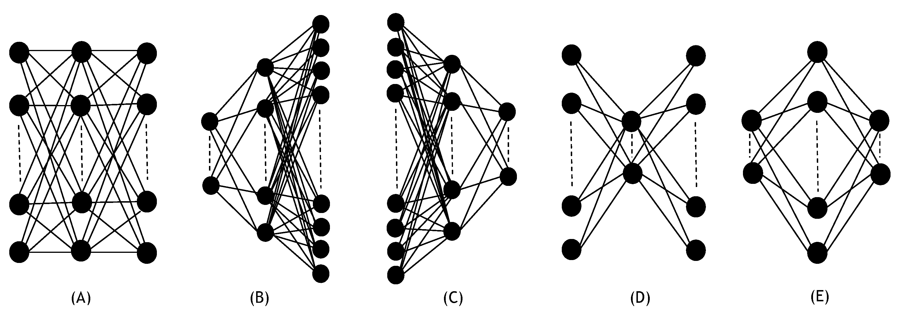
Figure 1. Illustrations in (AE) are the five model architecture shapes used in the analysis. For each architecture shape, number of nodes per hidden layer was varied according to Table 1, in order to change the model complexity.
Algorithms 14 00051 g001
Figure 2. The maximum validation accuracy as a function of the linearity factor ( α ) for models with five network architecture shapes (Arch. shapes A–E) and three network widths (see Table 1). Models were trained on 20,000 MNIST-digits images (upper panel) and 20,000 MNIST-fashion images (lower panel). For all the models used in this test, the number of nodes used in each hidden layer is shown within the square brackets in each sub-figure in the order of number of nodes used in first, second and third hidden layers, respectively.
Algorithms 14 00051 g002
Figure 3. (left panel) Validation loss as a function of linearity factor ( α ) for continuous data with different dimensions: 8, 16 and 24 features (ft.). (right panel) Training and validation loss as a function of linearity factor ( α ) for categorical data (MNIST-digits, MNIST-fashion and EMNIST-letters data sets). Note that, to test the effects of data domains, a neural network with a fixed architecture shape was used in the modeling of all data sets shown in this figure. (see Appendix A.4, Table A2 and Table A3) for model details.
Algorithms 14 00051 g003
Figure 4. (a) Validation loss with respect to the validation loss at α = 0 as a function of linearity factor ( α ) for Dog Breeds, FOOD-11 and cifar10 data sets modeled using VGG16 pre-trained model, (b) validation loss with respect to the validation loss at α = 0 as a function of linearity factor ( α ) for Dog Breeds data using VGG16, VGG19, InceptionV3, ResNet50 and Xception pre-trained models. For each curve, width of the band shows the uncertainty due to different weight initialization in classification layers.
Algorithms 14 00051 g004
Figure 5. Entropy profile for the 5-layer neural network during the training process. Linearity factor ( α ) in L-ReLU was changed from α = 0.0 to α = 0.4 . Hidden layers 1–5 of the neural network consist of nodes combinations: 256, 128, 128, 128 and 32, respectively. This test was done using two different data sets, 60,000 MNIST-digits images (upper panel) and MNIST-fashion images (lower panel) with 33% validation split. Black curves show the average (avg.) entropy in the network.
Algorithms 14 00051 g005
Figure 6. First row of figures show the entropy profile of four different shallow neural networks. Second row shows the corresponding training and validation losses. Number of hidden layes were changed from two to five and each hidden layer (HL) consist of 246 nodes. Note that the black curves in the first row of figures show the average (avg.) entropy of each model. These models were trained using 60,000 MNIST-digits images with 33% validation split. NLLLoss [41] was used as the loss function and the Adam optimizer [42] with learning rate 0.001 was used for the model optimization.
Algorithms 14 00051 g006
Figure 7. First row of figures show the entropy profile of four different shallow neural networks. Second row shows the corresponding training and validation losses. Number of hidden layers were changed from two to five. The number of nodes in each hidden layer (HL) of these models are printed in each sub-figure of second raw. Note that the black curves in the first row of figures show the average (avg.) entropy of each model. These models were trained using 60,000 MNIST-digits images with 33% validation split. NLLLoss [41] was used as the loss function and the Adam optimizer [42] with learning rate 0.001 was used for the model optimization.
Algorithms 14 00051 g007
Table 1. Different combinations of number of nodes used in three hidden layers of the five network Architecture shapes A–E (Arch. A–E) presented in in Figure 1. Width of each model architecture shape was varied by changing the number of nodes per layer. For each model architecture, the number of nodes used is shown as, ( n 1 , n 2 , n 3 ) and they represent the number of nodes in first, second and third hidden layers, respectively.
WidthArch. AArch. BArch. CArch. DArch. E
width-1(8, 8, 8)(8, 16, 32)(16, 8, 4)(16, 8, 16)(8, 16, 8)
width-2(32, 32, 32)(32, 64, 128)(64, 32, 16)(64, 32, 64)(32, 64, 32)
width-3(256, 256, 256)(128, 256, 512)(512, 256, 128)(512, 256, 512)(256, 512, 256)
Table 2. Optimal value of the linearity factor ( α ) at which the maximum validation accuracy was achieved for neural network models tested using MNIST-digits and MNIST-fashion images. Width of each model architecture shape was varied by changing the number of nodes per layer. See Table 1 for the number of nodes per layer corresponding to the network widths used in each model.
TrainingWidthOptimal Valve of the Linearity ( α ) in the Network
Data Setper LayerArch. AArch. BArch. CArch. DArch. E
MNIST-width-10.30.30.20.10.5
digitswidth-20.00.10.00.00.0
width-30.00.00.00.00.0
MNIST-width-10.40.30.10.10.5
fashionwidth-20.10.10.10.00.1
width-30.10.00.10.00.0
Publisher’s Note: MDPI stays neutral with regard to jurisdictional claims in published maps and institutional affiliations.

