
Adaptive Quick Reduct for Feature Drift Detection


Department of Science and Technologies, University of Naples “Parthenope”, Centro Direzionale Napoli, Isola C4, I-80143 Napoli, Italy
*
Author to whom correspondence should be addressed.
Algorithms 2021, 14(2), 58; https://0-doi-org.brum.beds.ac.uk/10.3390/a14020058
Submission received: 6 January 2021
/
Revised: 2 February 2021
/
Accepted: 8 February 2021
/
Published: 11 February 2021
(This article belongs to the Special Issue Granular Computing: From Foundations to Applications)
Abstract
:Data streams are ubiquitous and related to the proliferation of low-cost mobile devices, sensors, wireless networks and the Internet of Things. While it is well known that complex phenomena are not stationary and exhibit a concept drift when observed for a sufficiently long time, relatively few studies have addressed the related problem of feature drift. In this paper, a variation of the QuickReduct algorithm suitable to process data streams is proposed and tested: it builds an evolving reduct that dynamically selects the relevant features in the stream, removing the redundant ones and adding the newly relevant ones as soon as they become such. Tests on five publicly available datasets with an artificially injected drift have confirmed the effectiveness of the proposed method.
1. Introduction
The analysis of data streams is challenging in many ways: being the data a continuous flux of information, only a small fraction of it can be processed; older data lose significance and newer data can change their behavior suddenly; answers are required almost in real time and computational resources are an issue, even when the data are buffered (please see [1] for a general review and [2] for a more specific focus on Machine Learning). Both clustering and classification require efficient evolving strategies in order to cope with these issues, and Feature Selection (FS from now on) is a key component in order to reduce the dimensionality, to lower the computational burden and hence to increase the effectiveness of the chosen classification or clustering algorithms.
The data stream typically comes from multiple sensors that produce numerical data. The incoming sources can be seen as the realization of a multivariate random variable dependent on time or a collection of univariate random variables with different distributions, each of which can be called dimension or feature. Without loss of generality, for a fixed number of sources, the stream can be seen as a non-finite sequence of vectors of size r, where r is the number of sources (or variables or dimensions or features):
1.1. Windowing
As streaming data are discrete but by definition infinite, it is common to use a window model to analyze them, as a compromise between real-time and full batch processing. Memory and time constraints obviously limit the width of the window, for which four common models exist: sliding, damped, landmark and tilted (please see [1] for a review).
- Sliding windows are the classic model where the most recent d observations are considered, with a fixed overlap of o observations between a window and the next;
- Damped windows are a model where data receive a decreasing weight through a decay function (usually exponential) as they age, reducing progressively their relevance;
- Landmark windows are consecutive windows separated by special observation called landmarks, with no overlap between a window and the next;
- Tilted windows are windows whose width increases with the age of the observations, following the principle that newer observations require a finer level of detail.
1.2. Concept Drift
The concept drift happens when the distribution underlying the data stream is non-stationary. It is a broad term that may refer to four different situations according to the related Literature (please see [3] for a comprehensive review):
- Sudden drift (also called concept shift), it is the case when in a very short period of time a new concept replaces the previous one, that is the probability distribution changes abruptly;
- Gradual drift, that happens when in a moderately long period of time the occurrences of the new concept contaminate gradually the old one, until they replace the old concept completely and the new probability distribution prevails;
- Incremental drift (or morphing), that happens when there is a smooth, gradual transition from the old concept to the new one, that is the instances gradually and continuously move from the old concept to the new one;
- Reoccurring drift, that happens when an old concept reappears after a shift, with unknown periodicity. It may become a reoccurring shift if the transition is abrupt.
1.3. Feature Drift
Analogously, and relatedly, feature drift is defined as the change of relevance of a feature over time. It comes into play when a feature selection algorithm is used on a data stream, where the non-stationarity of the phenomenon produces a variable subset of best features for classification as times passes. Compared to concept drift, feature drift has emerged only recently and few techniques have been developed so far (please see [4] for a review). It must be stressed that feature drift can be captured with dynamic feature selection methods, as proposed in this paper, but that it is different from Online Feature Selection or Streaming Feature Selection methods: the latter involve learning on a stream of features, not instances (please see [5,6] for further details and an example of techniques based on Rough Sets).
The relevance of a feature f in a Feature Selection problem can be expressed by a function, that in the simplest cases has a binary codomain:
the relevance function, can also have a continuous codomain in more sophisticated cases:
where ultimately a threshold function T is often used to establish which feature should be finally included in the reduced set.
So without loss of generality can be used for both cases. The relevance of a feature is related to its prediction power with respect to the target classes.
The redundancy of a feature f in a Feature Selection problem can be expressed by a function, that in the simplest cases may be a simple linear correlation coefficient with other features. A feature is considered redundant if its prediction power is absorbed by the feature already in the best set, in other terms if the prediction power of the best set of feature does not change removing this feature from it.
Again, four types of drift can be observed, but using windows instead of single instances as references for time and in the context of a classification problem:
- Sudden drift (also called feature shift), it is the case when in in two consecutive time windows a feature becomes irrelevant or redundant (and should be excluded from the best set of features) or relevant (and should be added to the best set of features) for classification, remaining in that state for a certain number of consecutive windows;
- Gradual drift, that happens when considering a number of consecutive time windows the frequency of a feature resulting relevant (irrelevant) increases (decreases) over time: it is a situation when a feature at first appears and disappears intermittently from the set of relevant features—it is on the edge of relevance—and then stabilizes itself;
- Incremental drift (or morphing), that happens when the relevance of a feature between a number of consecutive time windows is expressed by a continuous number in that increases (or decreases) monotonically;
- Reoccurring drift, that happens when a feature that has become irrelevant turns back to be relevant and vice versa, with unknown periodicity. It may become a reoccurring shift if the transition is abrupt.
Furthermore, for feature drift, as for concept drift, it holds the stability-plasticity dilemma: the shorter the time windows are, the more flexible the model is, the most sensitive to noise and the fastest adaptation to drift—eventually spurious—it shows; the longer the time windows are, the more stable the model is, the less sensitive to noise and the slowest adaptation to the—eventually actual—drift it shows. Reoccuring drift/shift can be included in the other three cases given enough plasticity of the model, while gradual and incremental drift may easily coexist in longer time windows.
An adaptation of QuickReduct to streaming data, able to recognize feature shift and to remove redundant features at the same time is proposed in the following.
2. Materials and Methods
The required background notions on Rough Sets, Feature Selection and QuickReduct are outlined hereafter, followed by the detailed description of the proposed AdaptiveQuickReduct algorithm and its limitations.
2.1. QuickReduct for Feature Selection
Let U be the universe of discourse and A be a finite set of attributes; let be an information system: an equivalence relation in I is the set of objects belonging to U that are not discernible by attributes in P, defined as follows:
It can represent any , where each attribute A has values in , such that , .
Every equivalence relation defines a partition set of U, called , that splits U in equivalence classes called [7]. According to [8], equivalence classes correspond to information granules and can be used to approximate any subset through a pair: its lower approximation (Equation (7)) and its upper approximation (Equation (8)).
The positive region—given two equivalence relations called C and D over U—is defined as:
and represents the union of the lower approximations of all the equivalence classes defined by . From the definition of the positive region it is possible to derive the degree of dependency of a set of attributes D on a set of attributes C, called :
A reduct is the subset of minimal cardinality of the set of conditional attribute C such that its degree of dependency remains unchanged:
where is the set of decision features and is the set of conditional attributes.
A reduct is minimal, meaning that no attribute can be removed from the reduct itself without lowering its dependency degree with the full set of conditional attributes. Most of the feature selection algorithms used in Rough Set theory are based on the definition of reduct and on the efficient construction of the optimal reduct [9,10,11,12].
The QuickReduct [13] (please see Algorithm 1, called QR from now on) builds the reduct concatenating the attributes with the greatest increase in the dependency degree, up to its maximum in the considered dataset. Being the exploration of all possible feature combinations computationally unfeasible, QR uses a greedy choice: it adds one at a time to the empty set the attributes resulting in the greatest increase in the Rough Set dependency degree until no other attribute can be added. In this way, it is not guaranteed to find the optimal minimum number of features, however it derives a subset sufficiently close to optimal in a reasonable time, resulting in general a good compromise between time and performance to reduce the dataset dimensionality in many real world scenarios [14].
| Algorithm 1 QuickReduct |
|
2.2. Adaptive QuickReduct
In order to exploit the idea underlying QuickReduct in an evolving scenario, it is necessary both to detect feature drifts and to change the selected features accordingly. The ideal algorithm should not only add new features that increase the dependency degree of the selected reduct as new data are processed, but also remove the previously selected features whose contribution is no longer relevant.
A typical approach to analyze data streams consists in choosing a windowing model and processing data in each windows, with a moderate overlap between consecutive windows.
Assuming that a reduct is available at time in the window , the goal is to evaluate whether the features remain those with the highest dependency degree with respect to at time and in the window , i.e., if ) or if there is a new better subset .
Two steps are needed: first the removal of the redundant features in and then the addition of new features that increase the dependency degree for . The proposed algorithm, called AdaptiveQuickReduct (AQR from now on) implements exactly this strategy: given a reduct calculated in the time window , the first step iteratively removes all the features such that . The output of this step is a new reduct to be eventually expanded with new features. In particular, let be the set of features removed from , the second step consists in trying to add new features to following the QuickReduct schema. Pseudocode for AQR is reported in Algorithm 2, while Algorithm 3 reports a driver program that acts as a detector and shows how AQR can be called with a sliding window, in which parameter W represents the window size (batch) that moves forward by O instances at each iteration.
| Algorithm 2 AdaptiveQuickReduct |
|
| Algorithm 3 FeatureDriftDetection |
|
Although it is possible to detect gradual or incremental drift considering a thresholding function T, the definition of a continuous relevance score would be required, which is not explicitly available in QR as it does not give a weight to the features to be selected. On the contrary, the sudden change that occurs at a precise moment—feature shift—is easily detectable through a qualitative analysis of the output.
As stated in Section 2.1, a minimal reduct is a subset of the dataset conditional features that has equal rough dependency degree as the full set of features and such that no strict subset of this reduct exists that has a greater dependency degree. It must be stressed that the variation in dependency degree given by the addition or deletion of a single feature, even though effective, does not guarantee to predict the optimal reduct, but in general a super-reduct (a subsets that has maximal dependency but not the smallest cardinality). This limitation is in common with QR and it is due to their greedy nature, consequence of the unfeasibility of exhaustive search for the optimal reduct [15]. Nonetheless, as proven by the successful application of QR in countless domains, even the sub–optimal reduct is a sufficiently good approximation in most real world application (see for example [16]).
Other approaches to Feature Drift detection are Dynamic Feature Weighting (DRW, see [17]), where the weight of each feature is increased or diminished according to its relevance obtained through entropy or symmetrical uncertainty on sliding windows; or methods based on Hoeffding Trees (see [18]), that is Decision Trees that use the Hoeffding bound to compute an arbitrarily close to optimal Decision Trees on the base of a limited amount of streaming data (see [19,20,21]). Even ensembles have been proposed to extend methods based on Hoeffding Trees, at the cost of an higher computational burden [22]. To the best of our knowledge, none of these exploits fuzziness or roughness in detecting drifts.
3. Results
The experimental framework and the performances obtained by the proposed algorithm in detecting feature shift are reported hereafter. Publicly available datasets have been chosen and modified artificially inserting shifts in predefined positions for testing purposes. For each test plots of the selected features at each iteration are shown at the end of the section.
3.1. Data
The datasets used in the experiments are all publicly available from the UCI Machine Learning repository [23]. Their names and main characteristics are summarized in Table 1. To emulate a stream, data are processed in a First-In First-Out (FIFO) order considering their record number as the key of a sorted file.
3.2. Drift Injection
Each reduct represents the set of selected features in its time window. To benchmark the ability of AQR to detect the feature shift and redefine the reduct accordingly, the exact moment in which the shift occurs in each dataset shall be known in advance.
To this end, the distributions of some features in a predefined position of the dataset have been modified swapping their values. The feature to be swapped are chosen so that one is among the most relevant and the other is among the least relevant according to QR executed in full batch mode. Table 2 reports the drift insert points on the selected datasets.
3.3. Tests
Four different tests have been performed to evaluate the effectiveness of AQR in different conditions of shift and feature dependence and a fifth test has been performed to evaluate its effectiveness in improving classification.
3.3.1. Test 1. Simple Shift
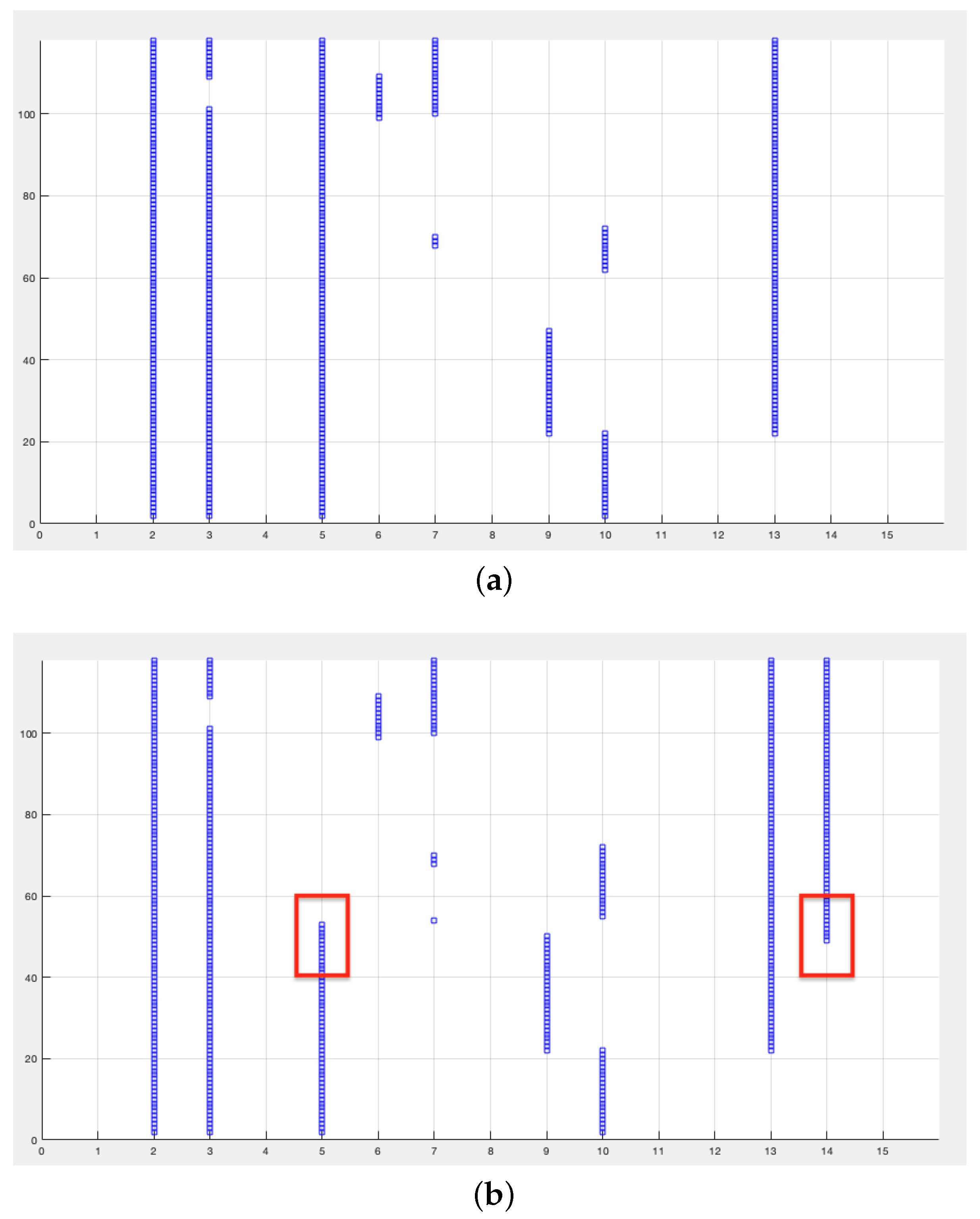
The first test aims to evaluate the ability of AQR to actually recognize a feature shift: features 5 and 14 are swapped starting from observation 300 to the end of the file. The window is fixed at 100 observations and the overlap between a window and the next is 95 observations. With these parameters the drift occurs at the 40th iteration. Figure 1 shows the graphs of the selected features at each iteration without drift (a) and with drift highlighted in red (b).
Regarding feature five, the detection occurs at iteration 53 with a delay of 13 iterations (65 observations) while the drift detection on feature 14 occurs at iteration 49 with a delay of only 9 iterations (45 observations). From the comparison with the selected features without drift, it is possible to appreciate the stability of the proposed algorithm.
3.3.2. Test 2. Reoccurring Shift
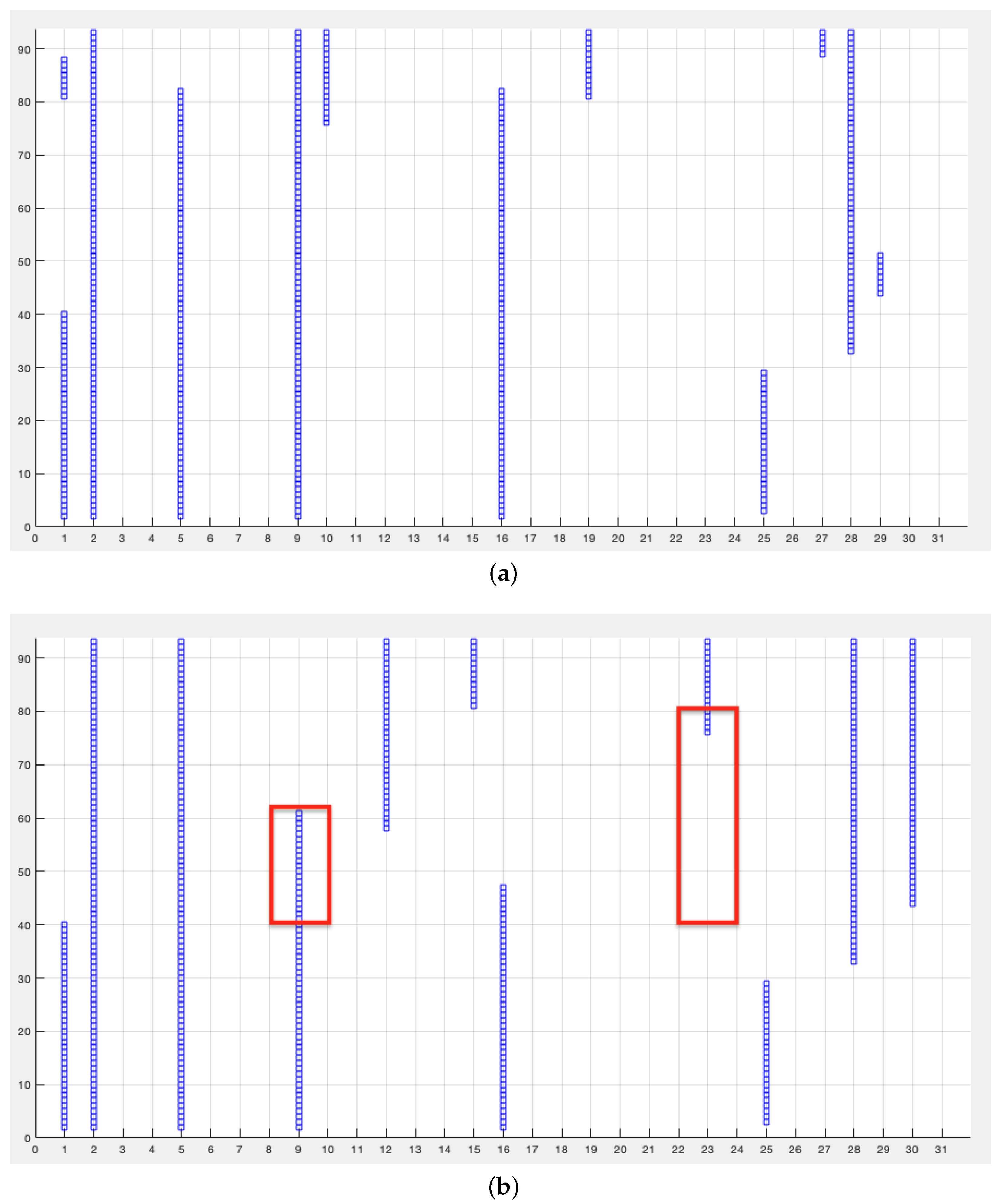
The the second test aims to evaluate the ability of AQR to recognize reoccurring shift. To this purpose, features 5 and 14 have been swapped only from observation 300 to 400. The window is fixed at 100 observations and the overlap is 95 observations. With these parameters the drift occurs from the 40th to the 60th iteration. Figure 2 shows the plots of the selected features at each iteration without drift (a) and with drift highlighted in red (b).
As for feature 5, the initial detection occurs at iteration 53 with a delay of 13 iterations (65 observations) while the final detection occurs at iteration 72 with a delay of 12 iterations (60 observations), therefore the algorithm shows a response-time equal to circa half of the window to detect the drift (temporarily removing feature 5). As for feature 14, the initial detection occurs at iteration 49 with a delay of only nine iterations (45 observations) while the final detection occurs at iteration 85 with a delay of 25 iterations (125 observations).
3.3.3. Test 3. Shift with Partially Dependent Features
The dataset used in the third test has a larger number of features. The specificity of this dataset with respect to QR is that the degree of dependence of the complete set of features never reaches unity and in many cases is less than 0.8 (Figure 3).
Furthermore, the low fraction of selected features indicates that many of them are redundant, non-discriminative and actually worsen performances. In this test, features 9 and 13 were swapped from observation 300 to the end of the dataset. The window is fixed to 100 observations and the overlap is of 95 observations, so the drift occurs at the 40th iteration. Figure 4 shows the plots of the selected features at each iteration without drift (a) and with drift highlighted in red (b).
As for feature 9, the detection occurs at iteration 60 with a delay of 20 iterations (100 observations) while the drift detection on feature 23 occurs at iteration 76 with a delay of 36 iterations (180 observations). From this test it is evident that the detection accuracy is strongly related to the discriminating power of the features.
3.3.4. Test 4. Shift with Highly Dependent Features
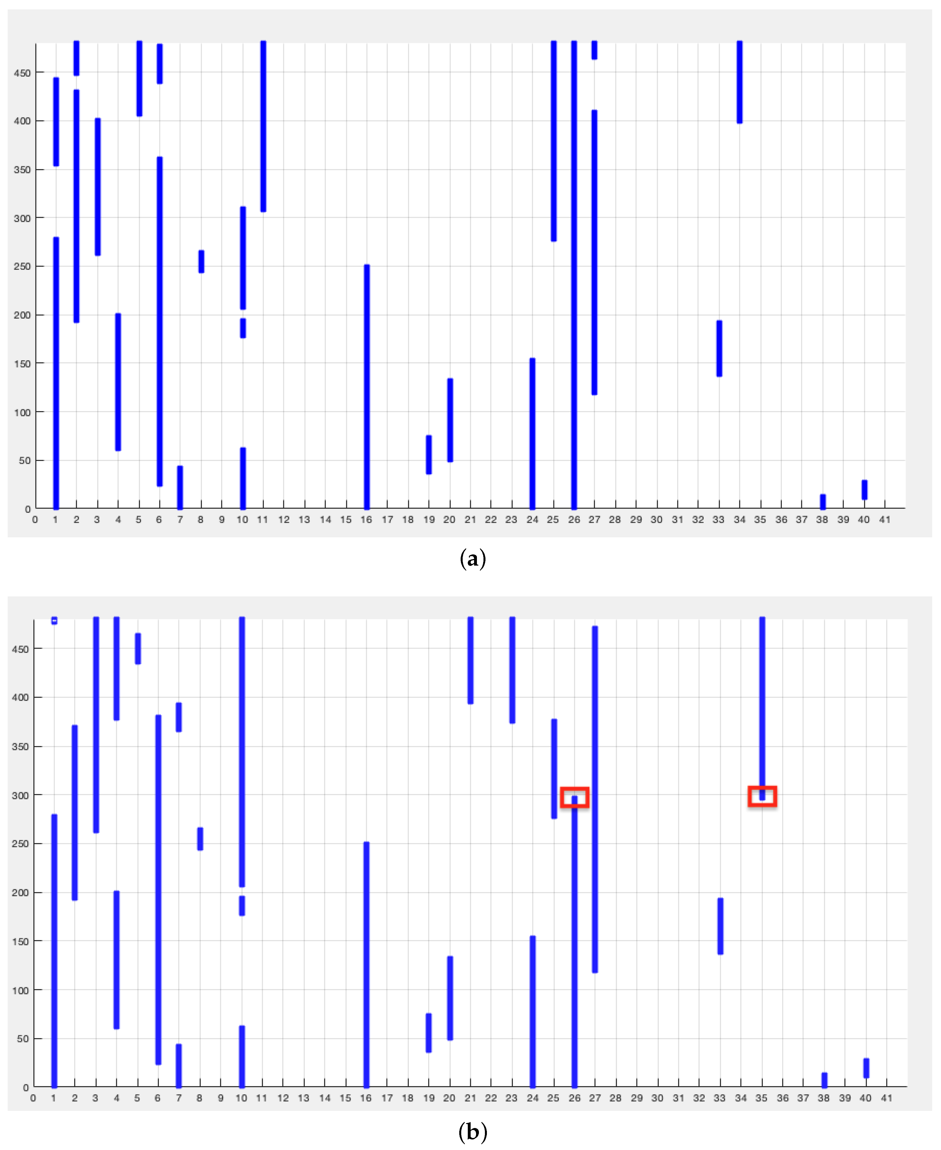
To further investigate this aspect, the fourth test was conducted on a dataset with a larger number of features and observations, where the degree of feature dependency is very high. Features 26 and 35 were swapped from observation 3000 to the end of the dataset. The window is fixed at 200 observations and the overlap is 190 observations, so the drift occurs at the 280th iteration. Figure 5 shows the plots of the selected features at each iteration without drift (a) and with drift highlighted in red (b).
As for feature 26, the detection occurs at iteration 296 with a delay of 16 iterations (80 observations) while the drift detection on feature 35 occurs at iteration 297 with a delay of 17 iterations (85 observations). In this case the algorithm was able to adapt to the drift in less than half of the window.
3.4. Test 5. Classification
In order to further asses the potentialities of AQR, the protocol proposed in [17] and based on prediction accuracy has been adopted. Because AQR is not a classifier but a feature selector, it was paired with k-Nearest Neighbor (kNN) to classify the instances in the current window, obtaining the kNN-AQR combo (very similar results however have been obtained in combination with the Naive Bayes classifier). The accuracy is computed accordingly to the Prequential or interleaved-test-then-train scheme [24], where each instance is first used to test and then to train the model.
The chosen datasets are Electricity [25] and Kaggle’s Give Me Some Credit (GMSC) [26], whose characteristics are summarized in Table 3.
The proposed algorithm is compared with the following competitors: kNN, Naive Bayes, kNN with feature weighting (kNN-FW) [17], Naive Bayes with feature weighing (NB-FW) [17], Very Fast Decision Tree (VFDT) [20] and a Hoeffding Adaptive Tree (HAT) [21].
In Table 4, comparative performances are reported. On the Electricity dataset, the best performing algorithm is kNN-FW that however has the drawback of an higher memory footprint if compared to kNN-AQR (the latter only needs to keep in memory the last computed reduct). Still, kNN-AQR yields a prequential accuracy slightly inferior to HAT, that is one of the best performing algorithms for stream classification with feature drifts. On the other side, on the GMSC dataset, kNN-AQR resulted the best performing algorithm, proving its stability on the long run.
4. Conclusions
Feature drift in data stream is a recent research area that is attracting great interest. In this paper, an effective feature shift detection algorithm based on QuickReduct has been proposed, together with an easily reproducible method to inject drift into a dataset for testing purposes.
The Adaptive QuickReduct has proven to effectively capture the shift artificially injected in three real world datasets under different dependency conditions and to work well in the classification of real world data streams, with a very low memory footprint. While not showing always the best absolute performance in classification and not guaranteeing always the optimal reduct in feature selection, the low memory requirements and the fast response to the eventual shift make it ideal in those application fields where such shift are common and the data volume is high: IoT environments, sensor networks and social media analysis, just to name a few.
Future work will follow two directions: the first is extending the proposed algorithm to deal with gradual and incremental drifts; the second is to hybridize it with leading feature drift frameworks, like VFDT and HAT, in order to further improve their classification performances. Work on a publicly available tool to inject feature drift into a dataset for testing purposes is ongoing.
Author Contributions
Authors contributed equally to the paper. Both authors have read and agreed to the published version of the manuscript.
Funding
This research received no external funding.
Institutional Review Board Statement
Not applicable.
Informed Consent Statement
Not applicable.
Data Availability Statement
Publicly available datasets were analyzed in this study. This data can be found here: http://archive.ics.uci.edu/ml and https://www.kaggle.com/datasets (accessed on 27 December 2020).
Conflicts of Interest
The authors declare no conflict of interest.
References
- Nguyen, H.-L.; Woon, Y.-K.; Ng, W.K. A Survey on Data Stream Clustering and Classification. Knowl. Inf. Syst. 2015, 45, 535–569. [Google Scholar] [CrossRef]
- Gomes, H.M.; Read, J.; Bifet, A.; Barddal, J.P.; Gama, J. Machine learning for streaming data: State of the art, challenges, and opportunities. SIGKDD Explor. Newsl. 2019, 21, 6–22. [Google Scholar] [CrossRef]
- Lu, J.; Liu, A.; Dong, F.; Gu, F.; Gama, J.; Zhang, G. Learning under Concept Drift: A Review. IEEE Trans. Knowl. Data Eng. 2019, 31, 2346–2363. [Google Scholar] [CrossRef] [Green Version]
- Barddal, J.P.; Gomes, H.M.; Enembreck, F.; Pfahringer, B. A survey on feature drift adaptation: Definition, benchmark, challenges and future directions. J. Syst. Softw. 2017, 127, 278–294. [Google Scholar] [CrossRef] [Green Version]
- Sadegh, E.; Javidi, M.M. Online streaming feature selection using rough sets. Int. J. Approx. Reason. 2015, 69, 35–57. [Google Scholar]
- Zhou, P.; Hu, X.; Li, P.; Wu, X. Online streaming feature selection using adapted Neighborhood Rough Set. Inf. Sci. 2019, 481, 258–279. [Google Scholar] [CrossRef]
- Pawlak, Z. Granularity of knowledge, indiscernibility and rough sets. In Proceedings of the IEEE International Conference on Fuzzy Systems, Anchorage, AK, USA, 4–9 May 1998; pp. 106–110. [Google Scholar]
- Pawlak, Z. Rough sets. Int. J. Comput. Inf. Sci. 1982, 11, 341–356. [Google Scholar] [CrossRef]
- Ferone, A. Feature selection based on composition of rough sets induced by feature granulation. Int. J. Approx. Reason. 2018, 101, 276–292. [Google Scholar] [CrossRef]
- Ferone, A.; Petrosino, A. A rough fuzzy perspective to dimensionality reduction. In Revised Selected Papers of the First International Workshop on Clustering High—Dimensional Data; Springer: New York, NY, USA, 2015; Volume 7627, pp. 134–147. [Google Scholar]
- Jensen, R.; Tuson, A.; Shen, Q. Finding rough and fuzzy-rough set reducts with SAT. Inf. Sci. 2014, 255, 100–120. [Google Scholar] [CrossRef] [Green Version]
- Petrosino, A.; Ferone, A. Feature Discovery through Hierarchies of Rough Fuzzy Sets. In Granular Computing and Intelligent Systems: Design with Information Granules of Higher Order and Higher Type; Witold, P., Chen, S.-M., Eds.; Springer: Berlin/Heidelberg, Germany, 2011; pp. 57–73. [Google Scholar]
- Yao, Y.; Zhao, Y.; Wang, J. On reduct construction algorithms. In Rough Sets and Knowledge Technology; Wang, G.Y., Peters, J.F., Skowron, A., Yao, Y., Eds.; Springer: Berlin/Heidelberg, Germany, 2006; pp. 297–304. [Google Scholar]
- Ferone, A.; Tsvetozar, G.; Maratea, A. Test-Cost-Sensitive Quick Reduct. In Fuzzy Logic and Applications; Springer International Publishing: New York, NY, USA, 2019; pp. 29–42. [Google Scholar]
- Susmaga, R. Computation of minimal cost reducts. In Foundations of Intelligent Systems; Raś, Z.W., Skowron, A., Eds.; Springer: Berlin/Heidelberg, Germany, 1999; pp. 448–456. [Google Scholar]
- Jothi, G.; Hannah Inbarani, H. Hybrid Tolerance Rough Set—Firefly based supervised feature selection for MRI brain tumor image classification. Appl. Soft Comput. 2016, 46, 639–651. [Google Scholar]
- Barddal, J.P.; Gomes, H.M.; Enembreck, F.; Pfahringer, B.; Bifet, A. On Dynamic Feature Weighting for Feature Drifting Data Streams. In Machine Learning and Knowledge Discovery in Databases; Springer: Cham, Switzerland, 2016; pp. 129–144. [Google Scholar]
- Pfahringer, B.; Holmes, G.; Kirkby, R. New Options for Hoeffding Trees. In Proceedings of the AI 2007: Advances in Artificial Intelligence, Gold Coast, Australia, 2–6 December 2007; Orgun, M.A., Thornton, J., Eds.; Springer: Berlin/Heidelberg, Germany, 2007; Volume 4830, pp. 90–99. [Google Scholar]
- Bifet, A.; Gavaldà, R. Adaptive Learning from Evolving Data Streams. In Proceedings of the Advances in Intelligent Data Analysis VIII, Lyon, France, 31 August–2 September 2009; Adams, N.M., Robardet, C., Siebes, A., Boulicaut, J.F., Eds.; Springer: Berlin/Heidelberg, Germany, 2009; Volume 5772, pp. 249–260. [Google Scholar]
- Domingos, P.; Hulten, G. Mining high-speed data streams. In Proceedings of the Sixth ACM SIGKDD International Conference on Knowledge Discovery and Data Mining, Boston, MA, USA, 20–23 August 2000; pp. 71–80. [Google Scholar]
- Hulten, G.; Spencer, L.; Domingos, P. Mining time-changing data streams. In Proceedings of the Seventh ACM SIGKDD International Conference on Knowledge Discovery and Data Mining, San Francisco, CA, USA, 26–29 August 2001; pp. 97–106. [Google Scholar]
- Nguyen, H.-L.; Woon, Y.-K.; Ng, W.-K.; Wan, L. Heterogeneous ensemble for feature drifts in data streams. In Advances in Knowledge Discovery and Data Mining; Tan, P.-N., Chawla, S., Ho, C.K., Bailey, J., Eds.; Springer: Berlin/Heidelberg, Germany, 2012; pp. 1–12. [Google Scholar]
- Lichman, M. UCI Machine Learning Repository. 2013. Available online: http://archive.ics.uci.edu/ml (accessed on 27 December 2020).
- Gama, J.; Sebastião, R.; Rodrigues, P.P. Issues in Evaluation of Stream Learning Algorithms. In Proceedings of the 15th ACM SIGKDD International Conference on Knowledge Discovery and Data Mining, Paris, France, 28 June–1 July 2009; pp. 329–338. [Google Scholar]
- Rodrigues, P.P.; Gama, J.; Pedroso, J. Hierarchical Clustering of Time-Series Data Streams. IEEE Trans. Knowl. Data Eng. 2008, 20, 615–627. [Google Scholar] [CrossRef]
- Katakis, I.; Tsoumakas, G.; Vlahavas, I. Dynamic Feature Space and Incremental Feature Selection for the Classification of Textual Data Streams. In Proceedings of the ECML/PKDD-2006 International Workshop on Knowledge Discovery from Data Stream, Berlin, Germany, 18–22 September 2006. [Google Scholar]
Figure 1.
Test 1. Selected features at each iteration: (a) without drift (b) with drift. y axis represents the iteration number; x axis the number of the feature.
Figure 1.
Test 1. Selected features at each iteration: (a) without drift (b) with drift. y axis represents the iteration number; x axis the number of the feature.

Figure 2.
Test 2. Selected features at each iteration: (a) without drift (b) with drift. y axis represents the iteration number; x axis the number of the feature.
Figure 2.
Test 2. Selected features at each iteration: (a) without drift (b) with drift. y axis represents the iteration number; x axis the number of the feature.

Figure 3.
Dependency degree of the full set of features (red) and the selected features (blue). y axis represents the dependency degree; x axis the number of the iteration.
Figure 3.
Dependency degree of the full set of features (red) and the selected features (blue). y axis represents the dependency degree; x axis the number of the iteration.

Figure 4.
Test 3. Selected features at each iteration: (a) without drift (b) with drift. y axis represents the iteration number; x axis the number of the feature.
Figure 4.
Test 3. Selected features at each iteration: (a) without drift (b) with drift. y axis represents the iteration number; x axis the number of the feature.

Figure 5.
Test 4. Selected features at each iteration: (a) without drift (b) with drift. y axis represents the iteration number; x axis the number of the feature.
Figure 5.
Test 4. Selected features at each iteration: (a) without drift (b) with drift. y axis represents the iteration number; x axis the number of the feature.


Table 1.
Summary of the tested datasets.
| Dataset | #Instances | #Features | #Classes |
|---|---|---|---|
| Australian | 690 | 15 | 2 |
| WDBC | 569 | 32 | 2 |
| Waveform + Noise | 5000 | 41 | 3 |
Table 2.
Number of the swapped features and positions of instances where the injected drifts start and end.
Table 2.
Number of the swapped features and positions of instances where the injected drifts start and end.
| Dataset | Features | #Start | #End |
|---|---|---|---|
| Australian | 5<->14 | 300 | Last |
| Australian | 5<->14 | 300 | 400 |
| WDBC | 9<->23 | 300 | Last |
| Waveform+Noise | 26<->35 | 3000 | Last |
Table 3.
Summary of the datasets used in the classification experiment.
| Dataset | #Instances | #Features |
|---|---|---|
| Electricity | 45,312 | 9 |
| GMSC | 150,000 | 12 |
Table 4.
Prequential accuracy (best results are reported in bold).
| Dataset | kNN | kNN-FW | NB | NB-FW | VFDT | HAT | kNN-AQR |
|---|---|---|---|---|---|---|---|
| Electricity | 54.31 | 84.08 | 57.62 | 73.39 | 79.23 | 83.46 | 80.21 |
| GMSC | 92.48 | 92.67 | 93.09 | 93.32 | 93.25 | 93.37 | 93.56 |
Publisher’s Note: MDPI stays neutral with regard to jurisdictional claims in published maps and institutional affiliations. |
© 2021 by the authors. Licensee MDPI, Basel, Switzerland. This article is an open access article distributed under the terms and conditions of the Creative Commons Attribution (CC BY) license (http://creativecommons.org/licenses/by/4.0/).
Share and Cite
MDPI and ACS Style
Ferone, A.; Maratea, A. Adaptive Quick Reduct for Feature Drift Detection. Algorithms 2021, 14, 58. https://0-doi-org.brum.beds.ac.uk/10.3390/a14020058
AMA Style
Ferone A, Maratea A. Adaptive Quick Reduct for Feature Drift Detection. Algorithms. 2021; 14(2):58. https://0-doi-org.brum.beds.ac.uk/10.3390/a14020058
Chicago/Turabian StyleFerone, Alessio, and Antonio Maratea. 2021. "Adaptive Quick Reduct for Feature Drift Detection" Algorithms 14, no. 2: 58. https://0-doi-org.brum.beds.ac.uk/10.3390/a14020058
Note that from the first issue of 2016, this journal uses article numbers instead of page numbers. See further details here.