DynASP2.5: Dynamic Programming on Tree Decompositions in Action †


1
Simons Institute for the Theory of Computing, University of California, Berkeley, CA 94720-2190, USA
2
Institute of Logic and Computation, TU Wien, 1040 Vienna, Austria
3
Institute of Computer Science, University of Potsdam, 14482 Potsdam, Germany
4
Institut für Artificial Intelligence und Cybersecurity, AAU Klagenfurt, 9020 Klagenfurt, Austria
*
Authors to whom correspondence should be addressed.
†
This paper is an extended version of our paper published in the Proceedings of the 12th International Symposium on Parameterized and Exact Computation (IPEC 2017). Main work was carried out while the first and third author were PostDocs at TU Wien.
Algorithms 2021, 14(3), 81; https://0-doi-org.brum.beds.ac.uk/10.3390/a14030081
Submission received: 10 February 2021
/
Revised: 25 February 2021
/
Accepted: 27 February 2021
/
Published: 2 March 2021
(This article belongs to the Special Issue Parameterized Complexity and Algorithms for Nonclassical Logics)
Abstract
:Efficient exact parameterized algorithms are an active research area. Such algorithms exhibit a broad interest in the theoretical community. In the last few years, implementations for computing various parameters (parameter detection) have been established in parameterized challenges, such as treewidth, treedepth, hypertree width, feedback vertex set, or vertex cover. In theory, instances, for which the considered parameter is small, can be solved fast (problem evaluation), i.e., the runtime is bounded exponential in the parameter. While such favorable theoretical guarantees exists, it is often unclear whether one can successfully implement these algorithms under practical considerations. In other words, can we design and construct implementations of parameterized algorithms such that they perform similar or even better than well-established problem solvers on instances where the parameter is small. Indeed, we can build an implementation that performs well under the theoretical assumptions. However, it could also well be that an existing solver implicitly takes advantage of a structure, which is often claimed for solvers that build on Sat-solving. In this paper, we consider finding one solution to instances of answer set programming (ASP), which is a logic-based declarative modeling and solving framework. Solutions for ASP instances are so-called answer sets. Interestingly, the problem of deciding whether an instance has an answer set is already located on the second level of the polynomial hierarchy. An ASP solver that employs treewidth as parameter and runs dynamic programming on tree decompositions is DynASP2. Empirical experiments show that this solver is fast on instances of small treewidth and can outperform modern ASP when one counts answer sets. It remains open, whether one can improve the solver such that it also finds one answer set fast and shows competitive behavior to modern ASP solvers on instances of low treewidth. Unfortunately, theoretical models of modern ASP solvers already indicate that these solvers can solve instances of low treewidth fast, since they are based on Sat-solving algorithms. In this paper, we improve DynASP2 and construct the solver DynASP2.5, which uses a different approach. The new solver shows competitive behavior to state-of-the-art ASP solvers even for finding just one solution. We present empirical experiments where one can see that our new implementation solves ASP instances, which encode the Steiner tree problem on graphs with low treewidth, fast. Our implementation is based on a novel approach that we call multi-pass dynamic programming (). In the paper, we describe the underlying concepts of our implementation (DynASP2.5) and we argue why the techniques still yield correct algorithms.
1. Introduction
Answer set programming (ASP) is a logic-based declarative modeling language and problem solving framework [1], where a program consists of sets of rules over propositional atoms and is interpreted under extended stable model semantics [2]. In ASP, problems are usually modeled in such a way that the stable models answer sets of a program directly form a solution to the considered problem instance. Computational problems for disjunctive, propositional ASP such as deciding whether a program has an answer set are complete for the second level of the polynomial hierarchy [3] and we can solve ASP problems by encoding it into solving quantified Boolean formulas (QBF) [4,5]. A standard encoding usually involves an existential part (guessing a model of the program) and a universal part (minimality check).
Interestingly, when considering a more fine-grained complexity analysis one can take a structural parameter such as treewidth into account. On that account, one usually defines a graph representation of an input program such as the primal graph or the incidence graph and can show that solving ASP is double exponential (upper bound) in the treewidth of the graph representation and linear in the number of atoms of the input instance [6]. For a tighter conditional lower runtime bound, we can take a standard assumption in computational complexity, such as the Exponential Time Hypothesis (ETH), into account. Unsurprisingly, given its classical computational complexity, one can establish that the runtime of various computational ASP problems is double exponential in the treewidth (lower bound) in the worst case if we believe that ETH is true [7,8].
Despite the seemingly bad results in classical complexity, researchers implemented a variety of successful CDCL-based ASP solvers, among them Clasp [9] and WASP [10]. When viewing practical results from a parameterized perspective, one can find a solver (DynASP2) that build upon ideas from parameterized algorithmics and solves ASP problems by dynamic programming along tree decompositions [11]. The solver DynASP2 performs according to the expected theoretical worst case runtime guarantees and runs practically well if the input program has low treewidth. If we consider counting problems on instances of low treewidth, runtimes of DynASP2 are even faster than those of Clasp. However, conditional lower bounds seem to forbid significant improvement under theoretical aspects unless we design a multi-variate algorithm that takes additional structure into account. In the following of this paper, we outline how to construct a novel algorithm that additionally takes a “second parameter” into account.
The solver DynASP2 (i) takes a tree decomposition of a graph representation of the given input instance and (ii) solves the program via dynamic programming (DP) on the tree decomposition by traversing the tree exactly once. Both finding a model and checking minimality are considered at the same time. Once the root node has been reached, complete solutions (if exist) for the input program can be constructed. Due to the exhaustive nature of dynamic programming, all potential values are computed locally for each node of the tree decomposition. In consequence, space requirements can be quite extensive resulting in long running times. Moreover, in practice, dynamic programming algorithms on tree decompositions may yield extremely diverging run-times on tree decompositions of the exact same width [12].
In this paper, we propose a multi-traversal approach () for dynamic programming on tree decompositions as well as a new implementation (DynASP2.5). (The source code of our solver is available at https://github.com/daajoe/dynasp/releases/tag/v2.5.0.) In contrast to the approach described above, traverses the given tree decomposition multiple times. Starting from the leaves, we compute and store (i) sets of atoms that are relevant for the existential part (finding a model of the program) up to the root. Then we go back again to the leaves and compute and store (ii) sets of atoms that are relevant for the universal part (checking for minimality). Finally, we go once again back to the leaves and (iii) link sets from past Traversals (i) and (ii) that might lead to an answer set in the future. As a result, we allow for early cleanup of candidates that do not lead to answer sets. Theoretically, such an algorithm resembles a multi-variate view on instances, even though we have a dynamic parameter, which we cannot simply compute before running the solvers.
Furthermore, we present technical improvements (including working on tree decompositions that do not have to be nice) and employ dedicated customization techniques for selecting tree decompositions. Our improvements are main ingredients to speedup the solving process for dynamic programming algorithms. Experiments indicate that DynASP2.5 is competitive even for finding one answer set using the Steiner tree problem on graphs with low treewidth. In particular, we are able to solve instances that have an upper bound on the incidence treewidth of 14 (whereas DynASP2 solved instances of treewidth at most 9).
1.1. Contributions
Our main contributions can be summarized as follows:
- We present a new dynamic programming algorithm on a graph representation that is somewhat in-between the incidence and primal graph and show its correctness.
- We establish a novel fixed-parameter linear algorithm (), which works in multiple traversals and computes existential and universal parts separately.
- We present an implementation (DynASP2.5) and an experimental evaluation.
1.2. Related Work
Jakl, Pichler, and Woltran [6] have considered ASP solving when parameterized by the treewidth of a graph representation and suggested fixed-parameter linear algorithms. Fichte et al. [11] have established additional algorithms and presented empirical results on an implementation that is dedicated to counting answer sets for the full ground ASP language. The present paper extends their work by a multi-traversal dynamic programming algorithm. Algorithms for particular fragments of ASP [13] and for further language extensions of ASP [14] were proposed, including lower bounds [15]. Compared to general systems [16], our approach directly treats ASP. Bliem et al. [17] have introduced a general multi-traversal approach and an implementation (D-FLAT^2) for dynamic programming on tree decompositions solving subset minimization tasks. Their approach allows to specify dynamic programming algorithms by means of ASP. In a way, one can see ASP in their approach as a meta-language to describe table algorithms (See Algorithm 1 for the concept of table algorithms.), whereas our work presents a dedicated algorithm to find an answer set of a program. In fact, our implementation extends their general ideas for subset minimization (disjunctive rules) to also support weight rules. However, due to space constraints we do not report on weight rules in this paper. Beyond that, we require specialized adaptions to the ASP problem semantics, including three valued evaluation of atoms, handling of tree decompositions that can be not nice, and optimizations in join nodes to be competitive. Abseher, Musliu, and Woltran [18] have presented a framework that computes tree decompositions via heuristics, which is also used in our solver. Other tree decomposition systems can be found on the PACE challenge track A website [19]. Note that improved heuristics for finding a tree decomposition of smaller width (if possible) directly yields faster results for our solver. Other parameters than treewidth have been considered in the literature, however, mostly in a theoretical context [20,21], some also consider just improving on solving the universal part [22], or take multiple parameters into account [23].
1.3. Journal Version
This paper is an extended and updated version of a paper that appeared in the proceedings of the 12th International Symposium on Parameterized and Exact Computation (IPEC’17). The present paper provides a higher level of detail, in particular regarding proofs and examples. We extend its previous versions in the following way. Additionally, we provide comprehensive details on the entire setting of our empirical work, present full listings of encodings, and include results for several runs with varying tree decompositions.
2. Preliminaries
2.1. Tree Decompositions
We assume that the reader is familiar with basic notions in graph theory [24,25], but we will fix some basic terminology below. An undirected graph or simply a graph is a pair where is a set of vertices and is a set of edges. We denote an edge by or . A path of length k is a graph with pairwise distinct vertices , and k distinct edges where . A path is called simple if all its vertices are distinct. A graph G is called a tree if any two vertices in G can be connected by a unique simple path.
Let be a graph; a rooted tree with a set N of nodes, a set F of edges, and a root ; and a function that maps each node to a set of vertices. We call the sets bags. Then, the pair is a tree decomposition (TD) of G if the following conditions hold:
- 1.
- for every vertex there is a node with ;
- 2.
- for every edge there is a node with ; and
- 3.
- for any three nodes whenever lies on the unique path from to , then we have .
We call the width of the TD. The treewidth of a graph G is the minimum width over all possible TDs of G. Note that each graph has a trivial TD consisting of the tree and the mapping . It is well known that the treewidth of a tree is 1, and a graph containing a clique of size k has at least treewidth . For some arbitrary but fixed integer k and a graph of treewidth at most k, we can compute a TD of width in time [26]. Given a TD with , for a node we say that is if t has no children; if t has children and with and ; (“introduce”) if t has a single child , and ; (“removal”) if t has a single child , and . If every node has at most two children, , and bags of leaf nodes and the root are empty, then the TD is called nice. For every TD, we can compute a nice TD in linear time without increasing the width [26]. Later, we traverse a TD bottom up, therefore, let be the sequence of nodes in post-order of the induced sub-tree of T rooted at t.
2.2. Answer Set Programming (ASP)
Answer Set Programming, or ASP for short, is a declarative modeling and problem solving framework that combines techniques of knowledge representation and database theory. In this paper, we restrict ourselves to so-called ground ASP programs. For a comprehensive introduction, we refer the reader to standard texts [1,27,28,29].
2.2.1. Syntax
We consider a universe U of propositional atoms. A literal is an atom or its negation . Let ℓ, m, n be non-negative integers such that , , …, distinct propositional atoms, and l a literal. A choice rule is an expression of the form . A disjunctive rule is of the form , …, . An optimization rule is an expression of the form ![Algorithms 14 00081 i004]() . A rule is either a disjunctive, a choice, or an optimization rule. For a choice or disjunctive rule r, let , , and . Usually, if we write for a rule r simply instead of . For an optimization rule r, if , let and ; and if , let and . For a rule r, let denote its atoms and its body. Let a program P be a set of rules, and denote its atoms. Furthermore, let , , and denote the set of all choice, disjunctive, and optimization rules in P, respectively.
. A rule is either a disjunctive, a choice, or an optimization rule. For a choice or disjunctive rule r, let , , and . Usually, if we write for a rule r simply instead of . For an optimization rule r, if , let and ; and if , let and . For a rule r, let denote its atoms and its body. Let a program P be a set of rules, and denote its atoms. Furthermore, let , , and denote the set of all choice, disjunctive, and optimization rules in P, respectively.
 . A rule is either a disjunctive, a choice, or an optimization rule. For a choice or disjunctive rule r, let , , and . Usually, if we write for a rule r simply instead of . For an optimization rule r, if , let and ; and if , let and . For a rule r, let denote its atoms and its body. Let a program P be a set of rules, and denote its atoms. Furthermore, let , , and denote the set of all choice, disjunctive, and optimization rules in P, respectively.
2.2.2. Semantics
A set satisfies a rule r if (i) or for or (ii) . Hence, choice and optimization rules are always satisfied. M is a model of P, denoted by , if M satisfies every rule . The reduct (i) of a choice rule r is the set of rules, and (ii) of a disjunctive rule r is the singleton . is called GL reduct of P with respect to M. A set is an answer set of P if (i) and (ii) there is no such that , that is, M is subset minimal with respect to . We call the cost of answer set M for P. An answer set M of P is optimal if its cost is minimal over all answer sets.
Intuitively, a choice rule of the form allows us to conclude that if all atoms are in an answer set M and there is no evidence that any atom of is in M (so subset-minimality with respect to the reduct forces that ), we can conclude that any subset of the atoms can be in M. In other words, the atoms are “excluded” from subset minimization. A disjunctive rule of the form , …, allows us to conclude that if all atoms are in M and there is no evidence that any atom of is in M, we can conclude that a subset of the atoms can be in M, however, remains subject to subset minimization with respect to the reduct. The meaning of optimization rules is simply that we minimize the cardinality of a set M of atoms with respect to the literals in M that occur in any minimization rule positively and not in M for those that occur in any minimization rules negatively.
Example 1.
Consider program
The set is an answer set of P, since is the only minimal model of Then, consider program . The set is an answer set of R since and are the minimal models of .
In this paper, we mainly consider the output answer set problem, that is, output an answer set for an ASP program. The decision version of this problem is -complete. When sketching correctness, we also consider the following two problems: listing all optimal answer sets of P, EnumAsp for short; and we the entailment problem of listing every subset-minimal model M of F with , or EnumMinSAT1, for a given propositional formula F and an atom .
2.3. Graph Representations of Programs
In order to use TDs for ASP solving, we need dedicated graph representations of programs. The incidence graph of P is the bipartite graph that has the atoms and rules of P as vertices and an edge if for some rule [11]. The semi-incidence graph of P is a graph that has the atoms and rules of P as vertices and (i) an edge if for some rule as well as (ii) an edge for disjoint atoms where is a choice rule. Since for every program P the incidence graph is a subgraph of the semi-incidence graph, we have that . Furthermore, by definition of a TD and the construction of a semi-incidence graph that head atoms of choice rules, respectively, occur in at least one common bag of the TD.
2.4. Sub-Programs
Let be a nice TD of graph representation of a program P. Furthermore, let and . The bag-program is defined as . Further, the set is called atoms below t, the program below t is defined as , and the program strictly below t is . It holds that and .
Example 2.
Figure 1 (upper) illustrates the semi-incidence graph of program P from Example 1. Figure 1 (lower) shows a tree decomposition of this graph. Intuitively, the tree decomposition enables us to evaluate P by analyzing sub-programs and combining results agreeing on . Indeed, for the given TD of Figure 1 (left), and , and , as well as .
3. A Single Traversal DP Algorithm
A dynamic programming based ASP solver, such as DynASP2 [11], splits the input program P into “bag-programs” based on the structure of a given nice tree decomposition for P and evaluates P in parts, thereby storing the results in tables for each TD node. More precisely, the algorithm works in the following steps:
- 1.
- Construct a graph representation of the given input program P.
- 2.
- Compute a TD of the graph by means of some heuristic, thereby decomposing into several smaller parts and fixing an ordering in which P will be evaluated.
- 3.
- For every node in the tree decomposition (in a bottom-up traversal), run an algorithm , which we call table algorithm, and compute a “table” , which is a set of tuples (or rows for short). Intuitively, algorithm transforms tables of child nodes of t to the current node, and solves a “local problem” using bag-program . The algorithm thereby computes (i) sets of atoms called (local) witness sets and (ii) for each local witness set M subsets of M called counter-witness sets [11], and directly follows the definition of answer sets being (i) models of P and (ii) subset minimal with respect to .
- 4.
- For root n interpret the table (and tables of children, if necessary) and print the solution to the considered ASP problem.
| Algorithm 1: Algorithm for Dynamic Programming on TD for ASP [11]. |
 |
An Algorithm on the Semi-Incidence Graph
Next, we propose a new table algorithm () for programs without optimization rules. Since our algorithm trivially extends to counting and optimization rules by earlier work [11], we omit such rules. The table algorithm employs the semi-incidence graph and is depicted in Algorithm 2. merges two earlier algorithms for the primal and incidence graph [11] resulting in slightly different worst case runtime bounds (c.f., Proposition 1).
| Algorithm 2: Table algorithm . |
 |
Our table algorithm computes and stores (i) sets of atoms (witnesses) that are relevant for the Sat part (finding a model of the program) and (ii) sets of atoms (counter-witnesses) that are relevant for the Unsat part (checking for minimality). In addition, we need to store for each set of witnesses as well as its set of counter-witnesses satisfiability states (sat-states for short). For the following reason: By Definition of TDs and the semi-incidence graph, it is true for every atom a and every rule r of a program that if atom a occurs in rule r, then a and r occur together in at least one bag of the TD. In consequence, the table algorithm encounters every occurrence of an atom in any rule. In the end, on removal of r, we have to ensure that r is among the rules that are already satisfied. However, we need to keep track whether a witness satisfies a rule, because not all atoms that occur in a rule occur together in exactly one bag. Hence, when our algorithm traverses the TD and an atom is forgotten we still need to store this sat-state, as setting the forgotten atom to a certain truth value influences the satisfiability of the rule. Since the semi-incidence graph contains a clique on every set A of atoms that occur together in choice rule head, those atoms A occur together in a common bag of any TD of the semi-incidence graph. For that reason, we do not need to incorporate choice rules into the satisfiability state, in contrast to the algorithm for the incidence graph [11]. We can see witness sets together with its sat-state as witness. Then, in Algorithm 2 () a row in the table is a triple . The set represents a witness set. The family of sets concerns counter-witnesses, which we will discuss in more detail below. The sat-state σ for M represents rules of satisfied by a superset of M. Hence, M witnesses a model where . We use binary operator ∪ to combine sat-states, which ensures that rules satisfied in at least one operand remain satisfied. We compute a new sat-state from a sat-state and satisfied rules, formally, for and program constructed by , mapping rules to local-programs as given in the following definition.
Definition 1.
Let P be a program, be a TD of , t be a node of and . The local-program is obtained from (We require to add in order to decide satisfiability for corner cases of choice rules involving counter-witnesses of Line 3 in Algorithm 2.) by removing from every rule all literals with . We define by for .
After we explained how to obtain models, we describe how to compute counter-witnesses. Family consists of rows where is a counter-witness set in t to M. Similar to the sat-state , the sat-state for C under M represents whether rules of the GL reduct are satisfied by a superset of C. We can see counter-witness sets together with its sat-state as counter-witnesses. Thus, C witnesses the existence of satisfying since M witnesses a model where . In consequence, there exists an answer set of P if the root table contains . We require local-reducts for deciding satisfiability of counter-witness sets.
Definition 2.
Let P be a program, be a TD of , t be a node of , and . We define local-reduct by and by .
Definitions 1 and 2 together with Algorithm 2 provides the formal description of our algorithm to solve ASP instances by means of dynamic programming on tree decompositions of the semi-incidence graph of the input instance. In the following section, we argue for correctness of our algorithm.
3.1. Correctness and Runtime of Algorithm 2 ()
Next, we provide insights into the correctness and runtime of Algorithm 2 ().
Proposition 1.
Let P be a program and . Then, the algorithm is correct and runs in time .
Proof (Idea/Main Arguments)
Previous works [6,11] established the correctness and runtime guarantees on the primal and incidence graph, respectively. Since the semi-incidence graph introduces a clique only for choice rule and the algorithm on the semi-incidence graph follows the algorithm on the incidence graph for non-choice rules and the one for the primal graph for choice rules, we immediately obtain correctness and runtime results as the cases never overlap. □
The remainder of this sections provides details on proving the statement above. The correctness proof investigates each node type separately. We have to show that a tuple at a node t guarantees existence of an answer set for the program , proving soundness. Conversely, we have to show that each answer set is indeed evaluated while traversing the tree decomposition, which provides completeness. We employ this idea using the notions of (i) partial solutions consisting of partial models and the notion of (ii) local partial solutions.
Definition 3.
Let P be a program, be a tree decomposition of the semi-incidence graph of P, where , and be a node. Further, let be sets and be a set of rules. The tuple is a partial model for t under Mif the following conditions hold:
- 1.
- ,
- 2.
- for we require:
- 3.
- (a)
- for disjunctive rule , we have or or if and only if ;
- (b)
- for choice rule , we have or or both and if and only if .
Definition 4.
Let P be a program, where be a tree decomposition of , and be a node. A partial solution for t is a tuple where is a partial model under M and is a set of partial models under M with .
The following lemma establishes correspondence between answer sets and partial solutions.
Observation 1.
Let P be a program, be a tree decomposition of the semi-incidence graph of program P, where , and . Then, there exists an answer set M for P if and only if there exists a partial solution with for root n.
Proof.
Given an answer set M of P we construct with such that u is a partial solution for n according to Definition 4. For the other direction, Definition 3 and Definition 4 guarantee that M is an answer set if there exists some tuple u. In consequence, the observation holds. □
Next, we define local partial solutions to establish a notion that corresponds to the tuples obtained in Algorithm 2 but on in relation to solutions that we are interested in.
Definition 5.
Let P be a program, a tree decomposition of the semi-incidence graph , where , and be a node. A tuple is a local partial solution for t if there exists a partial solution for t such that the following conditions hold:
- 1.
- ,
- 2.
- , and
- 3.
- .
We denote by the local partial solution u for t given partial solution .
The following observation provides justification that it suffices to store local partial solutions instead of partial solutions for a node .
Observation 2.
Let P be a program, a tree decomposition of , where , and . Then, there exists an answer set for P if and only if there exists a local partial solution of the form for the root .
Proof.
Since , every partial solution for the root n is an extension of the local partial solution u for the root according to Definition 5. By Observation 1, we obtain that the observation is true. □
In the following, we abbreviate atoms occurring in bag by , i.e., .
Lemma 1
(Soundness). Let P be a program, a tree decomposition of semi-incidence graph , where , and a node. Given a local partial solution of child table (or local partial solution of table and local partial solution of table ), each tuple u of table constructed using table algorithm is also a local partial solution.
Proof.
Let be a local partial solution for and u a tuple for node such that u was derived from using table algorithm . Hence, node is the only child of t and t is either removal or introduce node.
Assume that t is a removal node and for some rule r. Observe that and are the same in witness M. According to Algorithm 2 and since u is derived from , we have Similarly, for any , . Since is a local partial solution, there exists a partial solution of , satisfying the conditions of Definition 5. Then, is also a partial solution for node t, since it satisfies all conditions of Definitions 3 and 4. Finally, note that since the projection of to the bag is u itself. In consequence, the tuple u is a local partial solution.
For as well as for introduce nodes, we can analogously check the lemma.
Next, assume that t is a join node. Therefore, let and be local partial solutions for , , respectively, and u be a tuple for node such that u can be derived using both and in accordance with the algorithm. Since and are local partial solutions, there exists partial solution for node and partial solution for node . Using these two partial solutions, we can construct ![Algorithms 14 00081 i005]() where is defined in accordance with Algorithm 2 as follows:
where is defined in accordance with Algorithm 2 as follows:
![Algorithms 14 00081 i006]() Then, we check all conditions of Definitions 3 and 4 in order to verify that is a partial solution for t. Moreover, the projection of to the bag is exactly u by construction and hence, is a local partial solution.
Then, we check all conditions of Definitions 3 and 4 in order to verify that is a partial solution for t. Moreover, the projection of to the bag is exactly u by construction and hence, is a local partial solution.
 where is defined in accordance with Algorithm 2 as follows:

Since we have provided arguments for each node type, we established soundness in terms of the statement of the lemma. □
Lemma 2
(Completeness). Let P be a program, where be a tree decomposition of the semi-incidence graph and be a node. Given a local partial solution u of table t, either t is a leaf node, or there exists a local partial solution of child table (or local partial solution of table and local partial solution of table ) such that u can be constructed by (or and , respectively) and using table algorithm .
Proof.
Let be a removal node and with child node . We show that there exists a tuple in table for node such that u can be constructed using by (Algorithm 2). Since u is a local partial solution, there exists a partial solution for node t, satisfying the conditions of Definition 5. Since r is the removed rule, we have . By similar arguments, we have for any tuple . Hence, is also a partial solution for and we define , which is the projection of onto the bag of . Apparently, the tuple is a local partial solution for node according to Definition 5. Then, u can be derived using algorithm and . By similar arguments, we establish the lemma for and the remaining (three) node types. Hence, the lemma sustains. □
Now, we are in situation to prove the correctness statement in Proposition 1.
Proof of Proposition 1 (Correctness).
We first show soundness. Let be the given tree decomposition, where . By Observation 2 we know that there is an answer set for P if and only if there exists a local partial solution for the root n. Note that the tuple is of the form by construction. Hence, we proceed by induction starting from the leaf nodes. In fact, the tuple is trivially a partial solution by Definitions 3 and 4 and also a local partial solution of by Definition 5. We already established the induction step in Lemma 1. Hence, when we reach the root n, when traversing the tree decomposition in post-order by algorithm , we obtain only valid tuples in between and a tuple of the form in the table of the root n witnesses an answer set. Next, we establish completeness by induction starting from the root n. Let therefore, M be an arbitrary answer set of P. By Observation 1, we know that for the root n there exists a local partial solution of the form for partial solution with for . We already established the induction step in Lemma 2. Hence, we obtain some (corresponding) tuples for every node t. Finally, stopping at the leaves n. In consequence, we have shown both soundness and completeness resulting in the fact that the correctness statement made in Proposition 1 is true. □
Next, we turn our attention to the worst-case runtime bounds claimed in Proposition 1. First, we give a lemma on worst-case space requirements in tables for the nodes of our algorithm.
Lemma 3.
Given a program P, a tree decomposition with of the semi-incidence graph , and a node . Then, there are at most tuples in using algorithm for width k of .
Proof (Sketch).
Let P be the given program, a tree decomposition of the semi-incidence graph , where , and a node of the tree decomposition. Then, by definition of a decomposition of the primal graph for each node , we have . In consequence, we can have at most many witnesses, and for each witness a subset of the set of witnesses consisting of at most many counter-witnesses. In total, we need to distinguish two states for the sat-states and for each witness of a tuple in the table for node t. Since for each witness in the table for node we remember rule-states for at most rules, we store up to many combinations per witness. In total we end up with at most many counter-witnesses for each witness and rule-state in the worst case. Thus, there are at most tuples in table for node t. In consequence, we established the lemma. □
Proof of Proposition 1 (Runtime).
Let P be a program, its semi-incidence graph, and k be the treewidth of . Then, we can compute in time a tree decomposition of width at most k [30]. We take such a tree decomposition and compute in linear time a nice tree decomposition [31]. Let be such a nice tree decomposition with . Since the number of nodes in N is linear in the graph size and since for every node the table is bounded by according to Lemma 3, we obtain a running time of .Consequently, the claimed runtime bounds in the proposition hold. □
3.2. An Extended Example
In Example 3 we give an idea how we compute models of a given program using the semi-incidence graph. The resulting algorithm is obtained from , by taking only the first two row positions (red and green parts). The remaining position (blue part), can be seen as an algorithm () that computes counter-witnesses. We assume that the ith-row in each table corresponds to .
Example 3.
Consider program P from Example 1, which was given by
TD in Figure 2, and the tables ,…, , which illustrate computation results obtained during post-order traversal of by . Note that Figure 2 does not show every intermediate node of TD . Table as (see Algorithm 2 L1). Table is obtained via introducing rule , after introducing atom (). It contains two rows due to two possible truth assignments using atom (L3–5). Observe that rule is satisfied in both rows and , since the head of choice rule is in (see L7 and Definition 1). Intuitively, whenever a rule r is proven to be satisfiable, sat-state marks r satisfiable since an atom of a rule of might only occur in one TD bag. Consider table with and . By definition (TDs and semi-incidence graph), we have encountered every occurrence of any atom in . In consequence, enforces that only rows where is marked satisfiable in , are considered for table . The resulting table consists of rows of with , where rule is proven satisfied (, see L 11). Note that between nodes and , an atom and rule remove as well as an atom and rule introduce node is placed. Observe that the second row does not have a “successor row” in , since . Intuitively, join node joins only common witness sets in and with . In general, a join node marks rules satisfied, which are marked satisfied in at least one child (see L13–14).
We assume again row numbers per table , i.e., is the -row. Further, for each counter-witness , j marks its “order” (as depicted in Figure 3 (right)) in set .
Example 4.
Again, we consider program P from Example 1, and of Figure 3 as well as tables , …, of Figure 3 (right) using . We only discuss certain tables. Table as . Node introduces atom , resulting in table (compare to Algorithm 2 L3–5). Then, node introduces rule , which is forgotten in node . Note that does not have a “successor row” in table since is not satisfied (see L11 and Definition 2). Table is then the result of a chain of introduce nodes, and contains for each witness set every possible counter-witness set with . We now discuss table , intuitively containing (a projection of) (counter-)witnesses of , which satisfy rule after introducing rule . Observe that there is no succeeding witness set for in (nor ), since , but (required to satisfy ). Rows form successors of , while rows succeed , since counter-witness set has no succeeding row in because it does not satisfy . Remaining rows , have “origin” in .
4. DynASP2.5: Towards a III Traversal DP Algorithm
The classical DP algorithm (Step 3 of Figure 4) follows a single traversal approach. It computes both witnesses and counter-witnesses by traversing the given TD exactly once. In particular, it stores exhaustively all potential counter-witnesses, even those counter-witnesses where the witnesses in the table of a node cannot be extended in the parent node. In addition, there can be a high number of duplicates among the counter-witnesses, which are stored repeatedly.
In this section, we propose a multi-traversal approach () for DP on TDs and a new implementation (DynASP2.5), which fruitfully adapts and extends ideas from a different domain [17]. From a theoretical perspective, our novel algorithm is multi-variate practically, considering treewidth together with the maximum number of witnesses in a table that lead to a solution at the root. Intuitively, this subtle difference can yield practical advantages, especially if the number of relevant witnesses in a table that lead to a solution is subexponential in the treewidth. Therefore, our novel algorithm is designed to allow for an early cleanup (purging) of witnesses that do not lead to answer sets, which in consequence (i) avoids to construct expendable counter-witnesses. Moreover, multiple traversals enable us to store witnesses and counter-witnesses separately, which in turn (ii) avoids storing counter-witnesses duplicately and (iii) allows for highly space efficient data structures (pointers) in practice when linking witnesses and counter-witnesses together. Figure 4 (right, middle) presents the control flow of the new multi-traversal approach DynASP2.5, where introduces a much more elaborate computation in Step 3.
4.1. The Algorithm
Our algorithm () executed as Step 3 runs , and in three traversals (3.I, 3.II, and 3.III) as follows:
- 3.I.
- First, we run the algorithm , which computes in a bottom-up traversal for every node t in the tree decomposition a table of witnesses for t. Then, in a top-down traversal for every node t in the TD remove from tables witnesses, which do not extend to a witness in the table for the parent node (“Purge non-witnesses”); these witnesses can never be used to construct a model (nor answer set) of the program.
- 3.II.
- For this step, let be a table algorithm computing only counter-witnesses of (blue parts of Algorithm 2). We execute , for all witnesses, compute counter-witnesses at once and store the resulting tables in . For every node t, table contains counter-witnesses to witness being ⊂-minimal. Again, irrelevant rows are removed (“Purge non-counter-witnesses”).
- 3.III.
- Finally, in a bottom-up traversal for every node t in the TD, witnesses and counter-witnesses are linked using algorithm (see Algorithm 3). takes previous results and maps rows in to a table (set) of rows in .
| Algorithm 3: Algorithm for linking counter-witnesses to witnesses. |
 |
We already explained the table algorithms and in the previous section. The main part of our multi-traversal algorithm is the algorithm based on the general algorithm (Algorithm 3) with , , which links those separate tables together. Before we quickly discuss the core of in Lines 6–10, note that Lines 3–5 introduce auxiliary definitions. Line 3 combines rows of the child nodes of given node t, which is achieved by a product over sets, where we drop the order and keep sets only. Line 4 concerns determining for a row its origins (finding preceding combined rows that lead to using table algorithm ). Line 5 covers deriving succeeding rows for a certain child row combination its evolution rows via algorithm . In an implementation, origin as well as evolution are not computed, but represented via pointer data structures directly linking to or , respectively. Then, the table algorithm applies a post-order traversal and links witnesses to counter-witnesses in Line 10. searches for origins (orig) of a certain witness , uses the counter-witnesses () linked to these origins, and then determines the evolution (evol) in order to derive counter-witnesses (using subs) of .
4.2. An Elaborated Example
Example 5.
Let k be some integer and be some program that contains the following rules , , …, , and and . The rules , …, simulate that only certain subsets of are allowed. Rules and enforce that f is set to true. Let be a TD of the semi-incidence graph of program where with , , , , and . Figure 5 (left) illustrates the tables for program after , whereas Figure 5 (right) presents tables using , which are exponentially smaller in k, mainly due to cleanup. Observe that Traversal 3.II , “temporarily” materializes counter-witnesses only for , presented in table . Hence, using multi-traversal algorithm results in an exponential speedup. Note that we can trivially extend the program such that we have the same effect for a TD of minimum width and even if we take the incidence graph. In practice, programs containing the rules above frequently occur when encoding by means of saturation [3]. The program and the TD also reveal that a different TD of the same width, where f occurs already very early in the bottom-up traversal, would result in a smaller table even when running .
4.3. Correctness and Runtime of DynASP2.5
Theorem 1.
For a program P of semi-incidence treewidth , the algorithm is correct and runs in time .
We first sketch the outline of the proof.
Proof (Sketch).
We sketch the proof idea for enumerating answer sets of disjunctive ASP programs by means of . Below we present a more detailed approach to establish the correctness. Let P be a disjunctive program and . We establish a reduction of EnumAsp to EnumMinSAT1, such that there is a one-to-one correspondence between answer sets and models of the formula, more precisely, for every answer set M of P and for the resulting instance the set is a subset-minimal model of F and with . We compute in time a TD of width at most [26] and add to every bag. Using a table algorithm designed for SAT [32] we compute witnesses and counter-witnesses. Observe that witnesses and counter-witnesses are essentially the same objects in a table algorithm for computing subset-minimal models of a propositional formula, since witnesses and counter-witnesses of traversals 3.I and 3.II, respectively, are essentially the same objects in a table algorithm for computing subset-minimal models of a propositional formula. Conceptually, one could also modify for this task. In order to finally show correctness of linking counter-witnesses to witnesses as presented in , we have to extend earlier work [17], (Theorem 3.25 and 3.26). Therefore, we enumerate subset-minimal models of F by following each witness set containing at the root having counter-witnesses ∅ back to the leaves. This runs in time , c.f., [11,17]. A more involved (direct) proof, allows to decrease the runtime to (even for choice rules). □
In the following of this section, we go into more details to provide more depth arguments to support our statement above. Bliem et al. [17] have shown that augmentable can be transformed into , which easily allows reading off subset-minimal solutions starting at the table for TD root n. We follow their concepts and define a slightly extended variant of augmentable tables. Therefore, we reduce the problem of enumerating disjunctive programs to and show that the resulting tables of algorithm (see Algorithm 2) are augmentable. In the end, we apply an earlier theorem [17] transforming obtained by into via the augmenting function proposed in their work. To this extent, we use auxiliary definitions , and specified in Algorithm 3.
Definition 6.
Let be a TD where , be a table algorithm, , and be the table for node t. For tuple , we define , . We inductively define
Moreover, we inductively define the extensions of a row as
Remark 1.
Any extension contains and exactly one row from each table that is a descendant of . If is a row of a leaf table, since assuming .
Definition 7.
Let be the table in for TD root n. We define the set ) of solutions of as
Definition 8.
Let be a table in such that are the child tables and let . We say that has been illegally introduced at if there are such that for some it holds that while . Moreover, we say that has been illegally removed at if there is some such that .
Definition 9.
We call a table augmentable if the following conditions hold:
- 1.
- For all rows of the form , we have .
- 2.
- For all with it holds that .
- 3.
- For all , , , and it holds that and .
- 4.
- No element of has been α-illegally introduced and no element of has been β-illegally introduced.
- 5.
- No element of has been α-illegally removed and no element of has been β-illegally removed.
call augmentable if all its tables are augmentable.
It is easy to see that are augmentable, that is, Algorithm 2 () computes only augmentable tables.
Observation 3.
are augmentable, since computes augmentable tables. are augmentable, since computes augmentable tables.
The following theorem establishes that we can reduce an instance of EnumAsp (restricted to disjunctive input programs) when parameterized by semi-incidence treewidth to an instance of EnumMinSAT1 when parameterized by the treewidth of its incidence graph.
Lemma 4.
Given a disjunctive program P of semi-incidence treewidth . We can produce in time a propositional formula F such that the treewidth of the incidence graph (he incidence graph of a propositional formula F in CNF is the bipartite graph that has the variables and clauses of F as vertices and an edge if v is a variable that occurs in c for some clause [32].)T is and the answer sets of P and subset-minimal models of are in a particular one-to-one correspondence. More precisely, M is an answer set of P if and only if is a subset-minimal model of F where is a set of additional variables occurring in F, but not in P and variables introduced by Tseitin normalization.
Proof.
Let P be a disjunctive program of semi-incidence treewidth . First, we construct a formula F consisting of a conjunction over formulas , , , followed by Tseitin normalization of F to obtain . Among the atoms (Note that we do not distinguish between atoms and propositional variables in terminology here.) of our formulas will the atoms of the program. Further, for each atom a such that for some rule , we introduce a fresh atom . In the following, we denote by the set for any set Z and by . Hence, denotes a set of fresh atoms for atoms occurring in any negative body. Then, we construct the following formulas:
Next, we show that M is an answer set of P if and only if is a subset-minimal model of F.
(⇒): Let M be an answer set of P. We transform M into . Observe that Y satisfies all subformulas of F and therefore . It remains to show that Y is a minimal model of F. Assume towards a contradiction that Y is not a minimal model. Hence, there exists X with . We distinguish the following cases:
- 1.
- : By construction of F we have for any , which implies that . However, this contradicts our assumption that M is an answer set of P.
- 2.
- : By construction of F there is at least one atom with , but . Consequently, . This contradicts again that M is an answer set of P.
(⇐): Given a formula F that has been constructed from a program P as given above. Then, let Y be a subset-minimal model of F such that . By construction we have for every that . Hence, we let . Observe that M satisfies every rule according to (A1) and is in consequence a model of P. It remains to show that M is indeed an answer set. Assume towards a contradiction that M is not an answer set. Then there exists a model of the reduct . We distinguish the following cases:
- 1.
- N is not a model of P: We construct and show that X is indeed a model of F. For this, for every where we have , since by definition of X. For formulas constructed by using remaining rules r, we also have , since . In conclusion, and , and therefore X contradicts Y is a subset-minimal model of F.
- 2.
- N is also a model of P: Observe that then is also a model of F, which contradicts optimality of Y since .
By Tseitin normalization, we obtain , thereby introducing fresh atoms for each :
Observe that the Tseitin normalization is correct and that there is a bijection between models of formula and formula F.
Observe that our transformations runs in linear time and that the size of is linear in . It remains to argue that . For this, assume that is an arbitrary but fixed TD of of width w. We construct a new TD where is defined as follows. For each TD node t,
where
We can easily see that is indeed a tree decomposition for and that the width of is at most . □
Definition 10.
We inductively define an augmenting function that maps each table for node t from an augmentable table to a table in . Let the child tables of be called . For any and , we write to denote . We define as the smallest table that satisfies the following conditions:
- 1.
- For any , and , there is a row with and .
- 2.
- For any with such that , and the following holds: Let with , with , and with or . Then, there is a row with if and only if and .
For , we write to denote the result isomorphic to where each table in corresponds to .
Proposition 2.
Let be augmentable. Then,
Proof (Sketch).
The proof follows previous work [17]. We sketch only differences from their work. Any row of any table not only consists of set being subject to subset-minimization and relevant to solving EnumAsp. In addition, our definitions presented above also allow “auxiliary” sets per row , which are not subject to the minimization. Moreover, by the correctness of the table algorithm above, we only require to store a set of counter-witnesses per witness set M, where each C forms a strictly ⊂-smaller model of M. As a consequence, there is no need to differ between sets of counter-witnesses, which are strictly included or not, see [17]. Finally, we do not need to care about duplicate rows (solved via compression function in [17]) in , since is a set. □
Theorem 2.
EnumAspwhen the input is restricted to disjunctive programs can be solved in time computing , where k refers to the treewidth of .
Proof.
First, we use reduction defined in Lemma 4 to construct an instance of SAT given our disjunctive ASP program P. Note that . Then, we can compute in time a tree decomposition of width at most [26]. Note that since we require to look for solutions containing at the root, we modify each bag of such that it contains . We call the resulting tree decomposition . We compute using formula as in Algorithm 2. Finally, by Proposition 2 and Lemma 4, we conclude that answer sets of P correspond to .
The complexity proof sketched in work by Bliem et al. [17] only cares about the runtime being polynomial. In fact, the algorithm can be carried out in linear time, following arguments from above, which leads to a worst-case runtime of . □
We can now even provide a “constructive definition” of the augmenting function .
Proposition 3.
The resulting table obtained via for any TD is equivalent to the table as given in Algorithm 3.
Proof (Idea).
Intuitively, Condition 1 of Definition 10 concerns completeness, i.e., ensures that no row is left out during the augmentation, and is ensured by Line 7 of Algorithm 3 since each is preserved. Condition 2 enforces that there is no missing counter-witness for any witness, and the idea is that whenever two witnesses are in a subset relation () and their corresponding linked counter-witnesses () of the corresponding origins (orig) are in a strict subset relation, then there is some counter-witness c for u if and only if is the successor (evol) of these corresponding linked counter-witnesses. Intuitively, we cannot miss any counter-witnesses in required by Condition 2, since this required that there are two rows with for one table . Now, let the corresponding succeeding rows (i.e., , respectively) with , and , mark the first encounter of a missing counter-witness. Since is incomparable to , we conclude that the first encounter has to be in a table preceding . To conclude, one can show that does not contain “too many” rows, which do not fall under Conditions 1 and 2. □
Theorem 2 works not only for disjunctive ASP via reduction to EnumMinSAT1, where witnesses and counter-witnesses are derived with the same table algorithm . In fact, one can also link counter-witnesses to witnesses by means of , thereby using table algorithms for computing witnesses and counter-witnesses, respectively. In order to show correctness of algorithm (Theorem 1) working for any ASP program, it is required to extend the definition of the augmenting function such that it is capable of using two different tables.
Corollary 1.
ProblemEnumAspcan be solved in time computing , where k refers to the treewidth of and f is a computable function.
5. Experimental Evaluation
5.1. Implementation Details
Efficient implementations of dynamic programming algorithms on TDs are not a by-product of computational complexity theory and involve tuning and sophisticated algorithm engineering. Therefore, we present additional implementation details of algorithm into our prototypical multi-traversal solver DynASP2.5, including two variations (depgraph, joinsize TDs).
Even though one can construct a nice TD from a TD without increasing its width, one may artificially introduce additional atoms in a nice TD. This results in several additional intermediate join nodes among such artificially introduced atoms requiring a significant amount of total unnecessary computation in practice. On that account, we use tree decompositions that do not have to be nice. In order to still obtain a fixed-parameter linear algorithm, we limit the number of children per node to a constant. Moreover, linking counter-witnesses to witnesses efficiently is crucial. The main challenge is to deal with situations where a row (witness) might be linked to different set of counter-witnesses depending on different predecessors of the row (hidden in set notation of the last line in Algorithm 3). In these cases, DynASP2.5 eagerly creates a “clone” in form of a very light-weighted proxy to the original row and ensures that only the original row (if at all required) serves as counter-witness during traversal three. Together with efficient caches of counter-witnesses, DynASP2.5 reduces overhead due to clones in practice.
Dedicated data structures are vital. Sets of witnesses and satisfied rules are represented in the DynASP2.5 system via constant-size bit vectors. 32-bit integers are used to represent by value 1 whether an atom is set to true or a rule is satisfied in the respective bit positions according to the bag. A restriction to 32-bit integers seems reasonable as we assume for now (practical memory limitations) that our approach works well on TDs of width . Since state-of-the-art computers handle such constant-sized integers extremely efficient, DynASP2.5 allows for efficient projections and joins of rows, and subset checks in general. In order to not recompute counter-witnesses (in Traversal 3.II) for different witnesses, we use a three-valued notation of counter-witness sets consisting of atoms set to true (T) or false (F) or false but true in the witness set (TW) used to build the reduct. Note that the algorithm enforces that only (TW)-atoms are relevant, i.e., an atom has to occur in a default negation or choice rule.
Minimum width is not the only optimization goal when computing TDs by means of heuristics. Instead, using TDs where a certain feature value has been maximized in addition (customized TDs) works seemingly well in practice [12,33]. While DynASP2.5 () does not take additional TD features into account, we also implemented a variant (DynASP2.5 depgraph), which prefers one out of ten TDs that intuitively speaking avoids to introduce head atoms of some rule r in node t, without having encountered every body atom of r below t, similar to atom dependencies in the program [34]. The variant DynASP2.5 joinsize minimizes bag sizes of child nodes of join nodes, c.f. [18].
5.2. Benchmark Set
In the following empirical evaluation, we consider the uniform Steiner tree problem (St), which is a variant of a decision problem among the first well-known -hard problems [35]. We take public transport networks as input graphs. The instance graphs have been extracted from publicly available mass transit data feeds and split by transportation type, e.g., train, metro, tram, combinations [36]. We heuristically computed tree decompositions [18] and obtained decompositions of small width relatively fast unless detailed bus networks were present. Among the graphs considered were public transit networks of the cities London, Bangladesh, Timisoara, and Paris. Benchmarks, encodings, and results are available online at https://github.com/daajoe/dynasp_experiments/tree/ipec2017. We assumed for simplicity, that edges have unit costs, and randomly generated a set of terminals.
5.2.1. Steiner Tree Problem
The considered version of the uniform Steiner tree problem can be formalized as follows:
Definition 11
(Uniform Steiner Tree Problem (St)). Let be a graph and be a set of vertices, called terminal vertices. Then, a uniform Steiner tree on G is a tree with and such that
- 1.
- all terminal vertices are covered : , and
- 2.
- the number of edges in forms a minimum : there is no tree, where all terminal vertices are covered that consists of no more than many edges.
The uniform Steiner tree problem (St) asks to compute the uniform Steiner trees for G and .
Example 6
(Encoding St into an ASP program). Let be a graph and be a set of terminal vertices. We encode the problem St into an ASP program as follows: Among the atoms of our program will be an atom for each vertex , and an atom for each edge assuming for an arbitrary, but fixed total ordering < among V. Let s be an arbitrary vertex . We generate program ![Algorithms 14 00081 i004]() . It is easy to see that the answer sets of the program and the uniform Steiner trees are in a one-to-one correspondence.
. It is easy to see that the answer sets of the program and the uniform Steiner trees are in a one-to-one correspondence.
. It is easy to see that the answer sets of the program and the uniform Steiner trees are in a one-to-one correspondence.5.2.2. Considered Encodings
We provide the encoding as non-ground ASP program, which allows to state first-order variables that are instantiated by present constants. This allows us to provide a readable encoding and avoid stating an encoder as an imperative program. Note that for certain non-ground programs, treewidth guarantees are known [37]. In the experiment, we used gringo [38] as grounder. An encoding for the problem St is depicted in Listing 1 and assumes a specification of the graph (via edge) and the terminal vertices (terminalVertex) as well as the number (numVertices) of vertices. Note that this encoding is quite compact and non-ground and therefore it contains first-order variables. Prior to solving, these first-order variables are instantiated by a grounder, which results in a ground program. Interestingly, the encoding in Listing 1 is based on the saturation technique [3] and in fact outperformed a different encoding presented in Listing 2 on all our instances using both solvers, Clasp and DynASP2.5. At first sight, this observation seems quite surprising, however, we benchmarked on more than 60 graphs with 10 varying decompositions for each solver variant and additional configurations and different encodings for Clasp.
Listing 1. Encoding for St.
vertex(X) ← edge(X,_).
vertex(Y) ← edge(_,Y).
edge(X,Y) ← edge(Y,X).

0 { selectedEdge(X,Y) } 1 ← edge(X,Y), X < Y.

s1(X) ∨ s2(X) ← vertex(X).

saturate ← selectedEdge(X,Y), s1(X), s2(Y), X < Y.
saturate ← selectedEdge(X,Y), s2(X), s1(Y), X < Y.

saturate ← N #count{ X : s1(X), terminalVertex(X) }, numVertices(N).
saturate ← N #count{ X : s2(X), terminalVertex(X) }, numVertices(N).

s1(X) ← saturate, vertex(X).
s2(X) ← saturate, vertex(X).
← not saturate.

#minimize{ 1,X,Y : selectedEdge(X,Y) }.
Listing 2. Alternative encoding for St.
edge(X,Y) ← edge(Y,X).

{ selectedEdge(X,Y) : edge(X,Y), X < Y }.

reached(Y) ← Y = #min{ X : terminalVertex(X) }.
reached(Y) ← reached(X), selectedEdge(X,Y).
reached(Y) ← reached(X), selectedEdge(Y,X).

← terminalVertex(X), not reached(X).

#minimize{ 1,X,Y : selectedEdge(X,Y) }.
5.3. Experimental Evaluation
We performed experiments to investigate the runtime behavior of DynASP2.5 and its variants, in order to evaluate whether our multi-traversal approach can be beneficial and has practical advantages over the classical single traversal approach (DynASP2). Further, we considered the dedicated ASP solver Clasp 3.3.0 (Clasp is available at https://github.com/potassco/clasp/releases/tag/v3.3.0.). Clearly, we cannot hope to solve programs with graph representations of high treewidth. However, programs involving real-world graphs such as graph problems on transit graphs admit TDs of acceptable width to perform DP on TDs. To get a first intuition, we focused on the Steiner tree problem (St) for our benchmarks. Note that we support the most frequently used SModels input format [39] for our implementation. For our experiments, we used gringo [38] for both Clasp and DynASP2.5 and therefore do not compare the time needed for grounding, since it is exactly the same for both solvers.
5.3.1. Benchmark Environment
The experiments presented ran on an Ubuntu 16.04.1 LTS Linux cluster of 3 nodes with two Intel Xeon E5-2650 CPUs of 12 physical cores each at 2.2 GHz clock speed and 256 GB RAM. All solvers have been compiled with GCC version 4.9.3 and executed in single core mode.
5.3.2. Runtime Limits
We mainly inspected the CPU time using the average over five runs per instance (five fixed seeds allow certain variance for heuristic TD computation). For each run, we limited the environment to 16 GB RAM and 1200 s CPU time. We used Clasp with options “--stats=2 --opt-strategy=usc,pmres,disjoint,stratify --opt-usc-shrink=min -q”, which enable improvements for unsatisfiable cores [40], and disabled solution printing/recording. We also benchmarked Clasp with branch-and-bound, which was, however, outperformed by the unsatisfiable core options on all our instances. In fact, without using unsatisfiable core advances, Clasp timed out on almost every instance.
5.3.3. Summary of the Results
The upper plot in Figure 6 shows the result of always selecting the best among five TDs, whereas the lower plot concerns about the median runtime among those runs.
The upper table of Table 1 reports on the minimum running times (TD computation and Traversals 3.I, 3.II, 3.III) among the solved instances and the total PAR2 scores. We consider an instance as solved, if the minimum and median PAR2 score is below the timeout of 1200 s. The lower table of Table 1 depicts the median running times over solved instances and the total median PAR2 scores. For the variants depgraph and joinsize, runtimes for computing and selecting among ten TDs are included. Our empirical benchmark results confirm that DynASP2.5 exhibits competitive runtime behavior even for TDs of treewidth around 14. Compared to state-of-the-art ASP solver Clasp, DynASP2.5 is capable of additionally delivering the number of optimal solutions. In particular, variant “depgraph” shows promising runtimes.
5.4. A Brief Remark on Instances without Optimization
Our algorithm () is a multi-variate algorithm. The idea of avoiding to construct counter-witnesses focuses on situations were many models will be removed in the first traversal. This happens when (i) we have instances with only few models or (ii) we have optimization statements in our instances (minimizing cardinality of answer sets with respect to certain literals). The section above confirmed this expectation on Steiner tree instances. Technically, one might ask whether DynASP2.5 also improves over its predecessor when solving common graph problems that do not include optimization on the solution size such as variants of graph coloring, dominating set, and vertex cover. Clearly, the theoretical expectation would be that a multiple traversal algorithm (DynASP2.5) would not benefit much over a single traversal algorithm (DynASP2). This is indeed the case on graph problems. However, we omit details as it is not the focus of this paper and refer to a technical report [41] for benchmarks into this direction. There, DynASP2.5 was not able to significantly improve the running time required for problem solving, i.e., the additional overhead due to multiple traversals of DynASP2.5 did not pay off. One might ask a similar question for a comparison between Clasp and DynASP2.5. When taking Cases (i) and (ii) from above into account, we would expect the following. If we have few instances, Clasp does not have to run many steps with standard optimization strategies, which use branch-and-bound or unsatisfiable-based optimization running in multiple rounds of CDCL-search. If we have no optimization, Clasp will run only one round of CDCL-search and hence runs much faster than with optimization.
6. Conclusions
In this paper, we presented a novel approach for ASP solving based on ideas from parameterized complexity. Our algorithms runs in linear time assuming bounded treewidth of the input program. Our solver applies DP in three traversals, thereby avoiding redundancies. Experimental results indicate that our ASP solver is competitive for certain classes of instances with small treewidth, where the latest version of the well-known solver Clasp hardly keeps up.
An interesting question for future research is whether a linear amount of traversals (incremental dynamic programming) can improve the runtime behavior. It might also be worth investigating if more general parameters than treewidth can be used [42]. Furthermore, it might be interesting to apply high level approaches on dynamic programming that include the use of existing technology to answer set programming [43,44] or whether such an approach pays off for other domains such as default logic [45], argumentation [46], or description logics [47].
Author Contributions
Authors contributed equally. All authors have read and agreed to the published version of the manuscript.
Funding
This work has been supported by the Vienna Science and Technology Fund (WWTF) project ICT19-065 and the Austrian Science Fund (FWF) projects P30168 and P32830.
Institutional Review Board Statement
Not applicable.
Informed Consent Statement
Not applicable.
Data Availability Statement
The source code of our solver is available at https://github.com/daajoe/dynasp/releases/tag/v2.5.0. Benchmarks, encodings, and results are available online at https://github.com/daajoe/dynasp_experiments/tree/ipec2017.
Acknowledgments
We would like to thank Arne Meier (Leibniz University Hannover, Germany) for organizing the Special Issue on Parameterized Complexity and Algorithms for Nonclassical Logics and a waiver for our submission. We also thank the two reviewers for their valuable comments and detailed feedback.
Conflicts of Interest
The authors declare no conflict of interest.
References
- Janhunen, T.; Niemelä, I. The Answer Set Programming Paradigm. AI Mag. 2016, 37, 13–24. [Google Scholar] [CrossRef] [Green Version]
- Simons, P.; Niemelä, I.; Soininen, T. Extending and implementing the stable model semantics. Artif. Intell. 2002, 138, 181–234. [Google Scholar] [CrossRef] [Green Version]
- Eiter, T.; Gottlob, G. On the computational cost of disjunctive logic programming: Propositional case. Ann. Math. Artif. Intell. 1995, 15, 289–323. [Google Scholar] [CrossRef]
- Egly, U.; Eiter, T.; Tompits, H.; Woltran, S. Solving Advanced Reasoning Tasks Using Quantified Boolean Formulas. In Proceedings of the 17th National Conference on Artificial Intelligence (AAAI’00), Austin, TX, USA, 30 July–3 August 2000; pp. 417–422. [Google Scholar]
- Egly, U.; Eiter, T.; Klotz, V.; Tompits, H.; Woltran, S. Computing Stable Models with Quantified Boolean Formulas: Some Experimental Results. In Proceedings of the 1st International Workshop on Answer Set Programming (ASP’01), Stanford, CA, USA, 26–28 March 2001. [Google Scholar]
- Jakl, M.; Pichler, R.; Woltran, S. Answer-Set Programming with Bounded Treewidth. In Proceedings of the 21st International Joint Conference on Artificial Research (IJCAI’09), Pasadena, CA, USA, 14–17 July 2009; pp. 816–822. [Google Scholar]
- Lampis, M.; Mitsou, V. Treewidth with a Quantifier Alternation Revisited. In Proceedings of the 12th International Symposium on Parameterized and Exact Computation (IPEC’17), Vienna, Austria, 6–8 September 2017; Volume 89, pp. 26:1–26:12. [Google Scholar]
- Fichte, J.K.; Hecher, M.; Pfandler, A. Lower Bounds for QBFs of Bounded Treewidth. In Proceedings of the 35th Annual ACM/IEEE Symposium on Logic in Computer Science (LICS’20), Rome, Italy, 29 June–2 July 2021; pp. 410–424. [Google Scholar] [CrossRef]
- Gebser, M.; Kaufmann, B.; Schaub, T. The Conflict-Driven Answer Set Solver clasp: Progress Report. In Proceedings of the 10th International Conference on Logic Programming and Nonmonotonic Reasoning (LPNMR’09), Potsdam, Germany, 14–18 September 2009; Erdem, E., Lin, F., Schaub, T., Eds.; Lecture Notes in Computer Science. Springer: Potsdam, Germany, 2009; Volume 5753, pp. 509–514. [Google Scholar] [CrossRef] [Green Version]
- Alviano, M.; Dodaro, C.; Faber, W.; Leone, N.; Ricca, F. WASP: A Native ASP Solver Based on Constraint Learning. In Proceedings of the 12th International Conference on Logic Programming and Nonmonotonic Reasoning (LPNMR’13); Son, P.C.C., Ed.; Lecture Notes in Computer Science; Springer: Corunna, Spain, 2013; Volume 8148, pp. 54–66. [Google Scholar] [CrossRef]
- Fichte, J.K.; Hecher, M.; Morak, M.; Woltran, S. Answer Set Solving with Bounded Treewidth Revisited. In Proceedings of the 14th International Conference on Logic Programming and Nonmonotonic Reasoning (LPNMR’17), Espoo, Finland, 3–6 July 2017; Balduccini, M., Janhunen, T., Eds.; Lecture Notes in Computer Science. Springer: Espoo, Finland, 2017; Volume 10377, pp. 132–145. [Google Scholar] [CrossRef] [Green Version]
- Abseher, M.; Musliu, N.; Woltran, S. Improving the Efficiency of Dynamic Programming on Tree Decompositions via Machine Learning. J. Artif. Intell. Res. 2017, 58, 829–858. [Google Scholar] [CrossRef]
- Fichte, J.K.; Hecher, M. Treewidth and Counting Projected Answer Sets. In Proceedings of the 15th International Conference on Logic Programming and Nonmonotonic Reasoning (LPNMR’19), Philadelphia, PA, USA, 3–7 June 2019; Lecture Notes in Computer Science. Springer: Philadelphia, PA, USA, 2019; Volume 11481, pp. 105–119. [Google Scholar] [CrossRef] [Green Version]
- Hecher, M.; Morak, M.; Woltran, S. Structural Decompositions of Epistemic Logic Programs. In Proceedings of the 34th AAAI Conference on Artificial Intelligence (AAAI’20), New York, NY, USA, 7–12 February 2020; Conitzer, V., Sha, F., Eds.; The AAAI Press: New York, NY, USA, 2020; pp. 2830–2837. [Google Scholar] [CrossRef]
- Hecher, M. Treewidth-aware Reductions of Normal ASP to SAT—Is Normal ASP Harder than SAT after All? In Proceedings of the 17th International Conference on Principles of Knowledge Representation and Reasoning (KR’20), Rhodes, Greece, 12–18 September 2020; Calvanese, D., Erdem, E., Thielscher, M., Eds.; IJCAI Organization: Rhodes, Greece, 2020; pp. 485–495. [Google Scholar] [CrossRef]
- Kneis, J.; Langer, A.; Rossmanith, P. Courcelle’s theorem—A game-theoretic approach. Discret. Optim. 2011, 8, 568–594. [Google Scholar] [CrossRef] [Green Version]
- Bliem, B.; Charwat, G.; Hecher, M.; Woltran, S. D-FLAT^2: Subset Minimization in Dynamic Programming on Tree Decompositions Made Easy. Fundam. Inf. 2016, 147, 27–34. [Google Scholar] [CrossRef] [Green Version]
- Abseher, M.; Musliu, N.; Woltran, S. htd—A Free, Open-Source Framework for (Customized) Tree Decompositions and Beyond. In Proceedings of the CPAIOR’17, Padova, Italy, 5–8 June 2017; Volume 10335, pp. 376–386. [Google Scholar]
- Dell, H.; Komusiewicz, C.; Talmon, N.; Weller, M. The PACE 2017 Parameterized Algorithms and Computational Experiments Challenge: The Second Iteration. In Proceedings of the 12th International Symposium on Parameterized and Exact Computation (IPEC’17), Vienna, Austria, 6–8 September 2017; Lokshtanov, D., Nishimura, N., Eds.; Leibniz International Proceedings in Informatics (LIPIcs). Dagstuhl Publishing: Wadern, Germany, 2018; Volume 89, pp. 30:1–30:12. [Google Scholar] [CrossRef]
- Fichte, J.K.; Szeider, S. Backdoors to Tractable Answer-Set Programming. Artif. Intell. 2015, 220, 64–103. [Google Scholar] [CrossRef]
- Fichte, J.K.; Truszczyński, M.; Woltran, S. Dual-normal logic programs—The forgotten class. Theory Pract. Log. Program. 2015, 15, 495–510. [Google Scholar] [CrossRef] [Green Version]
- Fichte, J.K.; Szeider, S. Backdoors to Normality for Disjunctive Logic Programs. ACM Trans. Comput. Log. 2015, 17. [Google Scholar] [CrossRef] [Green Version]
- Fichte, J.K.; Kronegger, M.; Woltran, S. A multiparametric view on answer set programming. Ann. Math. Artif. Intell. 2019, 86, 121–147. [Google Scholar] [CrossRef]
- Diestel, R. Graph Theory, 4th ed.; Graduate Texts in Mathematics; Springer: Berlin/Heidelberg, Germany, 2012; Volume 173, p. 410. [Google Scholar]
- Bondy, J.A.; Murty, U.S.R. Graph Theory; Graduate Texts in Mathematics; Springer: New York, NY, USA, 2008; Volume 244, p. 655. [Google Scholar]
- Bodlaender, H.; Koster, A.M.C.A. Combinatorial Optimization on Graphs of Bounded Treewidth. Comput. J. 2008, 51, 255–269. [Google Scholar] [CrossRef] [Green Version]
- Brewka, G.; Eiter, T.; Truszczyński, M. Answer set programming at a glance. Commun. ACM 2011, 54, 92–103. [Google Scholar] [CrossRef]
- Lifschitz, V. What is Answer Set Programming? In Proceedings of the 23rd AAAI Conference on Artificial Intelligence (AAAI’08), Chicago, IL, USA, 13–17 July 2008; Holte, R.C., Howe, A.E., Eds.; The AAAI Press: Chicago, IL, USA, 2008; pp. 1594–1597. [Google Scholar]
- Schaub, T.; Woltran, S. Special Issue on Answer Set Programming. KI 2018, 32, 101–103. [Google Scholar] [CrossRef] [Green Version]
- Bodlaender, H.L. A linear-time algorithm for finding tree-decompositions of small treewidth. SIAM J. Comput. 1996, 25, 1305–1317. [Google Scholar] [CrossRef]
- Kloks, T. Treewidth, Computations and Approximations; LNCS; Springer: Berlin/Heidelberg, Germany, 1994; Volume 842. [Google Scholar]
- Samer, M.; Szeider, S. Algorithms for propositional model counting. J. Discrete Algorithms 2010, 8. [Google Scholar] [CrossRef] [Green Version]
- Morak, M.; Musliu, N.; Pichler, R.; Rümmele, S.; Woltran, S. Evaluating Tree-Decomposition Based Algorithms for Answer Set Programming. In Proceedings of the 6th International Conference on Learning and Intelligent Optimization (LION’12), Paris, France, 16–20 January 2012; Hamadi, Y., Schoenauer, M., Eds.; Lecture Notes in Computer Science. Springer: Paris, France, 2012; pp. 130–144. [Google Scholar] [CrossRef] [Green Version]
- Gottlob, G.; Scarcello, F.; Sideri, M. Fixed-parameter complexity in AI and nonmonotonic reasoning. Artif. Intell. 2002, 138, 55–86. [Google Scholar] [CrossRef] [Green Version]
- Karp, R.M. Reducibility Among Combinatorial Problems. In Proceedings of the Complexity of Computer Computations, New York, NY, USA, 20–22 March 1972; The IBM Research Symposia Series; Plenum Press: New York, NY, USA, 1972; pp. 85–103. [Google Scholar]
- Fichte, J.K. daajoe/gtfs2graphs—A GTFS Transit Feed to Graph Format Converter. Available online: https://github.com/daajoe/gtfs2graphs (accessed on 17 September 2017).
- Bliem, B.; Morak, M.; Moldovan, M.; Woltran, S. The Impact of Treewidth on Grounding and Solving of Answer Set Programs. J. Artif. Intell. Res. 2020, 67, 35–80. [Google Scholar] [CrossRef]
- Gebser, M.; Harrison, A.; Kaminski, R.; Lifschitz, V.; Schaub, T. Abstract gringo. Theory Pract. Log. Program. 2015, 15, 449–463. [Google Scholar] [CrossRef] [Green Version]
- Syrjänen, T. Lparse 1.0 User’s Manual. 2002. Available online: tcs.hut.fi/Software/smodels/lparse.ps (accessed on 17 May 2017).
- Alviano, M.; Dodaro, C. Anytime answer set optimization via unsatisfiable core shrinking. Theory Pract. Log. Program. 2016, 16, 533–551. [Google Scholar] [CrossRef] [Green Version]
- Fichte, J.K.; Hecher, M.; Morak, M.; Woltran, S. Answer Set Solving Using Tree Decompositions and Dynamic Programming—The DynASP2 System; Technical Report DBAI-TR-2016-101; TU Wien: Vienna, Austria, 2016. [Google Scholar]
- Dzulfikar, M.A.; Fichte, J.K.; Hecher, M. The PACE 2019 Parameterized Algorithms and Computational Experiments Challenge: The Fourth Iteration (Invited Paper). In Proceedings of the 14th International Symposium on Parameterized and Exact Computation (IPEC’19), Munich, Germany, 11–13 September 2019; Jansen, B.M.P., Telle, J.A., Eds.; Leibniz International Proceedings in Informatics (LIPIcs). Dagstuhl Publishing: Munich, Germany, 2019; Volume 148, pp. 25:1–25:23. [Google Scholar] [CrossRef]
- Fichte, J.K.; Hecher, M.; Thier, P.; Woltran, S. Exploiting Database Management Systems and Treewidth for Counting. In Proceedings of the 22nd International Symposium on Practical Aspects of Declarative Languages (PADL’20), New Orleans, LA, USA, 20–21 January 2020; Komendantskaya, E., Liu, Y.A., Eds.; Springer: New Orleans, LA, USA, 2020; pp. 151–167. [Google Scholar] [CrossRef] [Green Version]
- Hecher, M.; Thier, P.; Woltran, S. Taming High Treewidth with Abstraction, Nested Dynamic Programming, and Database Technology. In Proceedings of the Theory and Applications of Satisfiability Testing—SAT 2020, Alghero, Italy, 5–9 July 2020; Pulina, L., Seidl, M., Eds.; Springer International Publishing: Cham, Switzerland, 2020; pp. 343–360. [Google Scholar]
- Fichte, J.K.; Hecher, M.; Schindler, I. Default Logic and Bounded Treewidth. In Proceedings of the 12th International Conference on Language and Automata Theory and Applications (LATA’18), Ramat Gan, Israel, 9–11 April 2018; Klein, S.T., Martín-Vide, C., Eds.; Lecture Notes in Computer Science. Springer: Ramat Gan, Israel, 2018. [Google Scholar]
- Fichte, J.K.; Hecher, M.; Meier, A. Counting Complexity for Reasoning in Abstract Argumentation. In Proceedings of the 33rd AAAI Conference on Artificial Intelligence (AAAI’19), Honolulu, HI, USA, 27 January–1 February 2019; Hentenryck, P.V., Zhou, Z.H., Eds.; The AAAI Press: Honolulu, HI, USA, 2019; pp. 2827–2834. [Google Scholar]
- Fichte, J.K.; Hecher, M.; Meier, A. Knowledge-Base Degrees of Inconsistency: Complexity and Counting. In Proceedings of the 35rd AAAI Conference on Artificial Intelligence (AAAI’21), Vancouver, BC, Canada, 2–9 February 2021; Leyton-Brown, K., Mausam, Eds.; The AAAI Press: Vancouver, BC, Canada, 2021. In Press. [Google Scholar]
Figure 1.
Semi-Incidence graph of the program given in Example 1 (upper) and a tree decomposition of this graph (lower). The dashed lines indicate that where nodes have been omitted, which would be required to make the tree decomposition nice.
Figure 1.
Semi-Incidence graph of the program given in Example 1 (upper) and a tree decomposition of this graph (lower). The dashed lines indicate that where nodes have been omitted, which would be required to make the tree decomposition nice.

Figure 2.
The tree decomposition of the semi-incidence graph for program P from Example 1 and Figure 1. Selected DP tables after . We explain details of the figure in Example 3.
Figure 2.
The tree decomposition of the semi-incidence graph for program P from Example 1 and Figure 1. Selected DP tables after . We explain details of the figure in Example 3.

Figure 3.
Extends Figure 2. The figure illustrates a tree decomposition of the semi-incidence graph for program P from Example 1 (center). Selected DP tables after (left) and after (right) for nice tree decomposition . We explain details of the figure in Example 4.
Figure 3.
Extends Figure 2. The figure illustrates a tree decomposition of the semi-incidence graph for program P from Example 1 (center). Selected DP tables after (left) and after (right) for nice tree decomposition . We explain details of the figure in Example 4.

Figure 4.
Control flow for DP-based ASP solver (DynASP2,left) and for DynASP2.5 (right).

Figure 5.
Selected DP tables after (left) and after (right) for TD .

Figure 6.
Runtime results illustrated as cumulated solved instances. The y-axis labels consecutive integers that identify instances. The x-axis depicts the runtime. The instances are ordered by running time, individually for each solver. The first plot (top) shows the best results among five TDs and the lower plot (bottom) depicts the median runtime among five TDs.


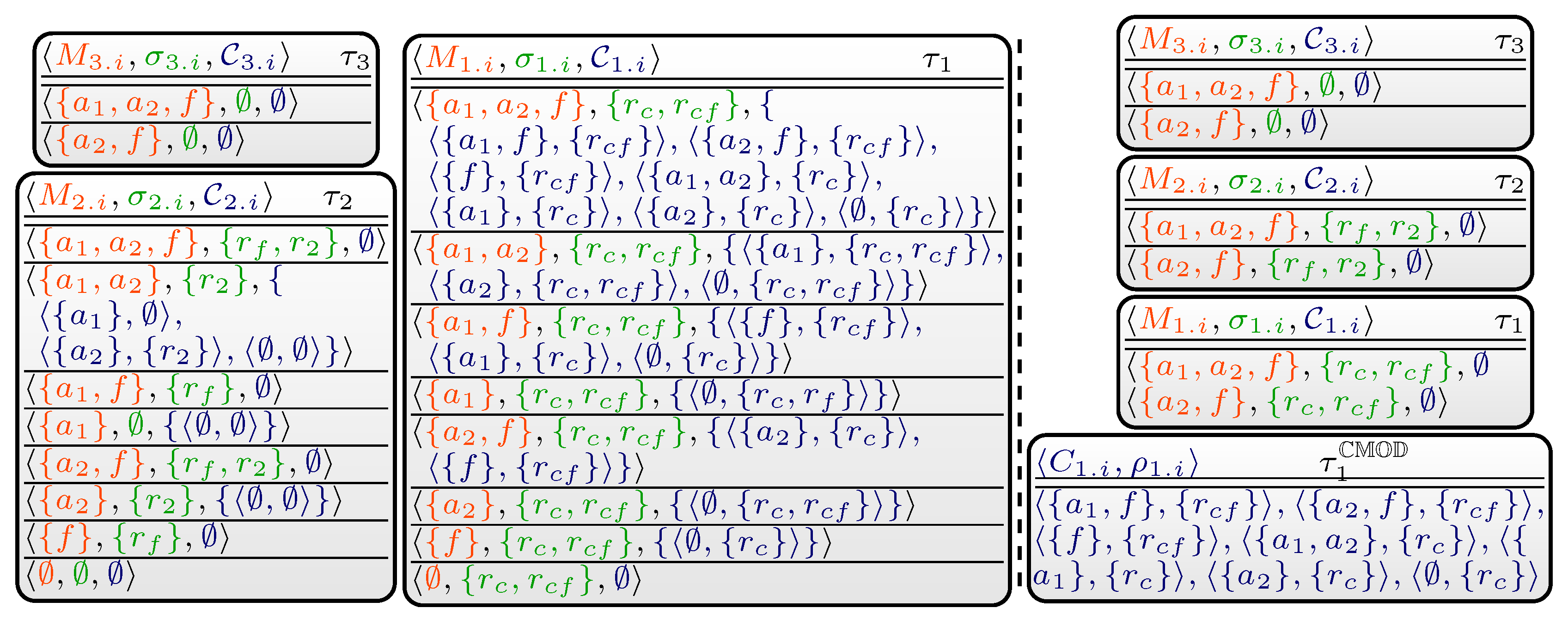
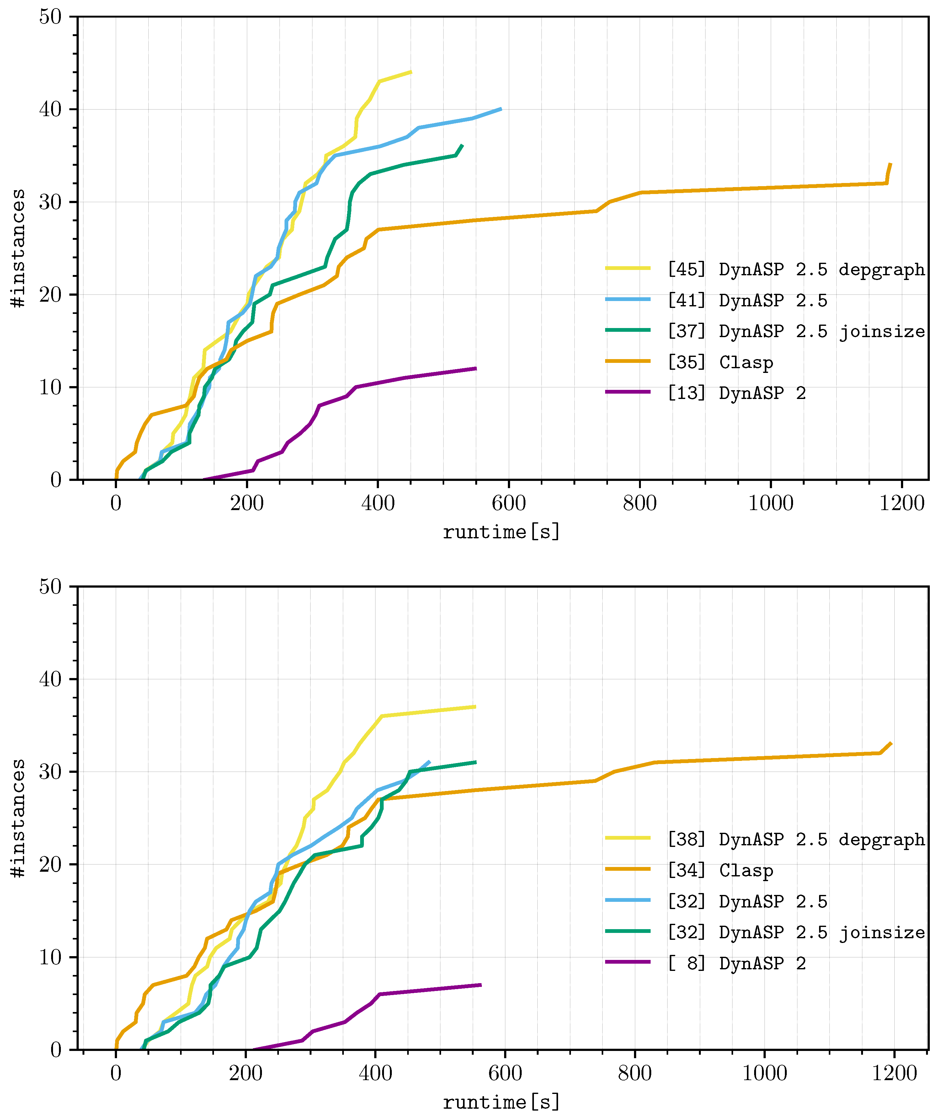
Table 1.
The table illustrates detailed benchmark results, where data for the best possible among all five runs is depicted (top) and results for the median run are shown (bottom). All columns illustrate values in seconds, except the first two columns. Column “Solver” indicates a solving system or configuration and “Solved” refers to the number of solved instances. Then, columns “TD”, “3.I”, “3.II”, and “3.III” list the total runtime in seconds over all solved instances for computation involving obtaining TDs, Pass 3.I, Pass 3.II, and Pass 3.III, respectively. Column “” refers to the total runtime in seconds over all solved instances. The last column depicts the PAR2 score over all instances, where timeouts are treated as two times the timeout (“PAR2 score”). Bold-face text indicates the best result in the corresponding column.
| Solver | Solved | Runtimes (Best) among Solved Instances | PAR2 Score | ||||
|---|---|---|---|---|---|---|---|
| TD | 3.I | 3.II | 3.III | ||||
| Clasp 3.3.0 | 35 | - | - | - | - | 11,493.98 | 93,093.98 |
| DynASP2 | 13 | 7.96 (0.2%) | - | - | - | 3978.29 | 138,378.29 |
| DynASP2.5 | 41 | 21.68 (0.2%) | 130.10 (1.4%) | 585.47 (6.2%) | 8656.48 (92.2%) | 9393.73 | 76,496.74 |
| “depgraph” | 45 | 408.72 (4.0%) | 138.21 (1.4%) | 595.58 (5.8%) | 9033.70 (88.8%) | 10,176.21 | 67,667.71 |
| “joinsize” | 37 | 22.82 (0.3%) | 120.19 (1.3%) | 544.18 (6.1%) | 8250.16 (92.3%) | 8937.35 | 85,654.00 |
| Solver | Solved | Runtimes (median) among solved instances | PAR2 Score | ||||
| TD | 3.I | 3.II | 3.III | ||||
| Clasp 3.3.0 | 34 | - | - | - | - | 11,688.58 | 94,523.53 |
| DynASP2 | 8 | 8.74 (0.2%) | - | - | - | 4370.83 | 149,289.20 |
| DynASP2.5 | 32 | 21.91 (0.2%) | 140.08 (1.3%) | 685.15 (6.4%) | 9878.67 (92.1%) | 10,725.81 | 96,405.37 |
| “depgraph” | 38 | 473.12 (4.1%) | 146.33 (1.3%) | 661.00 (5.8%) | 10,118.22 (88.8%) | 11,398.67 | 81,425.39 |
| “joinsize” | 32 | 25.47 (0.2%) | 129.41 (1.3%) | 596.62 (5.8%) | 9538.77 (92.7%) | 10,290.27 | 97,260.77 |
Publisher’s Note: MDPI stays neutral with regard to jurisdictional claims in published maps and institutional affiliations. |
© 2021 by the authors. Licensee MDPI, Basel, Switzerland. This article is an open access article distributed under the terms and conditions of the Creative Commons Attribution (CC BY) license (http://creativecommons.org/licenses/by/4.0/).
Share and Cite
MDPI and ACS Style
Fichte, J.K.; Hecher, M.; Morak, M.; Woltran, S. DynASP2.5: Dynamic Programming on Tree Decompositions in Action. Algorithms 2021, 14, 81. https://0-doi-org.brum.beds.ac.uk/10.3390/a14030081
AMA Style
Fichte JK, Hecher M, Morak M, Woltran S. DynASP2.5: Dynamic Programming on Tree Decompositions in Action. Algorithms. 2021; 14(3):81. https://0-doi-org.brum.beds.ac.uk/10.3390/a14030081
Chicago/Turabian StyleFichte, Johannes K., Markus Hecher, Michael Morak, and Stefan Woltran. 2021. "DynASP2.5: Dynamic Programming on Tree Decompositions in Action" Algorithms 14, no. 3: 81. https://0-doi-org.brum.beds.ac.uk/10.3390/a14030081
Note that from the first issue of 2016, this journal uses article numbers instead of page numbers. See further details here.