Article

Union and Intersection Operators for Thick Ellipsoid State Enclosures: Application to Bounded-Error Discrete-Time State Observer Design

ENSTA Bretagne, Lab-STICC, 29806 Brest, France
*
Author to whom correspondence should be addressed.
Submission received: 3 March 2021 / Revised: 9 March 2021 / Accepted: 11 March 2021 / Published: 14 March 2021
(This article belongs to the Special Issue Algorithms for Reliable Estimation, Identification and Control II)

Abstract

:
Thick ellipsoids were recently introduced by the authors to represent uncertainty in state variables of dynamic systems, not only in terms of guaranteed outer bounds but also in terms of an inner enclosure that belongs to the true solution set with certainty. Because previous work has focused on the definition and computationally efficient implementation of arithmetic operations and extensions of nonlinear standard functions, where all arguments are replaced by thick ellipsoids, this paper introduces novel operators for specifically evaluating quasi-linear system models with bounded parameters as well as for the union and intersection of thick ellipsoids. These techniques are combined in such a way that a discrete-time state observer can be designed in a predictor-corrector framework. Estimation results are presented for a combined observer-based estimation of state variables as well as disturbance forces and torques in the sense of an unknown input estimator for a hovercraft.

1. Introduction

Predictor-corrector approaches for the model-based estimation of state variables and disturbances were presented in several previous research activities [1,2]. These approaches rely on predicting state enclosures for sets of ordinary differential equations either in an interval-based form [3,4], perform Taylor series expansions with respect to time as well as uncertain parameters and initial conditions [5], or employ Taylor model-based approaches [6,7]. However, these techniques are not directly capable of representing inner and outer bounds of the estimated domain in a unified manner as they were determined by means of affine sets [8], combinations of affine arithmetic with automatic differentiation [9], and data-driven overapproximation techniques for a reachability analysis [10] in current references. On the one hand, the predictor-corrector methods mentioned above provide guaranteed outer bounds of all state variables that are consistent with the state equations as well as with measured output information. Both, state equations and output models, the latter representing sensor characteristics with bounded noise, may include interval parameters to reflect limited knowledge and the influence of model simplifications. On the other hand, however, the lack of information concerning domains that belong to the exact sets of reachable states makes it impossible to distinguish between the phenomena of wide state enclosures as a consequence of uncertainty or the result of wide bounds due to pessimism in numerical evaluations. The latter aspect is well-known in the frame of interval analysis and denoted as overestimation that can be traced back to the so-called dependency effect (numerous variables are treated as independent despite underlying physical or mathematical correlations) or to the wrapping effect (complex-shaped solution sets are replaced conservatively by more simple outer bounds which are subsequently propagated further) [11,12,13,14].
From this description, it becomes obvious that it is desirable to express uncertainty on the bounds of the domains of reachable states in the frame of simulation and state estimation techniques. Recently, corresponding set representations were developed which allow to express either a notion of variables certainly belonging to a solution set or certainly not belonging to the set (denoted as a relative distance measure interval arithmetic [15]); alternatively, the notion of thick intervals, thick boxes, thick functions, and thick ellipsoids can be seen as an approach to handle this kind of uncertainty on set boundaries [16]. Moreover, combinations of fuzzy and interval methods as those presented in [17] represent other currently investigated techniques that aim at expressing uncertainty on state boundaries.
Especially the use of ellipsoids as enclosures for reachable sets [18,19] is a promising approach because such domains naturally arise as descriptions of provable stability domains for nonlinear dynamic systems if the corresponding analysis is performed with the help of quadratic Lyapunov functions. Moreover, propagating ellipsoids over a dynamic system model with sufficient smoothness properties typically leads again to a solution set with boundaries that can effectively be described by enclosing ellipsoids if the domains of interest are sufficiently small. For a proof of this property, see [20], where it has been shown that the Hausdorff distance between the true solution and the ellipsoidal enclosure reduces at least linearly for decreasing domain sizes.
Computations of ellipsoidal enclosures inherently have the property of a constant complexity if they are applied recursively. In addition, their enclosure quality enhances automatically for reducing domain sizes which is in contrast to the propagation of polytopic and zonotopic domains [21,22]. There, the number of vertices of the solution sets—especially after intersecting the results of measurement-based innovation steps with the outcome of state prediction stages—tends to increase in each time step. This leads to the necessity to employ specific techniques to reduce the complexity at least after a certain number of evaluation steps [23]. Although these polytopic and zonotopic techniques help to reduce overestimation, a constant complexity over subsequent time steps for the evaluation of dynamic systems can typically only be observed if the solutions are restricted to domains with a fixed number of vertices such as axis-aligned intervals or parallelepipeds as a special kind of preconditioned interval boxes after a linear change of coordinates.
Previous work of the authors has focused on the development of thick ellipsoid function evaluations [20] and recursive simulation approaches [24], where the inner bounds represent the domains of certainly reachable states and the outer bounds reflect the worst-case uncertainty. So far, only extensions of sufficiently smooth function evaluations (the basic arithmetic operations of addition, subtraction, multiplication and division) as well as the evaluation of nonlinear standard functions (such as trigonometric or exponential functions) were investigated. In order to implement state estimation schemes, it is further necessary to define outer and inner solution enclosures in ellipsoidal form for union and intersection operators. These operators are investigated in more detail in this paper so that they form the basis for the implementation of a discrete-time state estimation procedure. The estimator’s structure resembles the one of a discrete-time Kalman filter [25] or of suitable generalizations for nonlinear systems [26,27,28,29], where a state prediction stage is employed to forecast future reachable states and this a-priori knowledge is subsequently refined in an innovation (i.e., correction) stage as soon as measured data become available.
In Section 2 of this paper, a review of thick ellipsoids as a representation of uncertain state domains for dynamic systems is given. Based on their introduction, inner and outer union as well as intersection operators are derived and summarized in Section 3 which form the basis for state estimation in the frame of (quasi-)linear discrete-time system models. The corresponding novel, thick ellipsoid state estimation procedure is derived in Section 4 before a representative benchmark scenario for state and disturbance estimation of a hovercraft model is discussed in Section 5. Finally, this article is concluded by an outlook on future work in Section 6.

2. Thick Ellipsoids

Thick ellipsoids were introduced by the authors in [20,24] to represent conservative outer bounds of the domains of reachable states of dynamic systems in parallel with inner bounds which represent those states that belong to the reachable solutions with absolute certainty. Geometrically, a thick ellipsoid can be understood as an ellipsoid with an uncertain boundary as illustrated in the left-hand side of Figure 1 that allows for enclosing a complexly shaped domain A k according to
E k I A k E k O .
The previous publications [20,24] focused on propagating this ellipsoidal domain via a nonlinear map
x k + 1 = f x k
so that the true outputs A k + 1 after performing a state prediction according to (2) are again enclosed by a thick ellipsoid in a computationally cheap manner. For that reason, linear matrix inequalities are only employed in offline phases for the derivation of the proposed solution technique. Our procedure avoids the search for the globally optimal (i.e., tightest possible) solution of state prediction (and also the subsequent innovation stages) by a replacement of the online use of linear matrix inequalities or complex minmax optimization tasks by low-dimensional optimizations. Classically, the task of finding ellipsoidal state enclosures would be solved by using the aforementioned, often time-consuming techniques in each time step if the approaches published in [19,30,31,32] were applied directly. However, for the goal of a reduction of the computational effort and, hence, for a simplification of real-time implementability, we propose low-dimensional optimization procedures which avoid the search for the typically large number of degrees of freedom if the optimal inner and outer ellipsoids E k I and E k O , respectively, were computed.
In the following, we recapitulate the mathematical definitions of thick ellipsoids together with binary operators and function extensions. Note, similar concepts were also introduced in [16] for so-called thick intervals (which represent scalar interval variables with uncertain lower and upper bounds) as well as thick boxes as the Cartesian product of thick intervals. A closely related concept is the so-called type-2 interval arithmetic discussed in detail in [15].
Definition 1
(Thick ellipsoid). Define a thick ellipsoid E = E μ , Γ , ρ ¯ ; ρ ¯ as a subset of the power set P R n so that
E = A P R n | E I A E O
with
E I = x R n | x μ T ρ ¯ Γ T ρ ¯ Γ 1 x μ 1 , E O = x R n | x μ T ρ ¯ Γ T ρ ¯ Γ 1 x μ 1
and 0 ρ ¯ ρ ¯ .
Definition 2.
(Thick ellipsoid binary operators and function extensions). A thick ellipsoid extension of the binary operators { + , , · , / , , } (For the case of division, the value zero is assumed not to belong to the denominator expression in analogy to classical interval arithmetic [11]) satisfies the relation
A A B B C = A B C A B .
The quantity C = A B is also a thick ellipsoid, which is typically neither minimal with respect to its width nor uniquely defined. Analogously, f is a thick ellipsoid function extension of f : R n R m , if
A A B = f A B B = f A .
For the implementation of algorithms that allow for evaluating nonlinear mapping functions (2) with the help of thick ellipsoids, the reader is referred to [20,24]. In this paper, we impose a specific, (quasi-)linear structure of the considered system models, so that the thick ellipsoid function evaluation can be simplified by a newly derived simulation scheme according to Section 3.1.

3. Union and Intersection of Thick Ellipsoid Enclosures

Parameter-dependent quasi-linear system models in the form
x k + 1 = A x k , p k · x k
with p k p ¯ k ; p ¯ k , where p ¯ j , k p j , k p ¯ j , k , j { 1 , , m } , are a special case of the nonlinear system representation introduced in (2).
In many cases, they arise if discrete-time state equations (2) with an equilibrium state at x k + 1 = x k = 0 are re-written by means of symbolic formula manipulation in which the dependence on the state vector x k is factored out from the system model (2). In such cases, it needs to be ensured that all entries of A x k , p k are well-defined because they do not contain any singularities after factoring out the state vector x k and are, therefore, finite for the complete operating domain of interest. In addition, these models arise if centered-form representations of nonlinear system models are computed either by determining interval extensions of the system’s Jacobian or by means of techniques for slope arithmetic. For details concerning these latter two options, the reader is referred to [33,34,35].

3.1. Mapping of Thick Ellipsoidal Domains via (Quasi-)Linear System Models

In general, the evaluation of system models in the form (7) is possible with the help of the general solution approach presented in [20,24] if an augmented state vector is introduced that contains not only the actual state variables x k but also the parameter vector p k in terms of discretized integrator disturbance models for which p k + 1 = p k holds. However, the examples investigated in [24] have shown that doing so leads to conservativeness of the solutions. The reason for this observation is that the parameters p k become correlated with the state vector x k so that their outer bounds start to expand despite the aforementioned assumption of uncertain but temporally constant values. Hence, the methods summarized in this subsection (together with the intersection operators included in the state estimator according to Section 4) resolve the corresponding issue by introducing uncertain parameters as entries in the system matrix. When doing so, their enclosures may even be reset at each sampling instant k to new interval bounds. As shown subsequently, this option allows for analogously dealing with (outer) state bounds influencing the dynamics matrix A x k , p k .
For the sake of compactness, the short-hand notation A k = A x k , p k A k is used in the following to denote an interval matrix containing the worst-case outer range bounds of all matrix entries at a specific time instant k.

3.1.1. Outer Bounds

Given an ellipsoid
E k = x k R n | x k T · Q k 1 · x k 1
that is described by a positive definite shape matrix Q k = Q k T > 0 and centered at the origin x k = 0 of the state space, it is desired to enclose the exact (generally non-ellipsoidal) solution set of the mapping (7) in terms of a guaranteed outer ellipsoidal bound
E k + 1 O = x k + 1 R n | 1 α O , k + 1 2 · x k + 1 T · Q k + 1 1 · x k + 1 1
with degrees of freedom concerning the choice of the shape matrix Q k + 1 and its stretch parameter α O , k + 1 > 0 . The latter will be computed by means of a simple line-search optimization procedure to avoid the necessity for an online solution of linear matrix inequalities.
With the help of the free matrix variable R k , the shape matrix of the predicted ellipsoid is described by
Q k + 1 = Q k + 1 T = A ˜ k · R k · A ˜ k T > 0 , R k = R k T > 0 ,
where A ˜ k is some invertible point matrix typically satisfying
A ˜ k A k .
This definition is inherited from the propagation of a representative point in the interior of E k which was chosen to be its midpoint in [20,24].
Remark 1.
Possible choices for the parameterization of the matrices R k and A ˜ k introduced in (10) and (11) are discussed in the illustrating example in Section 3.1.3.
Assuming regularity of A x k , p k · Q k · A T x k , p k for all x k E k , p k p k , the exact solution of the mapping (7) is defined by
E k + 1 * = { x k + 1 R n | x k + 1 T · A k · Q k · A k T 1 · x k + 1 1 , where A k = A x k , p k with x k E k , p k p k } ,
where E k + 1 * E k + 1 O needs to be satisfied for (9) to represent a guaranteed outer bound of the solution domain. Note, even if this regularity assumption does not hold, the following Theorem 1 remains true.
Theorem 1
(Guaranteed outer bound). The ellipsoid E k + 1 O according to Equation (9) is a guaranteed outer bound for E k + 1 * if the matrix inequality
M k + 1 : = Q k 1 A T x k , p k · A ˜ k T A ˜ k 1 · A x k , p k α O , k + 1 2 R k 0
holds for all x k E k and p k p k .
Proof. 
Without any assumptions on the regularity of A x k , p k · Q k · A T x k , p k , the relation E k + 1 * E k + 1 O is satisfied, if mapping the domain E k + 1 O one time step back leads to a domain S k that is a superset of the ellipsoid E k according to S k E k with
S k = { x k R n | x k T · A T x k , p k · 1 α O , k + 1 2 · A ˜ k · R k · A ˜ k T 1 · A x k , p k · x k 1 , where x k E k , p k p k } .
Geometrically speaking, this means that the level curve of height 1 of the quadratic form in (8), which corresponds to the bound of the ellipsoid E k , must be an inner bound for the level curve of identical height of S k . This condition corresponds to the scalar inequality
x k T · A T x k , p k · 1 α O , k + 1 2 · A ˜ k · R k · A ˜ k T 1 · A x k , p k · x k x k T · Q k 1 · x k
for all x k E k and p k p k .
Factoring out the vector x k to the left and right of (15) turns this scalar inequality into the matrix inequality
A T x k , p k · 1 α O , k + 1 2 · A ˜ k · R k · A ˜ k T 1 · A x k , p k Q k 1 0 ,
which (for the choice of a regular matrix A ˜ k ) is equivalent to the condition
A T x k , p k · A ˜ k T · α O , k + 1 2 R k 1 · A ˜ k 1 · A x k , p k Q k 1 0 .
Removing the difference of the two matrices in (17) with the help of the Schur complement formula [36,37] leads to Equation (13) which completes the proof of Theorem 1. □
Remark 2.
As stated before, the quasi-linear system matrix A x k , p k is bounded by an element-wise defined interval matrix A x k , p k A k = A ¯ k ; A ¯ k . Therefore, a conservative solution to the matrix inequality in Theorem 1 can be determined by searching for a state- and parameter-independent, strictly positive definite matrix α O , k + 1 2 R k that satisfies the interval-valued matrix inequality
M k + 1 M k + 1 = Q k 1 A k T · A ˜ k T A ˜ k 1 · A k α O , k + 1 2 R k 0 .
This matrix inequality can be cast into a linear one by the substitution
P k + 1 O = P k + 1 O T = α O , k + 1 2 R k > 0
to make standard routines for linear matrix inequalities such as theMatlabtoolboxSeDuMiin combination withYalmip[38,39] applicable if (18) is further replaced by the convex combination of a finite number of extremal realizations with the help of the ideas given in [40,41]. The extremal realizations can be obtained by computing an interval extension of the state- and parameter-dependent system matrix A x k , p k with the help of toolboxes such asIntLab[42] forMatlaband determining all matrix entries that have a non-zero diameter. Then, it is possible to represent (18) by the convex polytope
D = M k + 1 | M k + 1 ( ξ ) = v = 1 n v ξ v · M v , k + 1 ; v = 1 n v ξ v = 1 ; ξ v 0 ,
which is only used in the following example for the sake of comparison with the proposed method, where for the list of all n v = 2 n 2 interval vertices formed of A ¯ k and A ¯ k the corresponding extremal realizations
M v , k + 1 = Q k 1 A v , k T · A ˜ k T A ˜ k 1 · A v , k P k + 1 O , v { 1 , , n v } ,
are defined and need to be negative semi-definite with M v , k + 1 0 . Note, this formulation of all (21) directly accounts for the structural symmetry of (18). A (nearly) optimal solution can be obtained by minimizing trace P k + 1 O , cf. [43,44], which can be employed as a substitute for the optimization task involving the logarithm of the shape matrix determinant according to ([45], Appendix C).
To avoid the necessity to solve linear matrix inequalities in each temporal discretization step of a dynamic system, the following Theorem 2 describes a relaxed version of the solution procedure after a-priori fixing the matrix R k , for example, by setting R k = Q k .
Theorem 2
(Eigenvalue criterion for outer ellipsoidal bounds). For a fixed combination of the shape and stretch parameters R k and α O , k + 1 , respectively, E k + 1 O is a guaranteed outer enclosure of the solution set E k + 1 * , if
λ i mid M k + 1 + ρ rad M k + 1 0
holds for all i { 1 , , 2 n } , where λ i mid M k + 1 is the i-th eigenvalue of 1 2 · M ¯ k + 1 + M ¯ k + 1 and ρ rad M k + 1 the spectral radius of 1 2 · M ¯ k + 1 M ¯ k + 1 .
Proof. 
Due to the structural symmetry of M k + 1 , all possible eigenvalues λ i M k + 1 of M k + 1 M k + 1 are guaranteed to be real-valued. According to Rohn [46,47], interval bounds for the range of each eigenvalue are given by the enclosures
λ i M k + 1 λ i , M = λ i mid M k + 1 + 1 ; 1 · ρ rad M k + 1
located on the real axis of the complex plane. If sup λ i , M 0 holds for all i { 1 , , 2 n } , Theorem 1 is satisfied due to the negative semi-definiteness of the interval matrix (18). □
Remark 3.
To enhance the efficiency of the enclosure technique, the eigenvalue bounds from (23) can be combined with the upper eigenvalue bound λ max , M obtained from the Gershgorin circle criterion [48]
λ max , M max i { 1 , , 2 n } sup M i , i + j = 1 , j i 2 n M i , j .
If this is not efficient, all vertices of the interval matrix (18) could be tested for negative semi-definiteness.
Remark 4.
The optimal, i.e., smallest volume ellipsoid after fixing the matrix R k , for example, by the choice R k = Q k , is obtained with the help of Theorem 2 if the parameter α O , k + 1 > 0 is minimized by a line search procedure so that (22) remains satisfied. For α O , k + 1 , the outer bound becomes infinitely large.

3.1.2. Inner Bounds

Inner ellipsoidal bounds
E k + 1 I = x k + 1 R n | 1 α I , k + 1 2 · x k + 1 T · Q k + 1 1 · x k + 1 1
with the shape matrix defined in (10) describe domains that are guaranteed to belong to the solution set according to E k + 1 I E k + 1 * are characterized by the following Theorem 3.
Theorem 3
(Guaranteed inner bound). The ellipsoid E k + 1 I according to Equation (25) is a guaranteed outer bound for E k + 1 * if the matrix inequality
N k + 1 : = α I , k + 1 2 · R k 1 A ˜ k 1 · A x k , p k T A ˜ k 1 · A x k , p k 1 Q k 0
holds for all x k E k and p k p k .
Proof. 
The proof of Theorem 3 follows a similar reasoning as the proof of Theorem 1. If the matrix A x k , p k · Q k · A T x k , p k has full rank for all x k E k and p k p k , E k + 1 I E k + 1 * holds, if the level curve of height 1 of the quadratic form in (25), which corresponds to the bound of the ellipsoid E k + 1 I , is fully contained in the interior of E k + 1 * according to the scalar inequality
x k + 1 T · 1 α I , k + 1 2 · A ˜ k · R k · A ˜ k T 1 · x k + 1 x k + 1 T · A x k , p k · Q k · A T x k , p k 1 · x k + 1
This condition corresponds to the matrix inequality
1 α I , k + 1 2 · A ˜ k · R k · A ˜ k T 1 A x k , p k · Q k · A T x k , p k 1 0 ,
which is equivalent to
1 α I , k + 1 2 · R k 1 A ˜ k T · A T x k , p k · Q k 1 · A 1 x k , p k · A ˜ k 0
under the above-mentioned regularity assumption.
Removing the difference of matrices in (29) by the application of the Schur complement formula completes the proof of Theorem 3. □
Remark 5.
In analogy to Equation (18), a conservative formulation of Theorem 3 can be given by the interval-valued matrix inequality
N k + 1 N k + 1 = α I , k + 1 2 · R k 1 A ˜ k 1 · A k T A ˜ k 1 · A k 1 Q k 0
for which a common solution after the linearizing variable substitution
P k + 1 I = P k + 1 I T = α I , k + 1 2 · R k 1 > 0
needs to be found. An optimization of this solution is possible by a minimization of trace P k + 1 I , (replacing the optimization task involving the logarithm of the shape matrix determinant according to [45] Appendix C), where for a polytopic representation of the domain N k + 1 according to (21) the entry-wise defined vertices of the matrix inverse A ˜ k 1 · A k 1 need to be found. A relaxation into a computationally less expensive eigenvalue test is given by Theorem 4.
Theorem 4
(Eigenvalue criterion for inner ellipsoidal bounds). For a fixed combination of the shape and stretch parameters R k and α I , k + 1 , respectively, E k + 1 I is a guaranteed inner enclosure of the solution set E k + 1 * , if
λ i mid N k + 1 + ρ rad N k + 1 0
holds for all i { 1 , , 2 n } , where the mid and rad operators are defined as in Theorem 2.
Proof. 
The proof of Theorem 4 results from a direct application of the proof of Theorem 2 after exchanging the sign condition of the respective inequalities, where inf λ i , N 0 needs to hold for all i { 1 , , 2 n } . □
Remark 6.
To enhance the efficiency of the enclosure technique, the eigenvalue bounds from (32) can be combined with the lower eigenvalue bound λ min , N obtained from the Gershgorin circle criterion
λ min , N min i { 1 , , 2 n } inf N i , i j = 1 , j i 2 n N i , j .
If this is not efficient, all vertices of the interval matrix (30) could be tested for positive semi-definiteness. However, this is only recommended for sufficiently small values of n.
Remark 7.
The optimal, i.e., largest volume ellipsoid after fixing the matrix R k , for example, by the choice R k = Q k , is obtained with the help of Theorem 4 if the parameter α O , k + 1 > 0 is maximized by a line search procedure so that (32) remains satisfied. For α I , k + 1 = 0 or non-regular matrices A ˜ k 1 · A k , the inner ellipsoidal bound is the empty set.
Using identical matrices R k for the outer and inner ellipsoids, the thick ellipsoid sets is defined by
E k + 1 = E k + 1 0 , R k 1 2 · A ˜ k , α I , k + 1 ; α O , k + 1 .

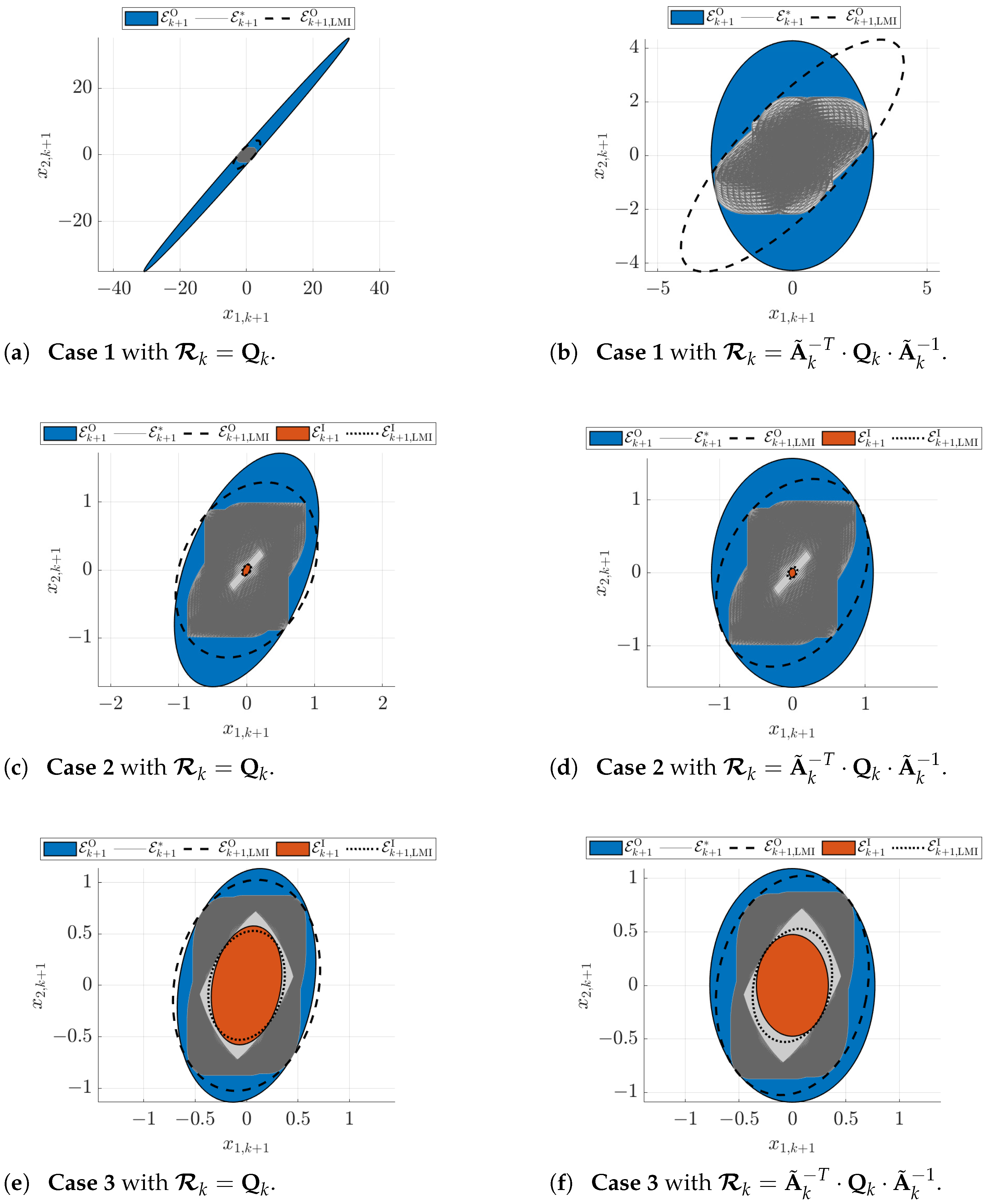
3.1.3. Illustrating Example

As an illustrating example, consider the system model
x k + 1 = 0.5 p 1 p 2 0.6 · x k
with the independent parameters p 1 and p 2 , where
x k E k with Q k = 1 0 0 2 .
To show the influence of parameter uncertainty on the computed ellipsoidal enclosures, the following cases are distinguished in Figure 2:
case 1
p 1 1 ; 2 , p 2 1 ; 2 ;
case 2
p 1 0.25 ; 0.5 , p 2 0.25 ; 0.5 ;
case 3
p 1 0.1 ; 0.2 , p 2 0.1 ; 0.2 .
In the left column of Figure 2, the parameter matrix R k = Q k is chosen, while it is set to R k = A ˜ k T · Q k · A ˜ k 1 in the right column, where A ˜ k is the interval midpoint of the uncertain system matrix.
Obviously, for the smaller uncertainty in the cases 2 and 3, the first setting is superior. This is not astonishing because it corresponds to that choice of matrix that would be employed for the covariance prediction in an Extended Kalman Filter (EKF). As it is well known, strong deviations from a point-valued system matrix A k may turn an EKF quite inaccurate. Then, other choices of the forecasted covariance are often superior, as they could be determined by the Unscented Kalman Filter technique [27]. This approach was not investigated here. However, the almost symmetric interval bounds of A k motivate the second choice of R k , which corresponds to Q k + 1 = Q k .
Moreover, it should be pointed out that the case 1 in Figure 2a,b corresponds to a scenario in which the inner bound is empty, the case 2 in Figure 2c,d to a scenario in which the inner bound just appears due to the matrix A k containing purely regular realizations; finally, Figure 2e,f shows the case of small uncertainty with a clearly visible inner solution set, where the proposed one-parameter optimization task from the previous subsections provides results that are close to the solution of the robust linear matrix inequality design, where R k is not predefined but rather optimized with the help of the matrices P k + 1 O and P k + 1 I to obtain independent outer and inner enclosures (dashed and dotted lines, respectively).

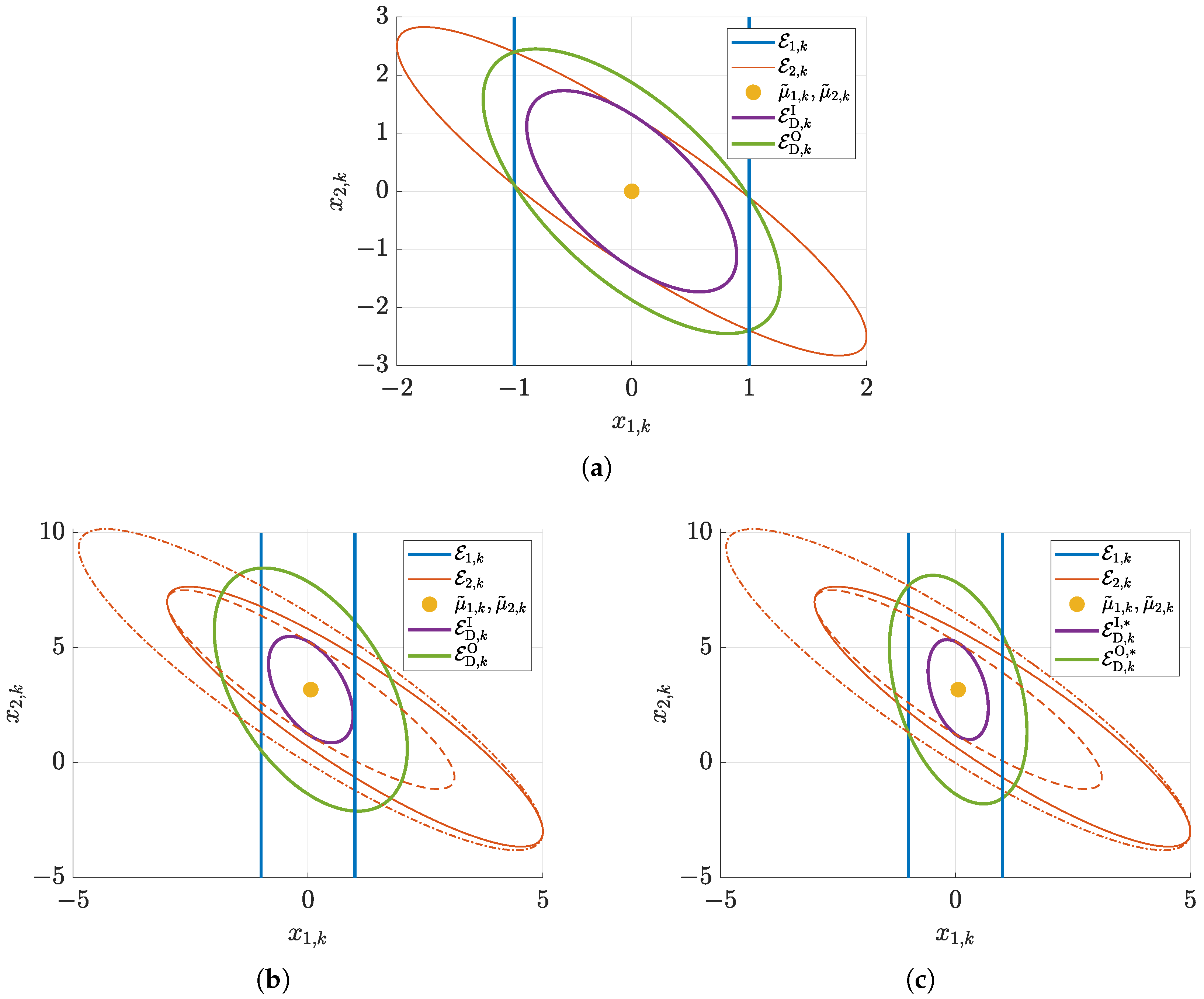
3.2. Dikin Ellipsoids for the Intersection of Ellipsoids

The intersection of two ellipsoidal (state) domains is a fundamental operation for the estimation of state variables in a bounded-error framework. For that reason, this section introduces corresponding procedures that are readily applicable to thick ellipsoids, starting with the well-known case of two ellipsoids with identical midpoints. These results are further generalized to the case, where the ellipsoid midpoints may be different from each other.

3.2.1. Intersection of Ellipsoids with Identical Midpoints

Outer as well as inner ellipsoidal representations for the intersection of various ellipsoidal domains were investigated in numerous publications. Especially, the reference [49] gives a thorough overview of a large number of applicable techniques that can be cast into computationally feasible optimization problems. Basically, all of these routines are based on the use of linear matrix inequalities. At each intersection stage, such linear matrix inequalities need to be solved when computing so-called inner and outer bounds by means of a technique that is based on findings of Löwner and John [50]. Analogously, this holds for the Nerimovski approximation [51] that is compared with the first option in [49].
To avoid the necessity for solving linear matrix inequalities explicitly during online applications (note, these matrix inequalities are exploited for the offline proof of the validity of the following enclosure relations), a conservative approximation based on the so-called Dikin ellipsoids [49] is considered in this paper. These ellipsoids can be applied to describe inner and outer bounds for the intersection I k of m ellipsoids
E i , k = x k R n | x k T · Q i , k 1 · x k 1 , i { 1 , , m }
with an identical center located in the origin of the state space. The following relations for the shape matrices hold equally for identical non-zero center points.
Using the results of Lemma 5 in [49], the inner and outer bounds are given by
E D , I , k I k E D , O , k
with E D , I , k = E D , k 2 and E D , O , k = E D , k 2 m , respectively, where
E D , k r = x k R n | x k T · r 1 · Q D , k 1 · x k 1
is defined for the common shape matrix
Q D , k 1 = 2 i = 1 m Q i , k 1 .
This definition of inner and outer ellipsoidal enclosures corresponds to a thick ellipsoid introduced in the Definitions 1 and 2 in the form
E D , k = E D , k 0 , Γ D , k , 2 ; 2 m with Γ D , k = Q D , k 1 2 .
Although these enclosures are generally suboptimal, we restrict ourselves to these Dikin ellipsoids due to their computational inexpensive evaluation which is advantageous if real-time state estimation procedures are desired. A generalization to the case of ellipsoids with different midpoints is presented in the following subsection.
Efficient techniques that allow for checking whether the intersection of two ellipsoids is empty were published in [52,53]. This check is especially interesting if the thick ellipsoid state observer technique derived in the following section is applied to tasks in the area of fault detection. There, the case that a predicted state domain does not intersect with those domains that are compatible with sensor data typically indicates failures of system components, actuators, or sensors. This corresponds to the fact that the investigated (nominal) system model is proven to be infeasible.
A further related technique, however, not only relying on ellipsoidal state enclosures was very recently derived in [54]. There, outer bounds for the domains of reachable states are characterized by ellipsoids, while disturbances are bounded by zonotopes that may become degenerate if one or more coordinates are unbounded. This property of degeneracy will be picked up again in Section 3.2.3, where an example is presented in which only partial state measurements are available in the thick ellipsoid framework.

3.2.2. Generalization to the Intersection of Ellipsoids with Different Midpoints

An extension of the technique for computing Dikin ellipsoids to a scenario in which two ellipsoids with different centers are intersected, is based on the following three-stage procedure:
Step 1
Determine the common center point for the desired inner and outer bounds of the intersection that must be included in all ellipsoids to be intersected;
Step 2
Determine initial approximations of the shape matrices for the inner and outer bounds according to Section 3.2.1;
Step 3
For non-empty inner bounds, correct the outer enclosure so that the inner and outer ellipsoid surfaces become parallel to each other and, thus, form a thick ellipsoid E .
Step 3*
As an alternative to Step 3, the initial outer enclosure remains fixed and the inner ellipsoid surface is adapted to become parallel to each other to form a thick ellipsoid E .
As a heuristic approach for the computation of the common center point μ ˜ k in Step 1 of two ellipsoids that are described by the midpoints μ 1 , k and μ 2 , k as well as the shape matrices Q 1 , k and Q 2 , k , respectively, the first one is interpreted as the prior knowledge in the innovation step of a Kalman filter [25,55] and the second one as the corresponding information of the state measurement.
Under this assumption, one obtains the Kalman gain matrix
L k = Q 1 , k · Q 1 , k + Q 2 , k 1
with the updated ellipsoid midpoint
μ ˜ k = μ 1 , k + L k · μ 2 , k μ 1 , k
that is now used for the solution of the Steps 2 and 3 listed above.
For both ellipsoids i { 1 , 2 } to be intersected, scaling factors ξ i > and ζ i > are determined which represent the minimum and maximum distances of the new midpoint from the ellipsoid surface according to
ξ i , k = 1 Δ μ i , k and ζ i = 1 + Δ μ i , k ,
with
Δ μ i , k = Q i , k 1 2 · μ ˜ k μ i , k
and Δ μ i , k as the Euclidean norm of the vector-valued argument.
In such a way, both ellipsoids to be intersected can be enclosed by thick ellipsoids
E i , k = E i , k μ ˜ k , Γ ˜ i , k , ξ i , k ; ζ i , k with Γ ˜ i , k = Q i , k 1 2 .
The initial inner approximation of the shape matrix of the resulting intersection is given by
Q k I = 2 · 2 · ξ 1 , k 2 · Q 1 , k 1 + ξ 2 , k 2 · Q 2 , k 1 1
according to the previous subsection, while its outer counterpart results in
Q k O = 4 · 2 · ζ 1 , k 2 · Q 1 , k 1 + ζ 2 , k 2 · Q 2 , k 1 1 .
Usually, these two shape matrices are not proportional to each other in an element-wise sense. Hence, the inner shape matrix Q k I is inflated in Step 3 according to the following theorem so that it contains the outer ellipsoid with certainty.
Theorem 5
(Thick interval representation of the Dikin intersection of ellipsoids with different midpoints). The thick Dikin ellipsoid
E D , k = E D , k μ ˜ k , Γ D , k , 1 ; min i { 1 , , n } λ i Q k O 1 · Q k I 1 2 w i t h Γ D , k = Q k I 1 2 .
represents guaranteed inner and outer bounds of the intersection of two ellipsoids with different midpoints if all parameters are chosen according to Equations (42)–(48).
Proof. 
The validity of the inner bound is a direct consequence of Lemma 5 in [49], and the construction of the matrix (45) as a guaranteed underapproximation of the domains to be intersected. The outer bound of (49) is represented by the shape matrix
Q k O = α O , k + 1 2 · Q k I .
It results from Equation (16) after setting A k = I , A ˜ k = I , Q k = Q k O , and R k = Q k I which yields
α O , k + 1 2 · I Q k O 1 · Q k I .
This inequality is satisfied if
α O , k + 1 2 min i { 1 , , n } λ i Q k O 1 · Q k I ,
where the expression in curly brackets denotes the minimum eigenvalue of the corresponding matrix product. Taking the square root of the inverse of this expression completes the proof of Theorem 5. □
The alternative solution according to Step 3* is given by the thick ellipsoid enclosure
E D , k * = E D , k * μ ˜ k , Γ D , k * , max i { 1 , , n } λ i Q k I 1 · Q k O 1 2 ; 1 with Γ D , k * = Q k O 1 2 ,
which is a direct consequence of Theorem 5 by searching for an ellipsoid parallel to the outer bound that is guaranteed to belong to the interior of the one with the shape matrix Q k I .
Remark 8.
Due to the fact that the relation
max i { 1 , , n } λ i Q k I 1 · Q k O = min i { 1 , , n } λ i Q k O 1 · Q k I 1 > 0
holds for arbitrary positive definite matrices Q k I and Q k O , the ratio between the volumes of the outer and inner ellipsoids in Equations (49) and (53) is identical. Hence, the variant (49) is typically preferred if thick ellipsoids with maximum volume inner enclosures are desired, while (53) provides tighter outer bounds.
Remark 9.
For ellipsoids with identical midpoints μ ˜ k = μ 1 , k = μ 2 , k , the ellipsoid of Theorem 5 is identical to the one in (41) if the midpoint parameter μ ˜ k is used instead of the value 0 in (41).

3.2.3. Illustrating Example

In this subsection, various examples for the intersection of ellipsoids and the result interpretation by means of the thick ellipsoids E D , k and E D , k * , respectively, are summarized. Figure 3a deals with the application of the intersection procedure of Section 3.2.1 for two ellipsoids identically centered at the origin with the shape matrices
Q 1 , k = 1 0 0 8 and Q 2 , k = 4 5 5 8 .
Here, both enclosures E D , k and E D , k * are identical. Moreover, the fact that the ellipsoid midpoints are identical results in inner and outer enclosures E D , k I and E D , k O that are quite close to the optimal ellipsoidal result representation.
To visualize the procedure of Section 3.2.2 for the case of two different midpoints
μ 1 , k = 0 0 T and μ 2 , k = 1 2 T
either with the shape matrices (55) or with the new shape matrices
Q 1 , k = 1 0 0 8 and Q 2 , k = 4 · 4 5 5 8 ,
the results in Figure 3c,d are presented. These results confirm the observation described in Remark 8 that the use of Equation (49) leads to tighter inner bounds, while Equation (53) possesses the better outer bounds. Depending on the application to detect states belonging to the solution set with certainty or proving in a guaranteed way that specific state domains are not reachable in the frame of a safety or feasibility test, either the first or the second option should be preferred.
However, the observed larger distance between the resulting inner and outer bounds in comparison with Figure 3a gives rise to the assumption that further improvements of the solution could be possible. This could either be done by means of the procedures in [49] or by intersecting the newly obtained outer bounds of both E D , k and E D , k * . Note, also the choice of the common ellipsoid midpoint represents a degree of freedom that can be investigated in future work together with possibilities to intersect the enlarged dashed-dotted bounds (which correspond to the outer ellipsoid surfaces of (46)) in a recursive manner with both E D , k and E D , k * .
Interestingly, the proposed intersection procedures can also be applied to the case where one of the original ellipsoids becomes degenerate. In practice, this is the case for a pure measurement of a single state variable. This case is considered in Figure 4, where in all subplots the matrices Q 1 , k from Equations (55) and (57) were replaced with Q 1 , k 1 = 1 0 0 0 , corresponding to x 1 , k 1 .
Due to the fact that the basic Formula (40) for computing Dikin ellipsoids only makes use of the inverted shape matrices, the solution procedure remains applicable for the degenerate case. This is a crucial requirement to use this intersection approach in cases in which only a subset to the state variables appears in the system’s output equation when considering state estimation procedures according to the following two sections. In Figure 4b,c, the new ellipsoid midpoint μ ˜ k results from the following adapted Kalman gain
L k = Q 2 , k · 1 0 · 1 0 · Q 2 , k · 1 0 + σ 1 , k 2 1 , where Q 1 , k 1 = σ 1 , k 2 0 0 0
with the updated ellipsoid midpoint
μ ˜ k = μ 2 , k + L k · 1 0 · μ 1 , k μ 2 , k ,
for which all remaining parameter values are defined in (56) and (57).

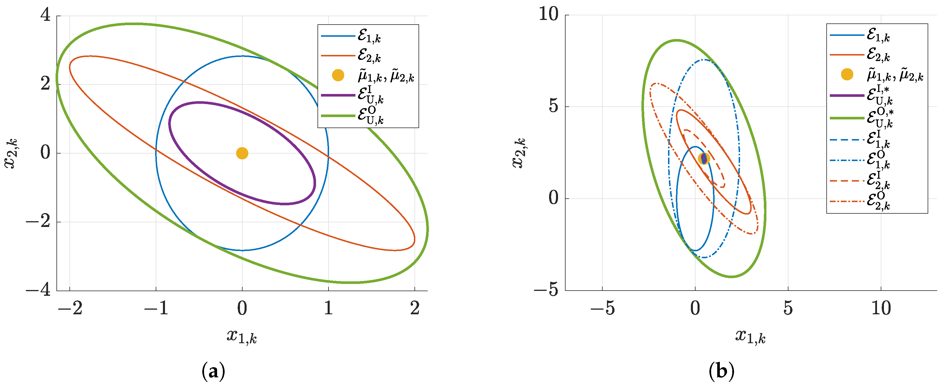
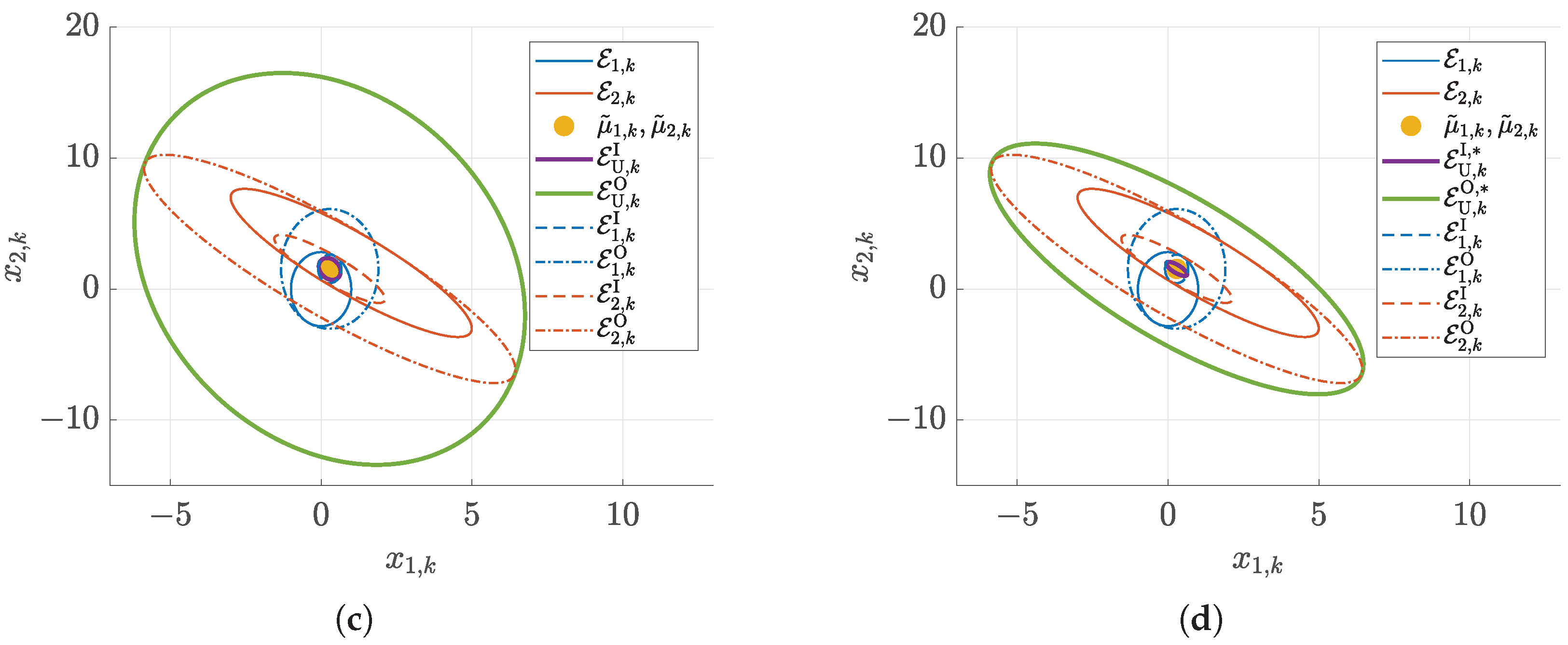
3.3. Thick Ellipsoid Union of Two Ellipsoids with Different Midpoints

3.3.1. General Solution Procedure

The thick ellipsoid union of two ellipsoids with different midpoints is a direct consequence of the procedure in Section 3.2.2. Firstly, the shape matrix Q k I of the thick ellipsoid
E U , k = E U , k μ ˜ k , Γ U , k , 1 ; η k with η k = η k * 1 and Γ U , k = Q k I 1 2
is determined as in Equation (47). The remaining degree of freedom η k * can be found according to the work of John [50]. For that purpose, specific points on the ellipsoids to be merged were extracted in [24] with subsequently inflating the inner bound by the factor η k * 1 until all points are included in its interior.
To avoid the extraction of individual points, which has to be performed with sufficient care so that the new outer bound is guaranteed to be conservative, Equation (50) with ζ j , k given in (44) is generalized to find the maximum scaling
η k * = max j { 1 , 2 } min i { 1 , , n } λ i ζ j , k 2 · Q j , k 1 · Q k I 1 2
so that all outer bounds of the thick ellipsoids in (46) are guaranteed to be contained in the union.
Remark 10.
This inflation operation generalizes naturally to an arbitrary integer number j of ellipsoids to be merged after they have been converted into representations with a common midpoint.
As an alternative parameterization (similar to the computation of the intersection of ellipsoids), both outer and inner bounds can be tuned by an alternative option. For that purpose, firstly define an approximation to the resulting shape matrix of the union according to the covariance prediction of a Kalman filter, where the state equation in the Kalman filter corresponds to computing the mean value of the data from each of the ellipsoids, with
Q ˜ k = 1 4 · Q 1 , k + Q 2 , k .
Then, the scaling factors according to (49) and (53) yield the shape matrices
Q k O , * = Q ˜ k · η k O 2 , η k O = max j { 1 , 2 } min i { 1 , , n } λ i ζ j , k 2 · Q j , k 1 · Q ˜ k 1 2
for the outer bound as well as
Q k I , * = Q ˜ k · η k I 2 , η k I = max i { 1 , , n } λ i Q k I 1 · Q ˜ k 1 2
for the inner bound.
Together, they result in the thick ellipsoid
E U , k * = E U , k * μ ˜ k , Γ U , k * , η k I ; η k O with η k = η k * 1 and Γ U , k * = Q ˜ k 1 2 .

3.3.2. Illustrating Example

Using the same examples as in (55)–(57), the procedure from Section 3.3.1 is visualized in Figure 5. Due to the fact that the outer hull in Figure 5c is more conservative than necessary (computed by means of Equation (60)), the alternative procedure from Equation (65) is preferable in the considered example. More complex options for computing optimal outer ellipsoidal enclosures typically need to employ the solution of matrix inequalities and/or minmax optimization problems in each evaluation step. Due to the resulting computational effort, such options are not further considered for the desired online application in this paper. However, the reader is referred to [19,30,56] for related work.

4. Thick Ellipsoid State Estimation Algorithm

As shown in Figure 6, the thick ellipsoid state estimation procedure consists of two stages. Prediction steps, which are based on the (uncertain) discrete-time state equation, are executed up to the point of time at which a new measurement becomes available. There, a measurement-based correction of the a-priori knowledge resulting from the previous state prediction is performed. This corrected state information then serves in a recursive manner as the input for a subsequent state prediction.

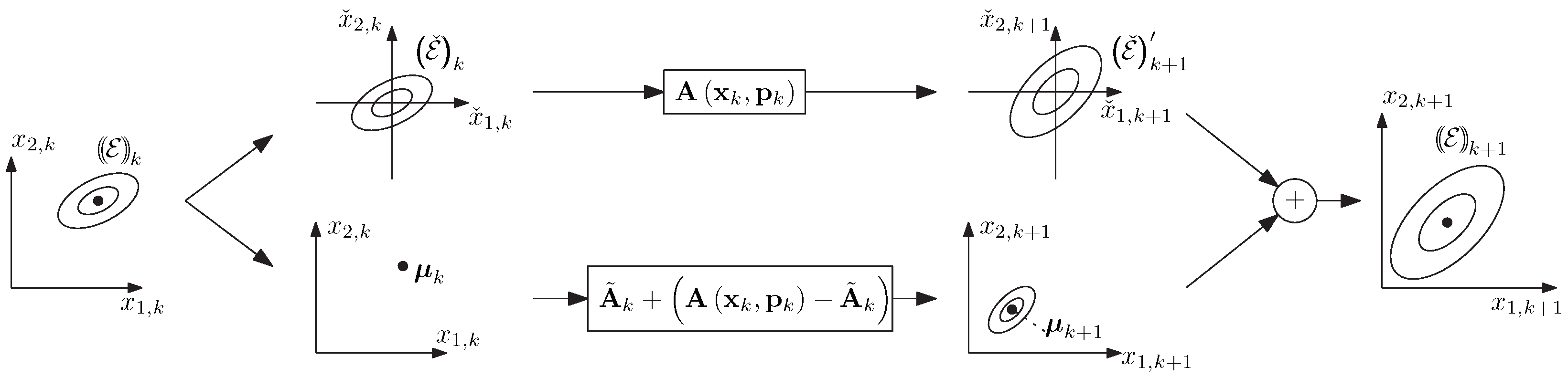
4.1. Thick Ellipsoid Prediction Step

For state estimation purposes, typically thick ellipsoids have to be considered in the prediction step according to Section 3.1 which have a non-zero midpoint. Their propagation then consists of separating the state equation as illustrated in Figure 7 into a part that depends on an ellipsoid centered at the origin and an offset term that accounts for the non-zero center according to
x k + 1 = A x k , p k · x ˇ k + A ˜ k · μ k + A x k , p k A ˜ k · μ k ,
where
x k E k μ k , Γ k , ρ ¯ k ; ρ ¯ k ,
x ˇ k E ˇ k 0 , Γ k , ρ ¯ k ; ρ ¯ k ,
A ˜ k = A μ k , mid p k , and
p k p k = p ¯ k ; p ¯ k with mid p k = 1 2 · p ¯ k + p ¯ k .
Then, the following steps are executed during the state prediction:
  • Propagate the inner bound of the thick ellipsoid (68) and extract the inner hull of the image set that is obtained by applying the mapping
    x ˇ k + 1 = A x k , p k · x ˇ k .
    Denote the corresponding shape matrix of the inner ellipsoid by Q ˇ k + 1 I . This matrix is related to the shape matrix α I , k + 1 2 · Q k + 1 in Equation (25) by
    Q ˇ k + 1 I = α I , k + 1 2 · ρ k 2 · Γ k · Γ k T .
  • Propagate the outer bound of the thick ellipsoid (68) and extract the outer hull of the image set that is obtained by applying the mapping (71). Denote the corresponding shape matrix of the outer ellipsoid by Q ˇ k + 1 O . This matrix is related to the shape matrix α O , k + 1 2 · Q k + 1 in Equation (9) by
    Q ˇ k + 1 O = α O , k + 1 2 · ρ ¯ k 2 · Γ k · Γ k T .
  • Compute interval bounds for the term
    b k = A x k , p k A ˜ k · μ k b k
    with x k , A ˜ k , and p k defined according to (67), (69), and (70) and deflate the inner ellipsoid bound as well as inflate the outer bound according to the procedure described in [20,24] with
    Q k + 1 I = 1 ρ I , k + 1 2 · Q ˇ k + 1 I , ρ I , k + 1 = sup α I , k + 1 1 · ρ ¯ k 1 · Γ k 1 · b k
    and
    1 1 Q k + 1 O = 1 + ρ O , k + 1 2 · Q ˇ k + 1 O , ρ O , k + 1 = sup α O , k + 1 1 · ρ ¯ k 1 · Γ k 1 · b k .
    Note, for ρ I 1 , the inner bound becomes the empty set.
  • Compute the updated ellipsoid midpoint as
    μ k + 1 = A ˜ k · μ k .
  • Finally, determine the predicted thick ellipsoid set
    x k + 1 E k + 1 μ k + 1 , Γ k + 1 , ρ k + 1 ; ρ ¯ k + 1 ,
    where
    ρ k + 1 = ρ k · α I , k + 1 · 1 ρ I , k + 1 , ρ ¯ k + 1 = ρ ¯ k · α O , k + 1 · 1 + ρ O , k + 1 , and Γ k + 1 = A ˜ k · Γ k .
Remark 11.
In cases where the inner ellipsoid becomes the empty set, purely the outer ellipsoid hull is further propagated to represent worst-case outer state enclosures.

4.2. Thick Ellipsoid Correction Step

The correction step of the thick ellipsoid state estimator at the point k + 1 is given by the application of Theorem 5 with the following step-by-step procedure (in this description, we prefer the version of maximized inner bounds to reduce the likelihood of empty inner enclosures; however, the task of minimizing the outer volume can be stated in full analogy):
  • Determine the inner shape matrix on the basis of Equation (47) according to
    Q k + 1 I = 2 · 2 · ξ 1 , k + 1 2 · Q k + 1 I 1 + ξ 2 , k + 1 2 · Q m , k + 1 1 1 ,
    where (based on the change of the ellipsoids’ midpoint positions according to (43)) Q k + 1 I from (75) is the inner bound of the previous prediction; Q m , k + 1 characterizes the measurement uncertainty (possibly given in terms of a degenerate ellipsoid).
  • Use Equation (48) to determine the intermediate outer bound
    Q k + 1 O = 4 · 2 · ζ 1 , k + 1 2 · Q k + 1 O 1 + ζ 2 , k + 1 2 · Q m , k + 1 1 1
    with Q k + 1 O from (76).
  • Finally, Equation (49) yields the thick Dikin ellipsoid as the result of the measurement-based correction step.

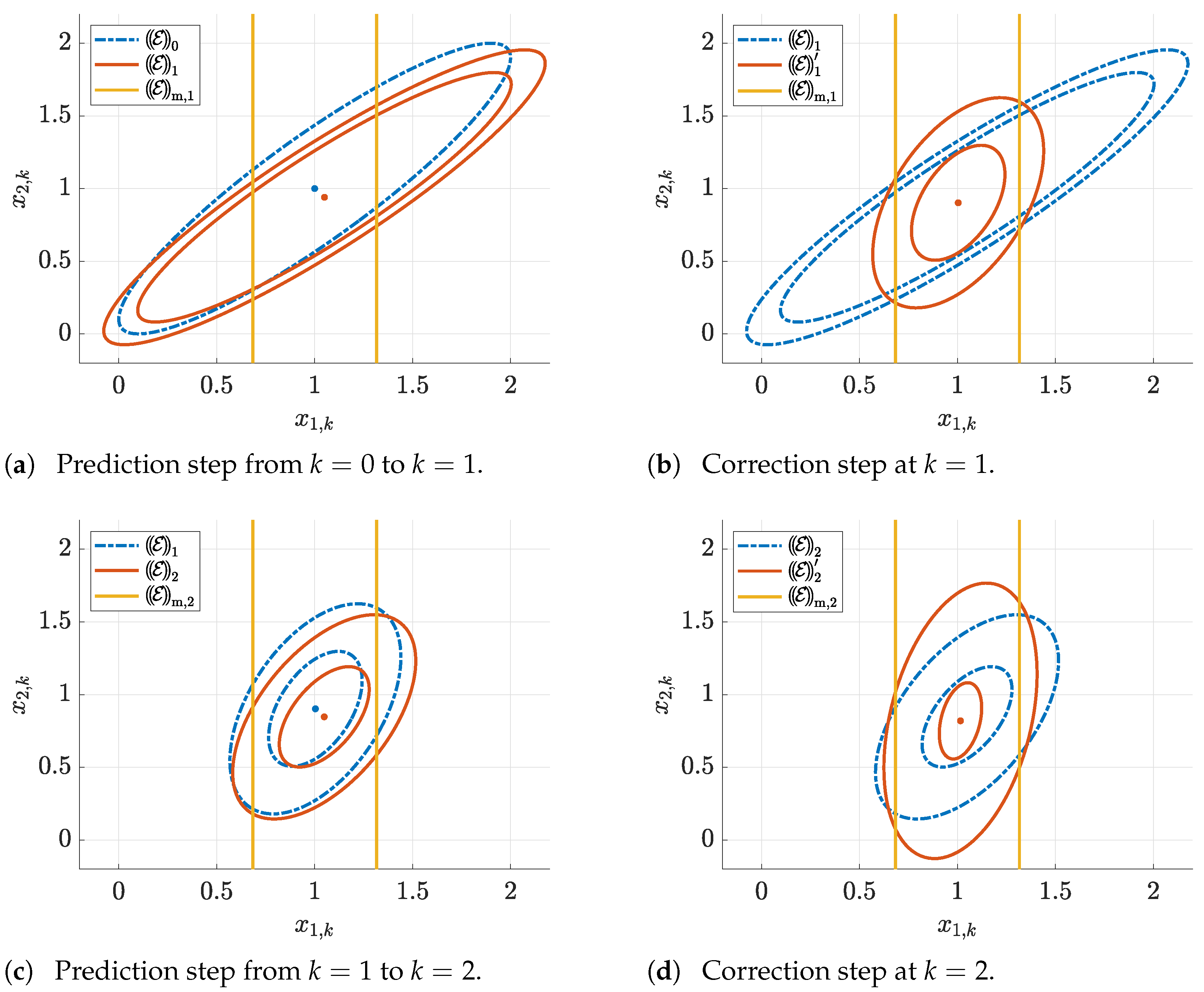
4.3. Visualization of the Thick Ellipsoid State Estimation Procedure

To visualize the individual steps of the thick ellipsoid state estimation procedure, the test example
x 1 , k + 1 x 2 , k + 1 = 1 0.05 0.01 x 1 , k 0.95 · x 1 , k x 2 , k
is investigated. At the initial point of time k = 0 , all possible system states are included in the set
E 0 = E 0 μ 0 , Γ 0 , 1 ; 1 with μ 0 = 1 1 and Γ 0 = 1 0.9 0.9 1 1 2 .
The corresponding ellipsoid is shown as the dash-dotted line in Figure 8a. Performing a single prediction step leads to a shift in the ellipsoid midpoint according to Equation (77). Moreover, the nonlinearity in the system model (82) causes the resulting distance between the inner and outer bounds of the predicted ellipsoid E 1 . Now, this ellipsoid is intersected with the measurement information that is highlighted by the vertical strip in Figure 8a,b. According to Figure 8b, the correction step leads again to a shift of the midpoint of the new thick ellipsoid E 1 according to Equations (58) and (59). The inner bound of E 1 is always fully contained in the band of possible state measurements E m , 1 , while its outer bound becomes tighter than the result of the preceding state prediction.
Now, the result E 1 serves as the input for the subsequent state prediction. For the sake of a compact notation and for compatibility with Figure 6 and Figure 7, the prime symbol is suppressed in Figure 8c, where the prediction from k = 1 to k = 2 is shown. After this prediction, the next correction step can be executed according to Figure 8d. Note, tight measurement tolerances or strongly nonlinear dependencies in the system model (re-written into the quasi-linear form) may lead to empty inner bounds after either the prediction or the correction step. Then, a slightly modified algorithm could be used. Instead of interpreting the inner bound as the state domain that is guaranteed to belong to the reachable solution set after the execution of all computations until the current instant k, it can be used to determine a measure for the precision of the sequence of prediction and correction steps at a single point of time k. For that purpose, it is necessary to initialize the inner bound of E k with the same scaling parameter as the outer bound (cf. the interval parameter with identical bounds in (83)) and to use it in analogy to the initialization of the ellipsoid in Figure 8a.

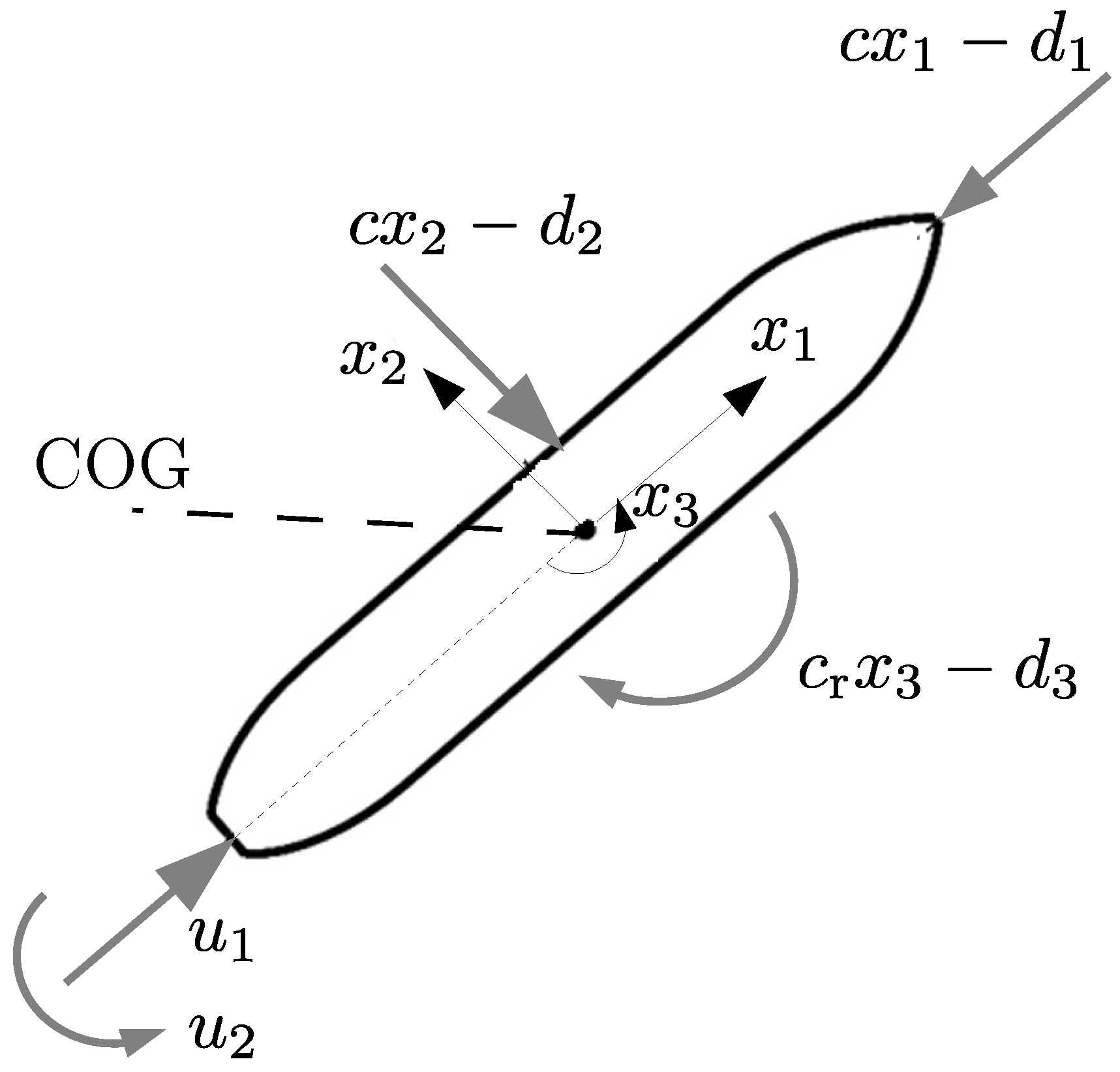
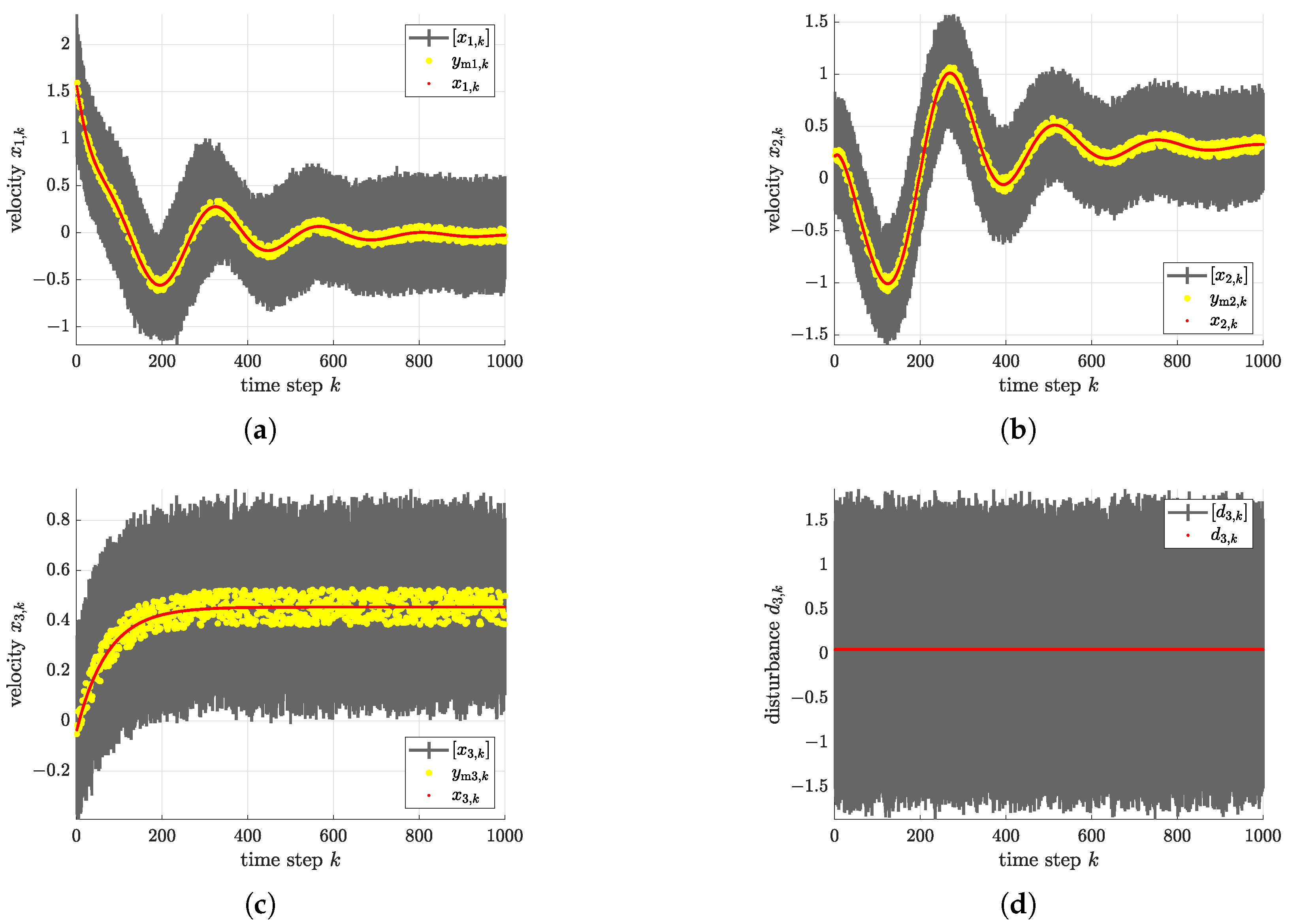
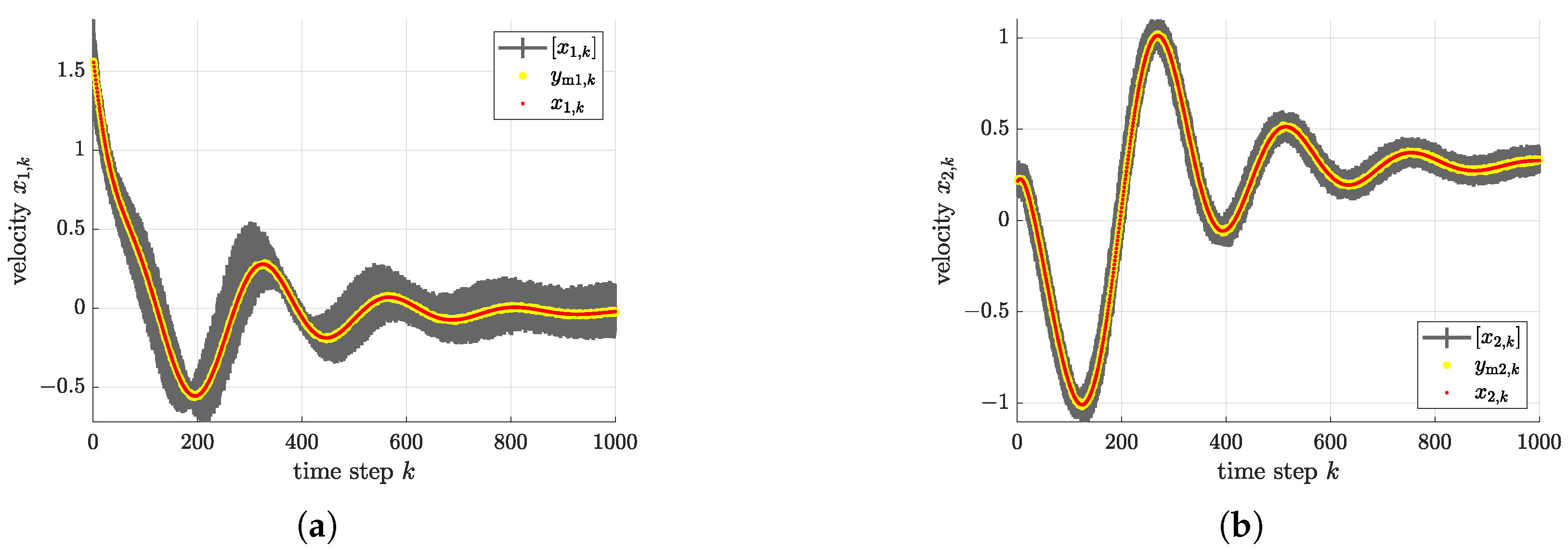
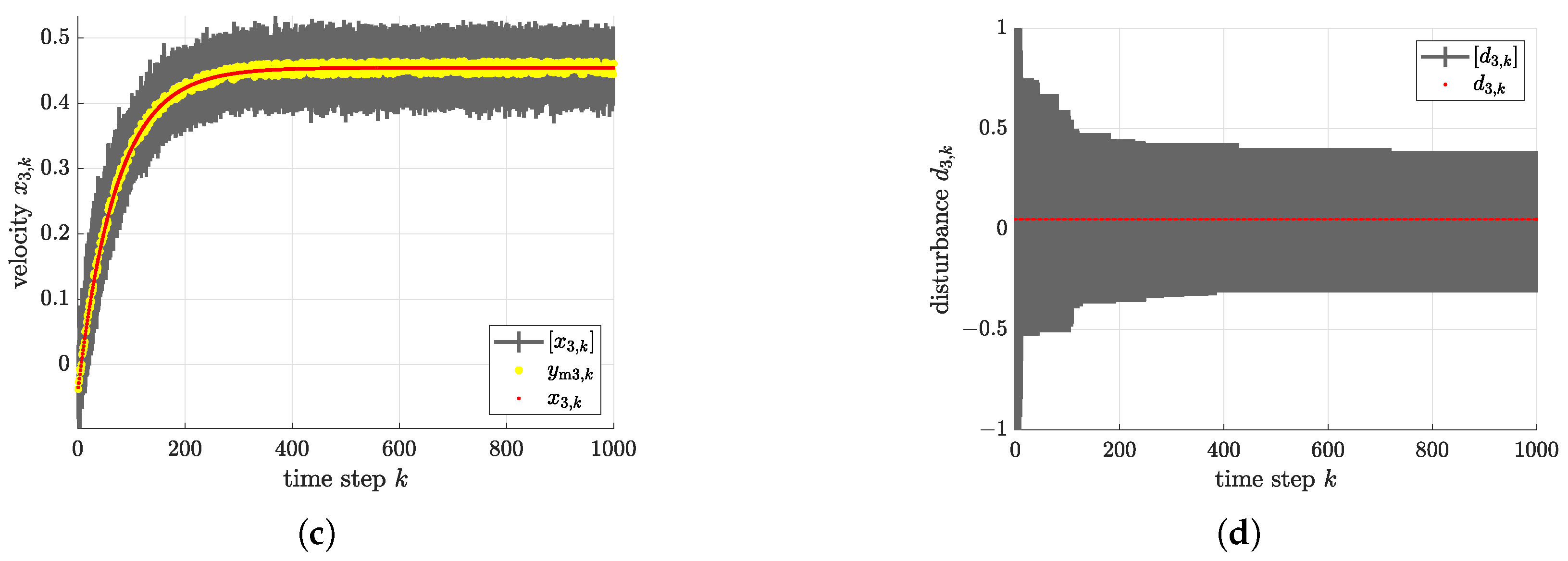
5. Application Scenario: State and Disturbance Estimation for an Underactuated Hovercraft

As a more complex benchmark application, consider the motion of an underactuated hovercraft in its body-fixed coordinate frame [57,58]. In these coordinates, it is desired to employ the ellipsoid techniques summarized in the previous sections to compute guaranteed outer state enclosures in the presence of bounded noise and disturbances. Moreover, the thick ellipsoid state estimation algorithm of Section 4 is employed to reconstruct bounds on external disturbances.

5.1. Modeling

According to Figure 9, denote the surge and sway velocities by x 1 and x 2 , respectively, and the hovercraft’s yaw rate by x 3 in a body-fixed coordinate frame. For the following derivation of the equations of motion, assume that the translational velocities are summarized in the vector V = x 1 x 2 0 T , while the angular velocity vector W with respect to the ship’s center of gravity (COG) is given by W = 0 0 x 3 T . In this formulation, the dynamics associated with the motion in heave, roll, and pitch are neglected by setting the corresponding vector entries to zero.
As also shown in [59,60], a force and torque balance in all degrees of freedom yields the equations of motion
d d t E V + W × E V = F and d d t E W + V × E V + W × E W = T ,
where
E = 1 2 · V T · m 11 0 0 0 m 22 0 0 0 m 33 · V + W T · J 11 0 0 0 J 22 0 0 0 J 33 · W
is the total kinetic energy of the ship (under the assumption of purely diagonal mass and inertia matrices [60]) with the strictly non-negative entries m i i 0 and J i i 0 , i { 1 , 2 , 3 } . For a hovercraft, it can be assumed that m 11 = m 22 = m corresponds to the mass of the ship, without additional hydrodynamic effects, while J 33 = J r is the mass moment of inertia of the vessel in the direction of x 3 .
Defining further the vectors
F = u 1 c x 1 d 1 c x 2 d 2 0 and T = 0 0 u 2 c r x 3 d 3
of non-conservative, external generalized forces and torques with the control inputs u 1 and u 2 and independent, velocity-proportional damping effects in each coordinate with the coefficient c > 0 for both translational degrees of freedom as well as c r > 0 for the rotary motion, the equations of motion (84) simplify to
x ˙ 1 x ˙ 2 x ˙ 3 d ˙ 1 d ˙ 2 d ˙ 3 = c m x 3 0 1 m 0 0 x 3 c m 0 0 1 m 0 0 0 c r J 0 0 1 J 0 0 0 0 0 0 0 0 0 0 0 0 0 0 0 0 0 0 · x 1 x 2 x 3 d 1 d 2 d 3 + 1 m 0 0 0 0 1 J 0 0 0 0 0 0 · u 1 u 2 ,
where d i , i { 1 , 2 , 3 } , represent external disturbances according to Figure 9 due to wind and currents. These disturbances are included in the state equations (87) by means of integrator disturbance models.
For the following simulation, a linear state feedback controller
u 1 u 2 = k 11 k 12 k 13 k 21 k 22 k 23 · x 1 x 2 x 3 ,
corresponding to a feedback of the actual velocity, is parameterized by means of pole assignment to decelerate the hovercraft up to standstill at the desired operating point x 1 = x 2 = x 3 = 0 .
For the use of the proposed ellipsoidal state estimation scheme, that will be applied to the closed-loop system, the state equations are discretized in time with the step size T according to
x 1 , k + 1 x 2 , k + 1 x 3 , k + 1 d 1 , k + 1 d 2 , k + 1 d 3 , k + 1 = I + T · c + k 11 m x 3 , k k 12 m k 13 m 1 m 0 0 x 3 , k c m 0 0 1 m 0 k 21 J k 22 J c r + k 23 J 0 0 1 J 0 0 0 0 0 0 0 0 0 0 0 0 0 0 0 0 0 0 · x 1 , k x 2 , k x 3 , k d 1 , k d 2 , k d 3 , k .
The (normalized) parameters used for the following simulations are: c = 0.01 , m = 5 , J = 0.8 , c r = 0.01 , k 11 = 0.5 , k 12 = 1.5 , k 13 = 0 , k 21 = 0 , k 22 = 0 , k 23 = 0.1 , and T = 0.1 .
As measured system outputs, all three velocities (surge, sway, and yaw) are assumed to be available. For the simulation, they are described by the three independent sensor models
1 δ i 2 · x i , k y m i , k 2 1 ,
where y m i , k , i { 1 , 2 , 3 } , are the data provided by the velocity sensors and δ i > 0 their corresponding maximum uncertainty. Besides filtering the velocity signals, the proposed observer is used to reconstruct the ranges of the disturbance inputs d i that are compatible with the system model and the sensor data. Due to the assumption of constant but uncertain disturbances, see Equations (87) and (89), it is permitted to intersect disturbance estimates at a specific time step k with those of previous steps and to employ those intersected results as virtual measurements in analogy to the sensor models (90).
In the system model (89), the influence of the yaw rate x 3 on the system matrix during the state prediction is accounted for by an interval parameter that corresponds to its estimated range from the preceding correction step.
Without any modification, the proposed method is capable of handling imprecisely known damping coefficients c c ; c ¯ and c r c r ; c ¯ r or uncertain masses and mass moments of inertia.

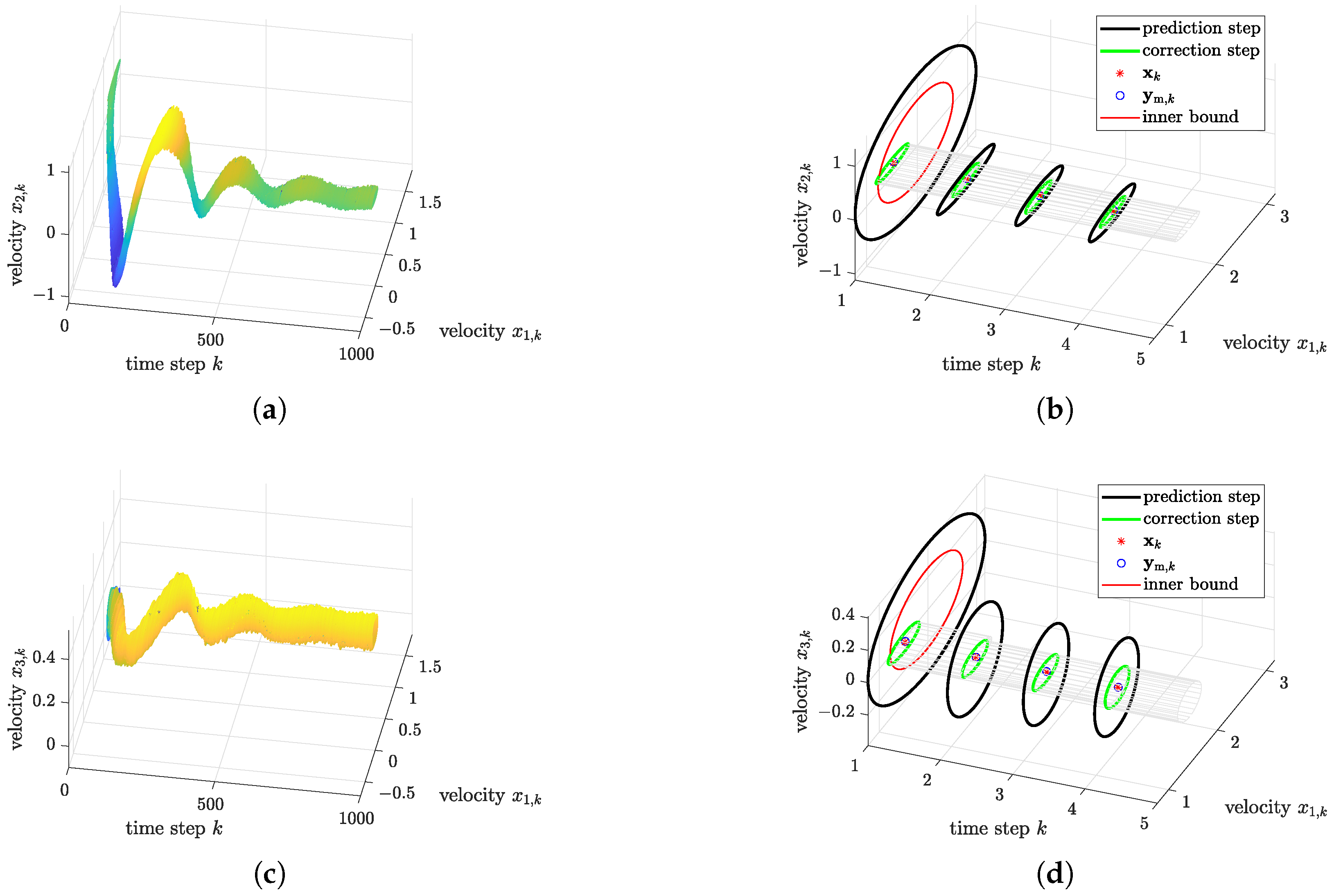
5.2. Simulation Results

To illustrate the performance of the thick ellipsoid state estimation algorithm of Section 4, two different levels of uncertainty are compared for the sensor models (90). These are
δ i 2 = 0.005 1 .
and
δ i 2 = 0.0001 .
with the help of these parameters, bounded measurement noise (in the sense of scaled uniformly distributed random numbers) has been generated for the simulations presented in this section.
Moreover, we assume true initial system states x 0 randomly chosen from the interior of an ellipsoid centered at
μ 0 * = 2 0.1 0.01 0.1 0 0 T
with the diagonal shape matrix
Q 0 * = diag 1 1 0.1 1 1 1 .
The hovercraft’s external disturbances originate from setting d 1 = 0.25 and d 3 = 0.05 .
The state estimation procedure is initialized with an ellipsoid (containing the true initial state) with the same shape matrix (94) and the shifted center μ 0 = μ 0 * 0 0 0 0.1 0 0 T .
Figure 10 and Figure 11 display the evolution of the outer state enclosures for k = 1000 steps of the estimation algorithm from Figure 6 in the left columns. In the right columns of these figures, an enlarged view is given which compares outer and inner bounds of the thick ellipsoid after the first prediction step, the propagation of the prediction results in terms of outer bounds and the respective corrected ellipsoids after accounting for the measured data. In addition, the measured and true state values are depicted.
Throughout this section, the intersection of the predicted ellipsoids with the degenerate information according to (90) is performed by the application of formula (53). The gap between the outer and inner enclosures for k = 1 indicates the non-negligible influence of nonlinearities for sufficiently uncertain values of x 3 , k . For the sake of forecasting the domains of reachable states, only the outer bounds are investigated further in Figure 12 and Figure 13. It can be seen that the smaller measurement uncertainty (92) leads to reduced uncertainty in the state reconstruction. Most noticeable, however, is the fact that the observer becomes also applicable to reconstruct bounds for the disturbance d 3 , k in this case which are tighter than their initialization and consistent with the system model as well as the uncertain state observations, cf. Figure 13d.
The disturbance estimation was performed as described at the end of the previous subsection by intersecting the current estimate for the disturbance (after the correction step) with the previously obtained best disturbance bounds.
For the case of temporally varying disturbances, this procedure has to be modified. Instead of intersecting the bounds from previous time steps, it would be necessary to account for worst-case variations of the disturbance during the prediction step by inflating the corresponding domains similarly to the influence of process noise in a Kalman filter implementation.
For the time-invariant case, future work can also aim at disturbance reconstruction by accounting for the estimates over a window of multiple time steps k and to find a common solution for the resulting set of algebraic constraints which are obtained when evaluating the state Equations (89) in which both x i , k and x i , k + 1 are replaced by the outcomes of the respective correction steps.

6. Conclusions and Outlook on Future Work

In this paper, a thick ellipsoid state estimation procedure was presented which allows for a computation of outer and (if the uncertainties are not too large) inner ellipsoidal enclosures. The advantage of the presented technique over other ellipsoidal bounding approaches such as those in [19,56] is the applicability to general (differentiable) nonlinear state equations (in this paper, in quasi-linear form) as well as its reduced complexity by using a solution technique in which complex minmax optimization procedures are replaced by simple one-parameter optimizations which only require the online computation of eigenvalues.
In future work, a combination of stochastic and set-valued uncertainty models can be investigated using the novel thick ellipsoid definitions. Other existing techniques such as those presented in [61] also make use of a Kalman filter-like structure. However, they are mainly focused on linear measurement equations. This can be circumvented by the proposed technique if the system’s output equations are reformulated in a quasi-linear form and the influence of nonlinearities is mapped onto the uncertainty that represents the measurement noise.
In addition, the simulation results in Section 5 have shown that the observer approach is capable of reconstructing bounded disturbances. This property can be exploited in future work also for an observer-based parameter identification. Finally, the thick ellipsoid-based state prediction can be employed directly for a numerical evaluation of classical Luenberger-like observers and Extended Kalman Filters. With these results, it will become possible to perform a stability analysis of these estimation schemes when applied to nonlinear dynamic systems. The procedure will be similar to the one proposed in [33], where a centered-form representation of discrete-time dynamic systems was employed for the derivation of stability contractors.

Author Contributions

The algorithm was designed jointly by A.R., A.B., and L.J. and implemented as well as validated numerically by A.R. The illustrations were made by A.R. and A.B. The paper was jointly written by A.R., A.B., and L.J. All authors have read and agreed to the published version of the manuscript.

Funding

This research received no external funding.

Conflicts of Interest

The authors declare no conflict of interest.

References

  1. Kletting, M.; Rauh, A.; Aschemann, H.; Hofer, E.P. Interval Observer Design for Nonlinear Systems with Uncertain Time-Varying Parameters. In Proceedings of the 12th IEEE International Conference on Methods and Models in Automation and Robotics MMAR, Miedzyzdroje, Poland, 28–31 August 2006; pp. 361–366. [Google Scholar]
  2. Kletting, M.; Rauh, A.; Aschemann, H.; Hofer, E.P. Interval Observer Design Based on Taylor Models for Nonlinear Uncertain Continuous-Time Systems. In Proceedings of the 12th GAMM-IMACS International Symposium on Scientific Computing, Computer Arithmetic, and Validated Numerics SCAN, Duisburg, Germany, 26–29 September 2006. [Google Scholar]
  3. Nedialkov, N.S. Interval Tools for ODEs and DAEs. In Proceedings of the 12th GAMM-IMACS International Symposium on Scientific Computing, Computer Arithmetic, and Validated Numerics SCAN, Duisburg, Germany, 26–29 September 2006. [Google Scholar]
  4. Nedialkov, N.S. Computing Rigorous Bounds on the Solution of an Initial Value Problem for an Ordinary Differential Equation. Ph.D. Thesis, Graduate Department of Computer Science, University of Toronto, Toronto, ON, Canada, 1999. [Google Scholar]
  5. Lin, Y.; Stadtherr, M.A. Validated Solutions of Initial Value Problems for Parametric ODEs. Appl. Numer. Math. 2007, 57, 1145–1162. [Google Scholar] [CrossRef] [Green Version]
  6. Berz, M.; Makino, K. Verified Integration of ODEs and Flows Using Differential Algebraic Methods on High-Order Taylor Models. Reliab. Comput. 1998, 4, 361–369. [Google Scholar] [CrossRef]
  7. Makino, K.; Berz, M. Suppression of the Wrapping Effect by Taylor Model-Based Validated Integrators; Technical Report MSU HEP 40910; Michigan State University: East Lansing, MI, USA, 2004. [Google Scholar]
  8. Goubault, E.; Mullier, O.; Putot, S.; Kieffer, M. Inner Approximated Reachability Analysis. In Proceedings of the 17th International Conference on Hybrid Systems: Computation and Control, Berlin, Germany, 15–17April 2014; pp. 163–172. [Google Scholar] [CrossRef] [Green Version]
  9. Goubault, E.; Putot, S. Robust Under-Approximations and Application to Reachability of Non-Linear Control Systems With Disturbances. IEEE Control Syst. Lett. 2020, 4, 928–933. [Google Scholar] [CrossRef]
  10. Djeumou, F.; Vinod, A.; Goubault, E.; Putot, S.; Topcu, U. On-The-Fly Control of Unknown Systems: From Side Information to Performance Guarantees through Reachability. 2020. preprint. Available online: www.researchgate.net/publication/345756893On-The-FlyControlofUnknownSystemsFromSideInformationtoPerformanceGuaranteesthroughReachability (accessed on 13 March 2021).
  11. Jaulin, L.; Kieffer, M.; Didrit, O.; Walter, É. Applied Interval Analysis; Springer: London, UK, 2001. [Google Scholar]
  12. Moore, R. Interval Arithmetic; Prentice-Hall: Englewood Cliffs, NJ, USA, 1966. [Google Scholar]
  13. Moore, R.; Kearfott, R.; Cloud, M. Introduction to Interval Analysis; SIAM: Philadelphia, PA, USA, 2009. [Google Scholar]
  14. Mayer, G. Interval Analysis and Automatic Result Verification; De Gruyter Studies in Mathematics, De Gruyter: Berlin, Germany; Boston, MA, USA, 2017. [Google Scholar]
  15. Piegat, A.; Dobryakova, L. A Decomposition Approach to Type 2 Interval Arithmetic. Int. J. Appl. Math. Comput. Sci. 2020, 30, 185–201. [Google Scholar]
  16. Desrochers, B.; Jaulin, L. Thick Set Inversion. Artif. Intell. 2017, 249, 1–18. [Google Scholar] [CrossRef] [Green Version]
  17. Măceş, D.; Stadtherr, M.A. Computing Fuzzy Trajectories for Nonlinear Dynamic Systems. Comput. Chem. Eng. 2013, 52, 10–25. [Google Scholar] [CrossRef] [Green Version]
  18. Neumaier, A. The Wrapping Effect, Ellipsoid Arithmetic, Stability and Confidence Regions. In Validation Numerics: Theory and Applications; Albrecht, R., Alefeld, G., Stetter, H.J., Eds.; Springer: Vienna, Austria, 1993; pp. 175–190. [Google Scholar]
  19. Kurzhanskii, A.B.; Vályi, I. Ellipsoidal Calculus for Estimation and Control; Birkhäuser: Boston, MA, USA, 1997. [Google Scholar]
  20. Rauh, A.; Jaulin, L. A Computationally Inexpensive Algorithm for Determining Outer and Inner Enclosures of Nonlinear Mappings of Ellipsoidal Domains. Appl. Math. Comput. Sci. AMCS 2021. under review. [Google Scholar]
  21. Wang, Y.; Puig, V.; Cembrano, G.; Zhao, Y. Zonotopic Fault Detection Observer for Discrete-Time Descriptor Systems Considering H _ Fault Sensitivity. Int. J. Syst. Sci. 2020, 1–15. [Google Scholar] [CrossRef]
  22. Zhang, W.; Wang, Z.; Raïssi, T.; Wang, Y.; Shen, Y. A State Augmentation Approach to Interval Fault Estimation for Descriptor Systems. Eur. J. Control 2020, 51, 19–29. [Google Scholar] [CrossRef]
  23. Valero, C.; Paulen, R. Set-Theoretic State Estimation for Multi-output Systems using Block and Sequential Approaches. In Proceedings of the 22nd International Conference on Process Control (PC19), Strbske Pleso, Slovakia, 11–14 June 2019; pp. 268–273. [Google Scholar]
  24. Rauh, A.; Jaulin, L. A Novel Thick Ellipsoid Approach for Verified Outer and Inner State Enclosures of Discrete-Time Dynamic Systems. In Proceedings of the 19th IFAC Symposium System Identification: Learning Models for Decision and Control, Padova, Italy, 14–16 July 2021. under review. [Google Scholar]
  25. Kalman, R.E. A New Approach to Linear Filtering and Prediction Problems. Trans. ASME J. Basic Eng. 1960, 82, 35–45. [Google Scholar] [CrossRef] [Green Version]
  26. Daum, F. Nonlinear Filters: Beyond the Kalman Filter. IEEE Aerosp. Electron. Syst. Mag. 2005, 20, 57–69. [Google Scholar] [CrossRef]
  27. Julier, S.; Uhlmann, J.; Durrant-Whyte, H. A New Approach for the Nonlinear Transformation of Means and Covariances in Filters and Estimators. IEEE Trans. Autom. Control 2000, 45, 477–482. [Google Scholar] [CrossRef] [Green Version]
  28. Rauh, A.; Briechle, K.; Hanebeck, U.D. Nonlinear Measurement Update and Prediction: Prior Density Splitting Mixture Estimator. In Proceedings of the 2009 IEEE Control Applications, (CCA) & Intelligent Control, (ISIC), St. Petersburg, Russia,, 8–10 July 2009. [Google Scholar]
  29. Hanebeck, U.D.; Briechle, K.; Rauh, A. Progressive Bayes: A New Framework for Nonlinear State Estimation. In Multisensor, Multisource Information Fusion: Architectures, Algorithms, and Applications 2003; Dasarathy, B.V., Ed.; International Society for Optics and Photonics, SPIE: Orlando, FL, USA, 2003; Volume 5099, pp. 256–267. [Google Scholar]
  30. Jambawalikar, S.; Kumar, P. A Note on Approximate Minimum Volume Enclosing Ellipsoid of Ellipsoids. In Proceedings of the 2008 International Conference on Computational Sciences and Its Applications, Perugia, Italy, 30 June–3 July 2008; pp. 478–487. [Google Scholar] [CrossRef] [Green Version]
  31. Halder, A. On the Parameterized Computation of Minimum Volume Outer Ellipsoid of Minkowski Sum of Ellipsoids. In Proceedings of the IEEE Conference on Decision and Control (CDC), Miami, FL, USA, 17–19 December 2018; pp. 4040–4045. [Google Scholar] [CrossRef] [Green Version]
  32. Yildirim, E.A. On the Minimum Volume Covering Ellipsoid of Ellipsoids. SIAM J. Optim. 2006, 17, 621–641. [Google Scholar] [CrossRef] [Green Version]
  33. Bourgois, A.; Jaulin, L. Interval Centred Form for Proving Stability of Non-Linear Discrete-Time Ssystems. In Proceedings of the 6th International Workshop on Symbolic-Numeric methods for Reasoning about CPS and IoT, Online, 31 August 2020; 2021; pp. 1–17. [Google Scholar] [CrossRef]
  34. Chapoutot, A. Interval Slopes as a Numerical Abstract Domain for Floating-Point Variables. In Static Analysis; Lecture Notes in Computer Science; Springer: Berlin/Heidelberg, Germany, 2010; pp. 184–200. [Google Scholar]
  35. Cornelius, H.; Lohner, R. Computing the Range of Values of Real Functions with Accuracy Higher Than Second Order. Computing 1984, 33, 331–347. [Google Scholar] [CrossRef]
  36. Scherer, C.; Weiland, S. Linear Matrix Inequalities in Control. In Control System Advanced Methods, 2nd ed.; Levine, W.S., Ed.; The Electrical Engineering Handbook Series; CRC Press: Boca Raton, FL, USA, 2011; pp. 24-1–24-30. [Google Scholar]
  37. Boyd, S.; El Ghaoui, L.; Feron, E.; Balakrishnan, V. Linear Matrix Inequalities in System and Control Theory; SIAM: Philadelphia, PA, USA, 1994. [Google Scholar]
  38. Sturm, J. Using SeDuMi 1.02, A MATLAB Toolbox for Optimization over Symmetric Cones. Optim. Methods Softw. 1999, 11–12, 625–653. [Google Scholar] [CrossRef]
  39. Löfberg, J. YALMIP: A Toolbox for Modeling and Optimization in MATLAB. In Proceedings of the IEEE International Symposium on Computer Aided Control Systems Design, Taipei, Taiwan, 2–4 September 2004; pp. 284–289. [Google Scholar]
  40. Cichy, B.; Gałkowski, K.; Dąbkowski, P.; Aschemann, H.; Rauh, A. A New Procedure for the Design of Iterative Learning Controllers Using a 2D Systems Formulation of Processes with Uncertain Spatio-Temporal Dynamics. Control Cybern. 2013, 42, 9–26. [Google Scholar]
  41. Barmish, B.R. New Tools for Robustness of Linear Systems; Macmillan: New York, NY, USA, 1994. [Google Scholar]
  42. Rump, S. IntLab—INTerval LABoratory; Developments in Reliable Computing; Csendes, T., Ed.; Kluwer Academic Publishers: New York, NY, USA, 1999; pp. 77–104. [Google Scholar]
  43. Durieu, C.; Polyak, B.T.; Walter, E. Trace Versus Determinant in Ellipsoidal Outer-Bounding, with Application to State Estimation. IFAC Proc. Vol. 1996, 29, 3975–3980. [Google Scholar] [CrossRef]
  44. Dabbene, F.; Henrion, D. Set Approximation via Minimum-Volume Polynomial Sublevel Sets. In Proceedings of the 2013 European Control Conference (ECC), Zurich, Switzerland, 17–19 July 2013; pp. 1114–1119. [Google Scholar]
  45. Tarbouriech, S.; Garcia, G.; Gomes da Silva, J.; Queinnec, I. Stability and Stabilization of Linear Systems with Saturating Actuators; Springer: London, UK, 2011. [Google Scholar]
  46. Rohn, J. Bounds on Eigenvalues of Interval Matrices. Zamm J. Appl. Math. Mech./Z für angew. Math. und Mech. 1998, 78, 1049–1050. [Google Scholar] [CrossRef] [Green Version]
  47. Paradowski, T.; Lerch, S.; Damaszek, M.; Dehnert, R.; Tibken, B. Observability of Uncertain Nonlinear Systems Using Interval Analysis. Algorithms 2020, 13, 66. [Google Scholar] [CrossRef] [Green Version]
  48. Weinmann, A. Uncertain Models and Robust Control; Springer: Wien, Austria, 1991. [Google Scholar]
  49. Henrion, D.; Tarbouriech, S.; Arzelier, D. LMI Approximations for the Radius of the Intersection of Ellipsoids: Survey. J. Optim. Theory Appl. 2001, 108, 1–28. [Google Scholar] [CrossRef]
  50. John, F. Extremum Problems with Inequalities as Subsidiary Conditions. In Studies and Essays Presented to R. Courant on His 60th Birthday; Interscience Publishers, Inc.: New York, NY, USA, 1948; pp. 187–204. [Google Scholar]
  51. Roos, C.; Terlaky, T.; Nemirovski, A.; Roos, K. On Maximization of Quadratic form over Intersection of Ellipsoids with Common Center. Math. Program. 1999, 86. [Google Scholar] [CrossRef] [Green Version]
  52. Gilitschenski, I.; Hanebeck, U.D. A Robust Computational Test for Overlap of Two Arbitrary-dimensional Ellipsoids in Fault-Detection of Kalman Filters. In Proceedings of the15th International Conference on Information Fusion, Singapore, 9–12 July 2012. [Google Scholar]
  53. Gilitschenski, I.; Hanebeck, U.D. A Direct Method for Checking Overlap of Two Hyperellipsoids. In Proceedings of the IEEE ISIF Workshop on Sensor Data Fusion: Trends, Solutions, Applications, Bonn, Germany, 8–10 October 2014. [Google Scholar]
  54. Becis-Aubry, Y. Ellipsoidal Constrained State Estimation in Presence of Bounded Disturbances. 2020. Available online: arxiv.org/pdf/2012.03267v1.pdf (accessed on 13 March 2021).
  55. Stengel, R. Optimal Control and Estimation; Dover Publications, Inc.: New York, NY, USA, 1994. [Google Scholar]
  56. Kurzhanskiy, A.; Varaiya, P. Ellipsoidal Toolbox (ET). In Proceedings of the 45th IEEE Conference on Decision and Control, San Diego, CA, USA, 13–15 December 2006; pp. 1498–1503. [Google Scholar]
  57. Rauh, A.; Grigoryev, V.; Aschemann, H.; Paschen, M. Incremental Gain Scheduling and Sensitivity-Based Control for Underactuated Ships. In Proceedings of the IFAC Conference on Control Applications in Marine Systems, CAMS, Rostock-Warnemunde, Germany, 15–17 September 2010. [Google Scholar]
  58. Rauh, A. Sensitivity Methods for Analysis and Design of Dynamic Systems with Applications in Control Engineering; Shaker: Düren, Germany, 2017. [Google Scholar]
  59. Fossen, T. Guidance and Control of Ocean Vehicles; John Wiley & Sons: Chichester, UK, 1994. [Google Scholar]
  60. Reyhanoglu, M. Exponential Stabilization of an Underactuated Autonomous Surface Vessel. Automatica 1997, 33, 2249–2254. [Google Scholar] [CrossRef] [Green Version]
  61. Pfaff, F.; Noack, B.; Hanebeck, U.D. Data Validation in the Presence of Stochastic and Set-membership Uncertainties. In Proceedings of the 16th International Conference on Information Fusion, Istanbul, Turkey, 9–12 July 2013. [Google Scholar]
Figure 1. Definition of a thick ellipsoid E k enclosing the domain A k and its mapping via the system model (2).
Algorithms 14 00088 g001
Figure 2. Computation of the thick ellipsoid enclosure E k + 1 for the example (35). The exact inner solution sets are visualized in light gray color, while the dark gray domains consist of the union of ellipsoid bounds that result from a numerical mapping of a 20 × 20 grid for the interval parameters p 1 and p 2 .
Algorithms 14 00088 g002
Figure 3. Intersection of ellipsoids E 1 , k and E 2 , k with identical and different midpoints. Inner bound of the resulting thick ellipsoid: E D , k I ; outer bound: E D , k O (∗ symbols denote the solution enclosure according to Equation (53)). (a) Case according to Section 3.2.1 with the shape matrices (55). (b) Case according to Section 3.2.2 with the initial ellipsoid parameterization (55), (56), enclosure definition (53). (c) Case according to Section 3.2.2 with the initial ellipsoid parameterization (56), (57), enclosure definition (49). (d) Case according to Section 3.2.2 with the initial ellipsoid parameterization (56), (57), enclosure definition (53).
Algorithms 14 00088 g003
Figure 4. Intersection of an ellipsoid E 1 , k with the degenerate ellipsoid E 2 , k (vertical strip) with identical and different midpoints. Inner bound of the resulting thick ellipsoid: E D , k I ; outer bound: E D , k O (∗ symbols denote the solution enclosure according to Equation (53)). (a) Case according to Section 3.2.1 with Q 2 , k according to (55). (b) Case according to Section 3.2.2 with the initial ellipsoid parameterization (56), (57), enclosure definition (49). (c) Case according to Section 3.2.2 with the initial ellipsoid parameterization (56), (57), enclosure definition (53).
Algorithms 14 00088 g004
Figure 5. Union of ellipsoids E 1 , k and E 2 , k with identical and different midpoints. Inner bound of the resulting thick ellipsoid: E U , k I ; outer bound: E U , k O (∗ symbols denote the solution enclosure according to Equation (65)). (a) Union of ellipsoids with identical midpoints, cf. (55). (b) Union of ellipsoids with the initial ellipsoid parameterization (55), (56), enclosure definition (65). (c) Union of ellipsoids with the initial ellipsoid parameterization (56), (57), enclosure definition (60). (d) Union of ellipsoids with the initial ellipsoid parameterization (56), (57), enclosure definition (65).
Algorithms 14 00088 g005aAlgorithms 14 00088 g005b
Figure 6. Thick ellipsoid state estimation algorithm consisting of prediction and correction stages.
Algorithms 14 00088 g006
Figure 7. Separation of the state equations according to (66)–(70) into the mapping of an origin-centered ellipsoid and the verified treatment of non-zero offset terms.
Algorithms 14 00088 g007
Figure 8. Visualization of the thick ellipsoid state estimation procedure for the example system in (82).
Algorithms 14 00088 g008
Figure 9. Definition of the velocity components in a body-fixed coordinate systems, velocity-proportional damping as well as disturbance forces and torques.
Algorithms 14 00088 g009
Figure 10. State estimation for the case of large uncertainties (91). (a) Outer ellipsoidal enclosures for the velocities x 1 , k and x 2 , k . (b) Enlarged view of the ellipsoidal enclosures of x 1 , k and x 2 , k . (c) Outer ellipsoidal enclosures for the velocities x 1 , k and x 3 , k . (d) Enlarged view of the ellipsoidal enclosures of x 1 , k and x 3 , k .
Algorithms 14 00088 g010
Figure 11. State estimation for the case of small uncertainties (92). (a) Outer ellipsoidal enclosures for the velocities x 1 , k and x 2 , k . (b) Enlarged view of the ellipsoidal enclosures of x 1 , k and x 2 , k . (c) Outer ellipsoidal enclosures for the velocities x 1 , k and x 3 , k . (d) Enlarged view of the ellipsoidal enclosures of x 1 , k and x 3 , k .
Algorithms 14 00088 g011
Figure 12. Comparison of the estimation results with noisy measurements and true system states for the case of large uncertainties (91). (a) Estimated bounds x 1 , k vs. measured and true velocities y m 1 , k and x 1 , k . (b) Estimated bounds x 2 , k vs. measured and true velocities y m 2 , k and x 2 , k . (c) Estimated bounds x 3 , k vs. measured and true velocities y m 3 , k and x 3 , k . (d) Estimated bounds d 3 , k vs. true disurbance d 3 , k = 0.05 .
Algorithms 14 00088 g012
Figure 13. Comparison of the estimation results with noisy measurements and true system states for the case of small uncertainties (92). (a) Estimated bounds x 1 , k vs. measured and true velocities y m 1 , k and x 1 , k . (b) Estimated bounds x 2 , k vs. measured and true velocities y m 2 , k and x 2 , k . (c) Estimated bounds x 3 , k vs. measured and true velocities y m 3 , k and x 3 , k . (d) Estimated bounds d 3 , k vs. true disurbance d 3 , k = 0.05 .
Algorithms 14 00088 g013aAlgorithms 14 00088 g013b
Publisher’s Note: MDPI stays neutral with regard to jurisdictional claims in published maps and institutional affiliations.

