
3D Mesh Model Classification with a Capsule Network

1
Faculty of Electrical Engineering and Computer Science, Ningbo University, Ningbo 315211, China
2
Mobile Network Application Technology Key Laboratory of Zhejiang Province, Ningbo 315211, China
*
Author to whom correspondence should be addressed.
Algorithms 2021, 14(3), 99; https://0-doi-org.brum.beds.ac.uk/10.3390/a14030099
Submission received: 1 March 2021
/
Revised: 17 March 2021
/
Accepted: 20 March 2021
/
Published: 22 March 2021
Abstract
:With the widespread success of deep learning in the two-dimensional field, how to apply deep learning methods from two-dimensional to three-dimensional field has become a current research hotspot. Among them, the polygon mesh structure in the three-dimensional representation as a complex data structure provides an effective shape approximate representation for the three-dimensional object. Although the traditional method can extract the characteristics of the three-dimensional object through the graphical method, it cannot be applied to more complex objects. However, due to the complexity and irregularity of the mesh data, it is difficult to directly apply convolutional neural networks to 3D mesh data processing. Considering this problem, we propose a deep learning method based on a capsule network to effectively classify mesh data. We first design a polynomial convolution template. Through a sliding operation similar to a two-dimensional image convolution window, we directly sample on the grid surface, and use the window sampling surface as the minimum unit of calculation. Because a high-order polynomial can effectively represent a surface, we fit the approximate shape of the surface through the polynomial, use the polynomial parameter as the shape feature of the surface, and add the center point coordinates and normal vector of the surface as the pose feature of the surface. The feature is used as the feature vector of the surface. At the same time, to solve the problem of the introduction of a large number of pooling layers in traditional convolutional neural networks, the capsule network is introduced. For the problem of nonuniform size of the input grid model, the capsule network attitude parameter learning method is improved by sharing the weight of the attitude matrix. The amount of model parameters is reduced, and the training efficiency of the 3D mesh model is further improved. The experiment is compared with the traditional method and the latest two methods on the SHREC15 data set. Compared with the MeshNet and MeshCNN, the average recognition accuracy in the original test set is improved by 3.4% and 2.1%, and the average after fusion of features the accuracy reaches 93.8%. At the same time, under the premise of short training time, this method can also achieve considerable recognition results through experimental verification. The three-dimensional mesh classification method proposed in this paper combines the advantages of graphics and deep learning methods, and effectively improves the classification effect of 3D mesh model.
1. Introduction
As one of the most representative neural networks in the field of deep learning technology, convolutional neural networks have made many breakthroughs in popular tasks such as image classification and semantic segmentation. Three-dimensional image data contain more information than 2D image data; they are richer and have better illumination invariance and posture invariance, so how to apply deep learning to the representation of three-dimensional models has become a research hotspot in the field of digital geometry [1].
1.1. Problem Description and Existing Work
At present, the data formats of three-dimensional model recognition methods mainly include the voxel form, the point cloud form and the three-dimensional grid representation.
For voxel representation, 3DShapeNets [2] proposed by Wu et al. and VoxNet [3] proposed by Maturana and Scherer et al. both directly learn on voxels and divide the space into regular cubes. However, due to the sparseness of voxel data, it introduces additional computational cost, which limits the method from being applied to complex datasets. FPNN [4] proposed by Li et al., Vote3D [5] proposed by Wang and Posner et al. and the Octtree-based convolutional neural network (OCNN) [6] proposed by Wang et al. solve the problem of the sparseness of voxel data. Compared with two-dimensional convolution, the use of three-dimensional convolution adds a spatial dimension, the memory requirements become too large, and the entire method is limited by the size of the input data.
For point cloud representation, due to the disorder of the point cloud data, the usual network framework is not suitable for a direct application of the point cloud data. Qi et al. proposed PointNet [7] in 2017, which solved the problem through a symmetric function, but it ignored the point cloud local information. Qi and others later proposed PointNet++ [8], an improved version of PointNet, which added an aggregation operation with neighbors to solve this problem. Because the point cloud data structure is too simple, for two compact nonconnected surfaces, the local surface cannot be distinguished simply by the Euclidean distance, so it cannot represent a complex model well.
The mesh representation is a collection of points, faces, and edges, which are topologically combined through triangular patches, which can accurately express the neighborhood information of the points and has the natural advantage of expressing the complex surface of the object. However, the grid data are more complicated and the ordinary convolution operation cannot be directly applied to the mesh model, and there are currently few deep learning methods based on the mesh model. Hanocka, Hertz et al. proposed MeshCNN [9] in 2019 to define the convolution with an edge as the center of two triangles. The ratio of the dihedral angle, the inner angle, and the height of the triangle to the bottom edge is used as a five-dimensional feature vector, which is pooled by edge folding to apply the convolution network to the grid structure. Feng et al. proposed Mesh-Net (2019) [10], taking triangular patches as the smallest unit; extracting its center point coordinates, normal vectors, neighborhood polygon index and other features; designing a convolutional neural network for classification; and achieving a recognition rate of 91.9% for the ModelNet40 data set. Yang et al. proposed a mesh grid-based convolution framework PFCNN [11], which constructed a new translation structure by using multiple directions of parallel frame field to encode plane connections on the surface to ensure the translation of convolution. Degeneration is more accurate than surface-based CNN in terms of fine-scale feature learning. In 2020, Wang et al. proposed the first method of grid pose conversion through style conversion [12], through spatial adaptive instance normalization (SPAdaIN) To simulate image pixels and mesh vertices. Learn the pose characteristics of each vertex in the source mesh and use the affine transformation learned from the target mesh vertices to transform it, thereby effectively transferring the pose of the source mesh to the target mesh Geshang.Qiao et al. proposed LaplacianNet [13] in 2020, which performs multi-scale pooling on the basis of Laplacian spectral clustering, and uses grid pooling blocks to utilize global information after pooling, and introduces a The correlation network is used to calculate the correlation matrix, which aggregates global features by multiplying with the matrix of clustering features, and achieves good results on the ShapeNet and COSEG data sets. Litany et al. proposed a learning-based method to complete the three-dimensional graph generation and completion [14]. The reference shape and latent space parameters are constructed by training a graph convolutional variational autoencoder. When inferring, only the decoder and part of the missing shape are used as input, and correspond to the reference shape, reconstruction human body and face mesh.
Most of the above methods use CNN to complete classification and segmentation or other tasks. Although the CNN is successful on most tasks, it also has some limitations, mainly due to its data routing process. In the process of data forward propagation, CNN uses operations such as maximum pooling or average pooling to obtain image transformation invariance, more compact representation, and better noise and clustering robustness [15]. MeshNet, for example, uses maximum pooling in the aggregation module to provide a form of translation invariance, resulting in the loss of valuable spatial information between neural layers. These pooling operations discard high-level features. The relative positional relationship between the other parameter information of the layer and the encoded features. For example, for the “Picasso problem” in image recognition (an image that has all the correct parts but does not have the correct spatial relationship), CNN will still recognize the face, but will not care. The composition of the structural relationship between the parts that make up the face.
1.2. Motivation and Contribution
In order to overcome the above problems of CNN, Hinton et al. proposed a new algorithm called capsule network [16]. Routing replaces the maximum pooling down sampling in CNN, saves feature information of different dimensions, and reuses the output of some of these capsules to form a more stable high-order capsule representation [17], which better preserves the space of features information. At present, experiments have verified the advantages of capsule network compared with CNN in two-dimensional image classification [18]. In terms of application, Iesmantas et al. applied the capsule network based on binary classification to the detection of breast cancer [19]. Jaiswal et al. designed a capsule-based GAN [20]. Yang et al. applied the capsule network to the text domain [21]. Nguyen et al. applied the capsule network to digital media forensics [22].
Recently, the capsule network has gradually been applied to the point cloud field to promote the development of computer graphics. Based on the combination of Euclidean, eigenvalues and geometrical space features, a dynamic capsule graph convolution network DCG-Net [23] was proposed. As the first method of using the capsule network architecture for point cloud edge detection, EDC-Net [24] is based on the extracted feature graph, by applying the attention module to the main capsule, and redesigning the loss function to obtain better results. Aiming at CNNs cannot sufficiently address the spatial relationship between features and require large amounts of data for training, the 3D point capsule networks [25] by Zhao and the method by Ahmad [26] were proposed. They extended the capsule network to the three-dimensional field by 3D convolution and verified its effectiveness through experiments.
These studies proved the effectiveness of the capsule network in many fields. However, due to the complex 3D mesh model data, no capsule network has been applied to 3D mesh processing, which prompted us to continue to develop a method for effective analysis of 3D mesh data.
This paper proposes a three-dimensional mesh classification method based on capsule network, 3D Mesh Capsule Networks (MeshCaps), to expand the application field of capsule network. As the first method to apply capsule network to three-dimensional mesh structure, MeshCaps is similar to traditional multilayer neural networks can run directly on irregular grids, and can extract high-level features through a multilayer network structure.
In MeshCaps, the mesh surface is convolved through the designed convolution template. Since the polynomial can effectively express a surface and the representation is more concise, the convolution kernel is designed as a high-order equation, and the polynomial fitting is used in the window. In the surface method, the high-order equation parameters are used as the local features of the window surface, which enables this method to deal with the complexity and irregular shape of the grid according to the surface unit.
In addition, considering the inconsistency of the input size of the three-dimensional grid model, a capsule network that shares the weights of the pose matrix is introduced, and the concept of the capsule network is extended to the three-dimensional grid model. Based on these ideas, this paper designs a network structure in which is included a polynomial template convolution kernel used to learn feature descriptors of the patch unit and a capsule network used to aggregate and classify adjacent hidden layer features. Compared with the latest method MeshCNN based on edge folding for convolution pooling, it is expected that the improved capsule network will achieve better classification results under more expressive polynomial features.
1.3. Structure of the Paper
The rest of this paper is organized as follows. In Section 2, we give a technical description of the two-dimensional capsule network problem. The proposed 3D Mesh model classification algorithm is described in Section 3. In Section 4, we introduce and discuss the experimental results. Finally, Section 5 summarizes the work and provides guidance for future work.
2. 2D Capsule Networks
As mentioned earlier, the goal of this article is to study and design a network architecture for a three-dimensional grid, which is based on a capsule network. First, let’s introduce the characteristics of the capsule network.
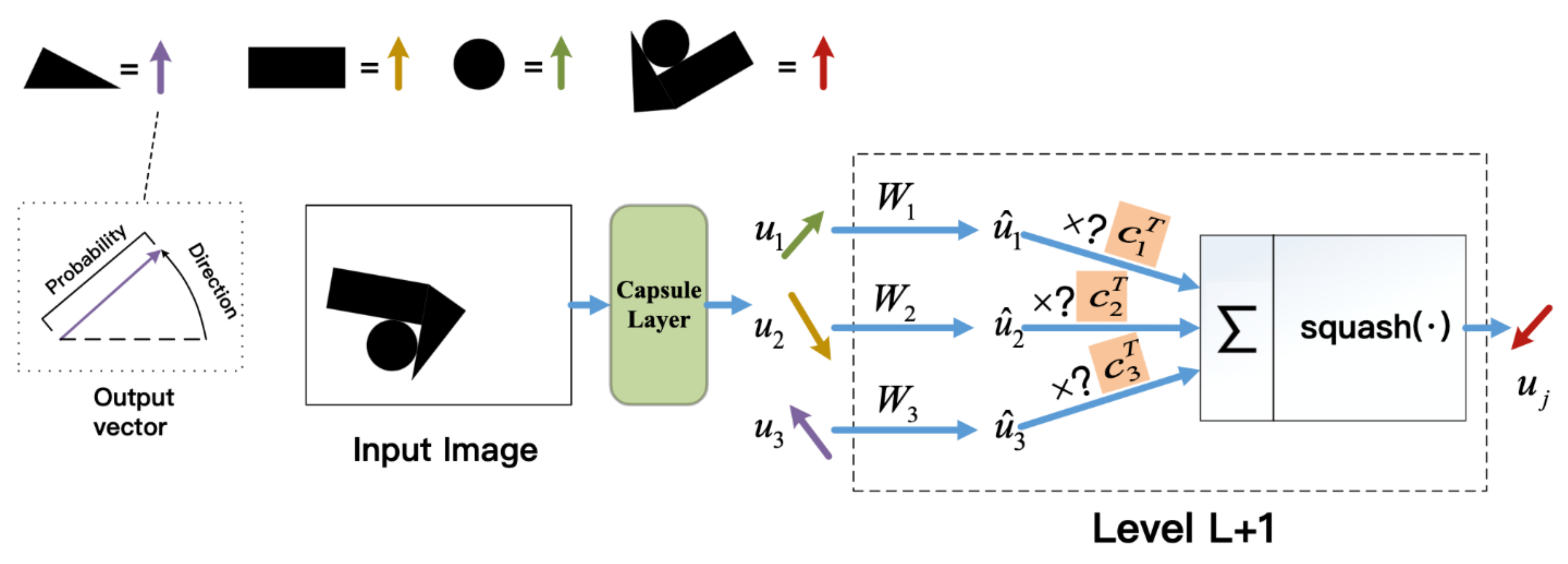
The capsule network is composed of multiple capsule layers, where the capsule is an independent logical unit and represents a whole or part of the whole through a vector. Compared with the traditional CNN input and output in the form of scalar, the input and output of the capsule network are in the form of vector. Each dimension of the vector can be expressed as a feature pattern (such as deformation, posture, reflectivity, texture, etc.), and the norm of the feature vector is used to express the confidence of the entity’s existence. It can not only perform feature detection based on statistical information, but also learn to understand the positional relationship between the part and the whole and understand the representation mode of the dimension in the feature vector.
The capsule network performs a large number of operations inside the capsule and uses the protocol routing algorithm to output a high-dimensional vector upwards to ensure that the capsule output is sent to the corresponding high-level capsule in the next layer. The operation method in a single capsule is shown in Figure 1. When the layer capsule passes the feature vector learned and predicted by itself to the higher-level capsule, if the prediction is consistent, the corresponding c value increases, and the higher-level capsule is activated. With the continuous iteration of the dynamic routing mechanism, it can train various capsules into units that learn different dimensions to identify the correct category of the image.
Unlike the maximum pooling of CNN, the capsule network does not discard the information about the precise position of the entity in the area. Before the capsule is passed to the next layer, a transformation of the pose matrix W must be performed, and the parameters of W are learned through gradient descent. In order to make the network have the ability to identify features from multiple angles. For low-level capsules, the position information is “encoded”. As the hierarchical structure is improved, more and more position information is “compressed and encoded” into the real-valued components of the capsule output vector.
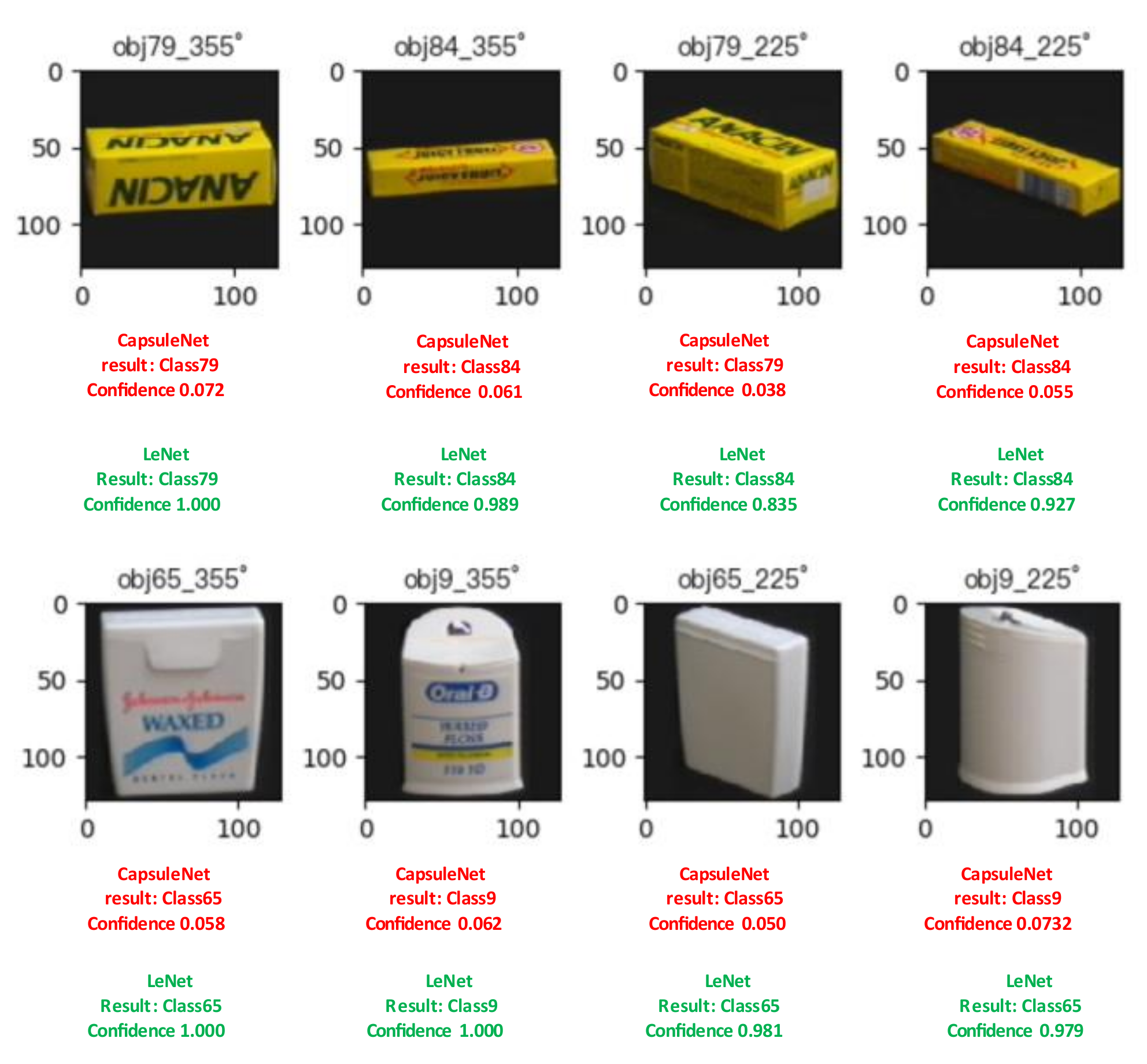
Under the Coil-100 rotating data set, this paper did a preliminary experiment to compare the recognition ability of LeNet [27] and the capsule network for objects at different angles. Among them, LeNet consists of two 5 × 5 convolution kernels and three fully connected layers. The capsule network follows the network design in the original paper. Select 0, 30, 60, 90, 120, 160, and 180 degree images as the training data, set the initial learning rate to 0.001, and batch size to 64 to train 50 epochs, and test the classification of different objects at 225–355 angles.
As shown in Figure 2, LeNet has misjudgments for the images in the third column of the first row and the fourth column of the second row. For objects with different angles, the capsule network can still accurately identify objects with low confidence. obj79_355° indicates the 79th type of image rotated by 355 degrees, and the red and green text indicate the results of the capsule network and LeNet classification respectively.
Compared with the two-dimensional image, the data of the three-dimensional model is more complicated. This paper designs a capsule network framework for the three-dimensional mesh model.
3. 3D Mesh Capsule Networks
This section introduces the design of MeshCaps in detail. First, the overall network architecture is introduced. According to the characteristics of the grid data, in order to directly apply the convolution to the grid data, while considering the simplicity of the expression of the parameter equation, we design the convolution template in the form of a parameter equation. The input data is reorganized by extracting features through the polynomial convolution kernel, and the corresponding weight value is calculated according to the relative position of the vertices in the local space to capture the fine geometric changes in the local area of the grid. The improved multilayer capsule network structure classifies the features of the fusion shape and posture.
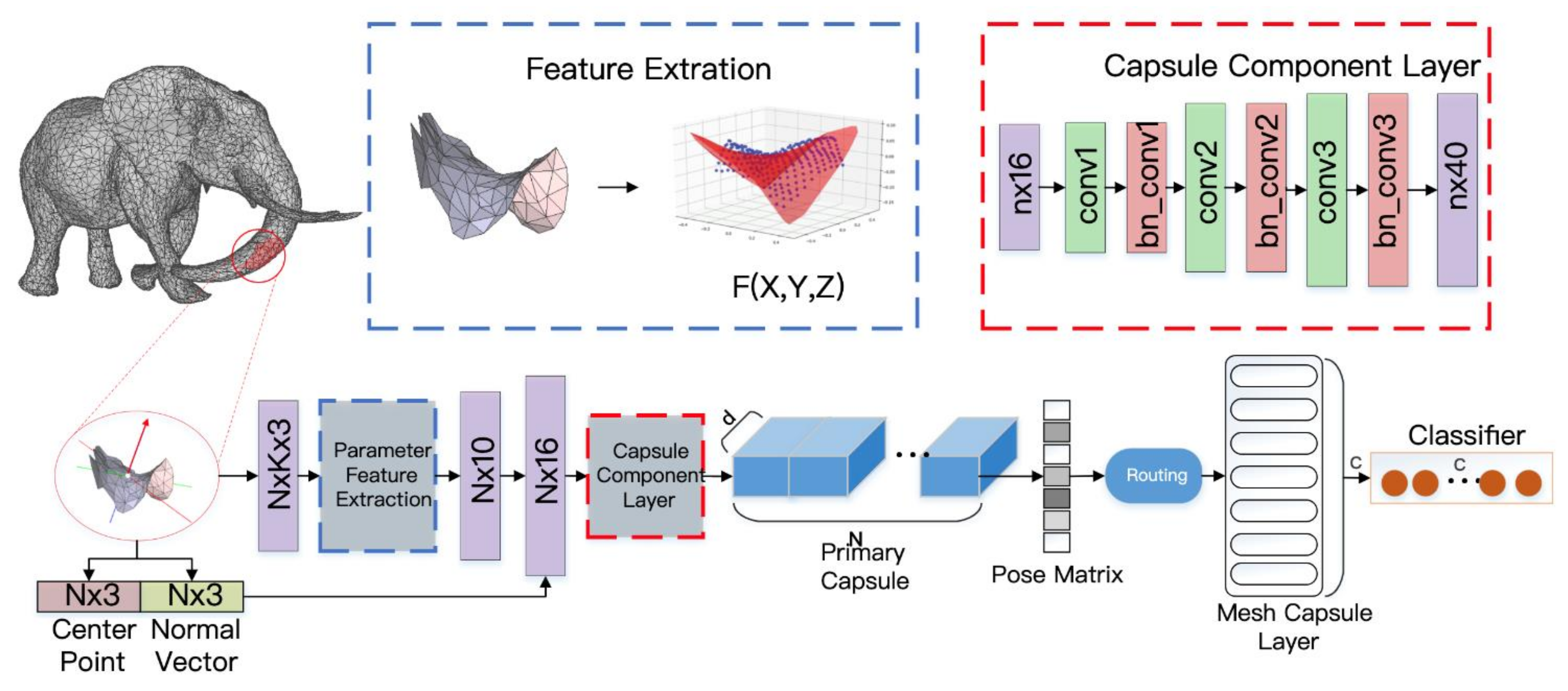
3.1. MeshCaps Framwork
The MeshCaps network structure is shown in Figure 3, and the training is divided into two stages. (1) Convolution feature mapping stage: the polynomial template is used as a convolution kernel to perform feature extraction operations on the entire model, and finally the convolution feature map at this stage is generated. (2) The training phase of the capsule network: the capsule network is composed of a capsule composition layer, a primary capsule layer, and a Mesh capsule layer, and the final output is used for classification. Compared with the ordinary capsule network, MeshCaps adds a capsule composition layer to map polynomial parameter features to the primary capsule layer extracts more representative features; at the same time, weight sharing is used to train the pose transformation matrix between the capsule layers, which no longer depends on the size of the input model.
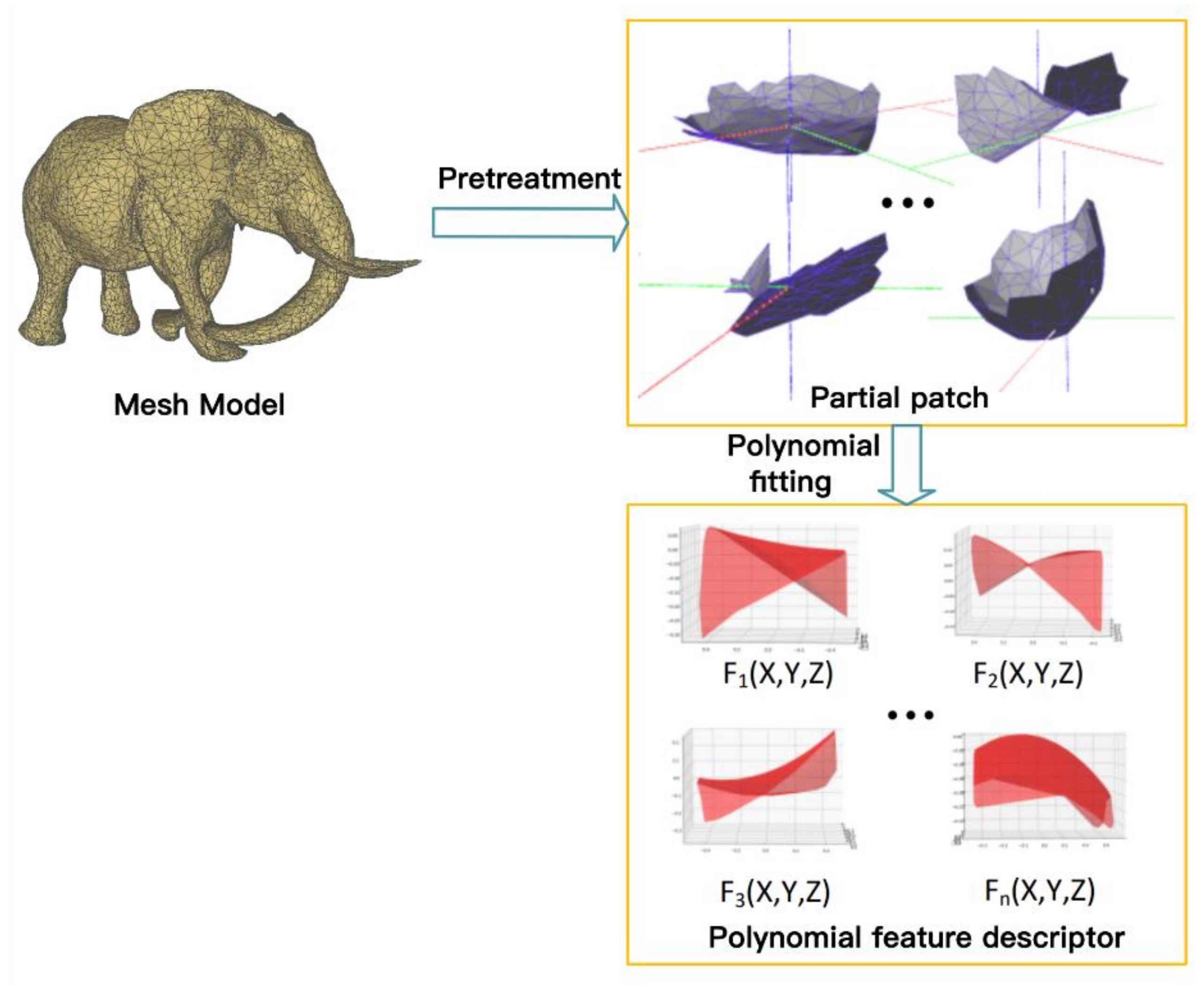
In the Figure 3, the box of feature extraction is the polynomial fitting of the surface element through the generalized least squares method(GLS), and the polynomial parameters are used as the surface features. For the convenience of comparison, the polynomial function F(X,Y,Z) is visualized in the feature extraction box of Figure 3. N represents the number of window surfaces, K represents the number of neighborhood points, N X 10 represents N surface elements, each surface is represented by a 10-dimensional high-order equation parameter, d represents the primary capsule dimension, and c represents the number of categories.
3.2. Local Shape Feature Extraction
We try to apply a more concise and light weight feature extraction method to the network model. Given a three-dimensional deformation target mesh model M, The local surface window of the 3D mesh model is defined as taking the vertex of the mesh model as the center of the window, using breadth-first search to get the front K-1 Neighbor vertices, the selected vertex and the edge between the vertices form a connected local mesh surface, that is, a local surface window , where:
K is the size of the convolution template window. For the selection of the k value, multiple sets of experiments have been carried out, and the best k value is 152, that is, the size of the convolution window is 152.
In order to avoid the influence of rigid transformation and nonrigid transformation, a local coordinate system is established in the window and the absolute coordinates of the vertices in the window are converted to the coordinate representation in the local coordinate system. Considering that the local surface in the window is relatively simple, the local coordinates in the window the system uses high-order polynomial equations to describe its shape, such as Formula (3):
where F is a continuous function used to describe the shape of the local grid window. is the parameter representation function of the grid. , and are the coordinates of the vertices in the window in the local coordinate system.
During the experiment, it was found that when the local window size is set very small, the grid shape is basically the same, and when K increases, the grid in the window becomes more complicated. Only the local m coordinate information of the vertex, , , is not enough to describe the grid shape. Therefore, we want to introduce the geodesic distance to improve the expression of a polynomial function. However, the calculation of the geodesic distance is a time-consuming operation, which affects the performance of the entire network, so the block distance is used as an approximate expression of the geodesic distance.
Among them, the block distance of a point in the convolution window is expressed as the block distance between the point and the center point of the surface unit.
For a grid window, assuming the relative coordinates of the vertices in the window , the window fitting function is as Formula (5):
The window fitting function , which is a continuous function used to describe the shape of the local window. Encode the local triangle set information, describe the local shape of the patch, and capture the shape transformation of the grid window. is the parameter representation of the grid. Where x, y, z, d represent , is the z in the formula, which is the z-axis coordinate of the point on the grid, which is used to measure the fitting error. The entire function F after fitting can be used as an approximate representation of the local grid.
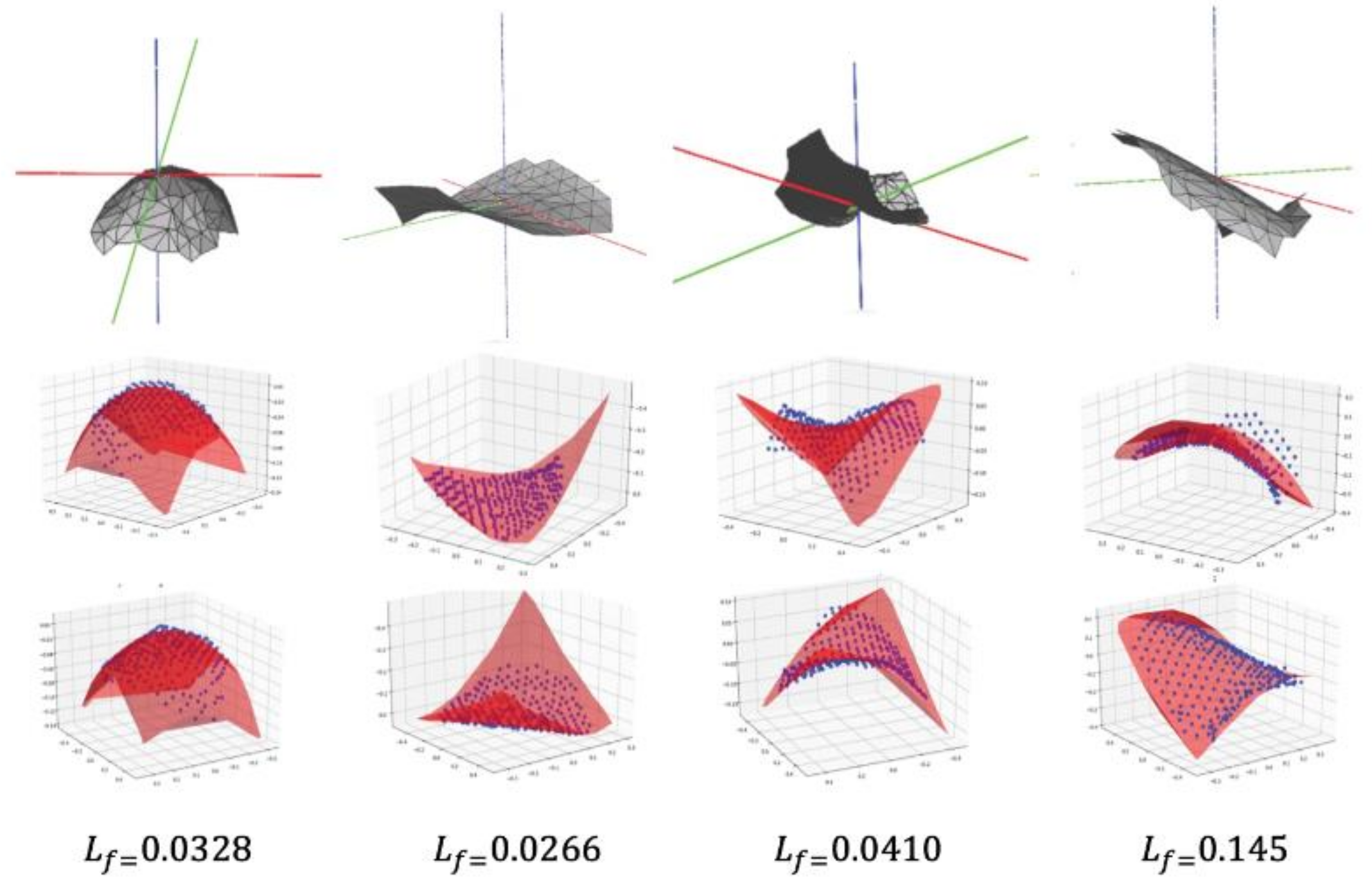
The surface fitting results are shown in Figure 4. The blue scatter plot represents the distribution of vertices in the grid window, and the red surface represents the result of fitting using a polynomial function. The fitting error is the mean error of all vertices of the surface.
In the fitting process, in order to avoid the influence of different positions and postures of the surface on the feature layer, the mesh is first positively definite. The center point is aligned with the origin of the three-dimensional coordinate system, and the normal vector is horizontal to the z-axis of the three-dimensional coordinate system. The equation parameters are solved by the generalized least squares method (GLS).
It can be seen from Figure 5 that each model can be represented by n parameter equations after sliding convolution through the window, and the parameters can be used as the shape feature descriptor of a certain mesh fragment under the window. At the same time, in order to introduce the surface pose information, after extracting the shape features of the mesh surface, the coordinates of the center point and the normal vector of the surface are added, so that the network can learn the direction information of the surface.
3.3. Mesh Capsule Networks
The traditional capsule network first uses the convolutional layer for feature extraction, and then gradually integrates it into deeper features through the capsule layer and uses them for classification results. However, because the result of feature extraction in the previous article is a shallow feature, certain spatial information is retained, and contains less semantic information, so after the feature extraction module, a capsule composition layer is added to map the equation parameter feature vector output to the primary capsule layer. For the convolutional feature layer, each patch is represented as a 10 polynomial of dimensional parameters. Through three one-dimensional convolutions, the number of channels is continuously increased to extract features of higher dimensions, and at the same time, each convolution uses a normalization layer to speed up the training and convergence of the network.
As shown in Figure 3, the primary capsule layer has N capsules, and each capsule has a dimension of d. The capsule composition layer maps feature vectors to the primary capsule layer , The capsules of each primary capsule layer are expressed as:
As a measure of the significant degree of a vector feature, the capsule network is normalized by a compression function. The capsule value is mapped to the [0,1] range, so that the length of the capsule vector can represent the probability of this feature, while preserving the eigenvalues of each dimension in the vector.
v is the output vector of the capsule, and S is the input vector of the capsule. Therefore, in order to calculate the output of each primary capsule, the activation function is applied.
Among them is the output of primary capsule.
Because the three-dimensional mesh model data set is different from the two-dimensional image, the size and size of each model are different in the input dimension, so an improvement has been made in the capsule network is changing the posture matrix between the bottom-level capsule and the high-level capsule in the network to the posture matrix with shared weights The training parameters are reduced, and because the pose matrix is changed from M × N to M × 1, the network can adapt to the input of three-dimensional models of different sizes. After all input vectors are mapped through the same pose matrix, the clustering results are output. Its expression is as follows:
is the output vector of the primary capsule layer, which is the pose matrix in the primary capsule layer, trained by the backpropagation algorithm.
The input of the Mesh capsule layer is the weighted sum of all capsule prediction vectors in the primary capsule layer.
where is the coupling coefficient that determines the similarity between and in the dynamic routing algorithm.
The initial logarithm is the log prior probability that capsule i should be coupled with capsule j. The dynamic routing algorithm of MeshCaps is the same as the routing algorithm in the original formula.
MeshCaps is only applied to three-dimensional mesh classification, so the reconstruction module and reconstruction loss in the traditional capsule network are discarded in the training and prediction process, which reduces the complexity of the model and helps improve the training efficiency of the model. Such as the formula:
Among them, c is the category, and is the indicator function of the classification. If the category c is correctly predicted, is equal to 1, otherwise it is 0. as the upper bound, that is, it is predicted that the category c exists but does not exist and the recognition is wrong. is the lower bound, that is, it is predicted that class c does not exist but does exist, and it is not recognized. λ is the proportional coefficient, adjust the proportion of the two. The parameter settings are as follows: . The total margin loss is calculated by summing the individual margin loss for all C classes.
4. Experimental Evaluation
To verify the effectiveness of the method, we validated it on the standard 3D deformable mesh model dataset SHREC15. The experimental computer was configured as an Intel (R) Xeon (R) processor with 64 GB memory. The SHREC15 dataset includes 50 categories, 1200 3D mesh models, and 24 models for each class. Each type of model has rigid transformation and nonrigid transformation. When training the classifier, 20 3D models were randomly selected for each class as training samples, and the rest were selected as test samples.
4.1. Model Details
The experiment was based on the Pytorch framework design. The model first passed the feature extraction module, traversed the points in the model, and took the convolution window with vertex as the center, and the size of the surface is 152. The polynomial parameters of the convolution were passed through the capsule composition layer, from three 20-dimensional, 30-dimensional, and 40-dimensional convolution layers. It then passed through the capsule dimension and the 40-input capsule layer, where the number of capsules was 50. The output capsule layer obtained a capsule size of 16 as the final classification output. The final length of each capsule was taken as the probability of the model belonging to the class. The learning rate of the whole network training period was not less than 0.001, and the batch size was 10. The accelerated calculation was carried out using a GPU, and the total training time was 2158 s.
4.2. Accuracy Test
In order to compare the superiority of the classification performance of the proposed method, this paper compares the traditional manual feature-based classification method SPH [28] and MeshNet [10], MeshCNN [9] by directly applying deep learning to the new method of three-dimensional grid classification. Table 1 shows for the classification results and average accuracy of the different categories of the data set.
Through experiments on different methods, it can be seen from Table 1 that the classification performance of the MeshCaps algorithm proposed in this paper was higher than other comparison methods. On the SHREC15 data set, the average accuracy rate reached 93.8%, which is comparable to the best results of the comparison method. In comparison, the average accuracy of the proposed method improved by 2.1% on the SHREC15 dataset. The experimental results show that the proposed 3D grid classification method based on the capsule network can obtain better results in the classification of 3D grid data.
In order to further prove the effectiveness of the proposed method and compare the convergence performance of different methods, it can be intuitively observed from the curve in Figure 6 that the MeshCaps method had good convergence. In the 15th round of iteration, the accuracy rate reached 86.63% and the convergence was reached earlier. The inflection point and the final convergence point prove that the dynamic routing in the capsule network performed unsupervised clustering of vector features to make the entire network converge quickly.
Because there are too many categories in the SHREC15 dataset, only the confusion matrix of 13 categories is displayed. As can be seen from Figure 6, MeshCaps was able to recognize most models. However, there were also several types of models with low recognition rates, such as glasses. We guess that, due to the use of curved surface units, the tails of glasses were more similar to pliers, which caused the model to have a higher misrecognition rate when recognizing these two types of models.
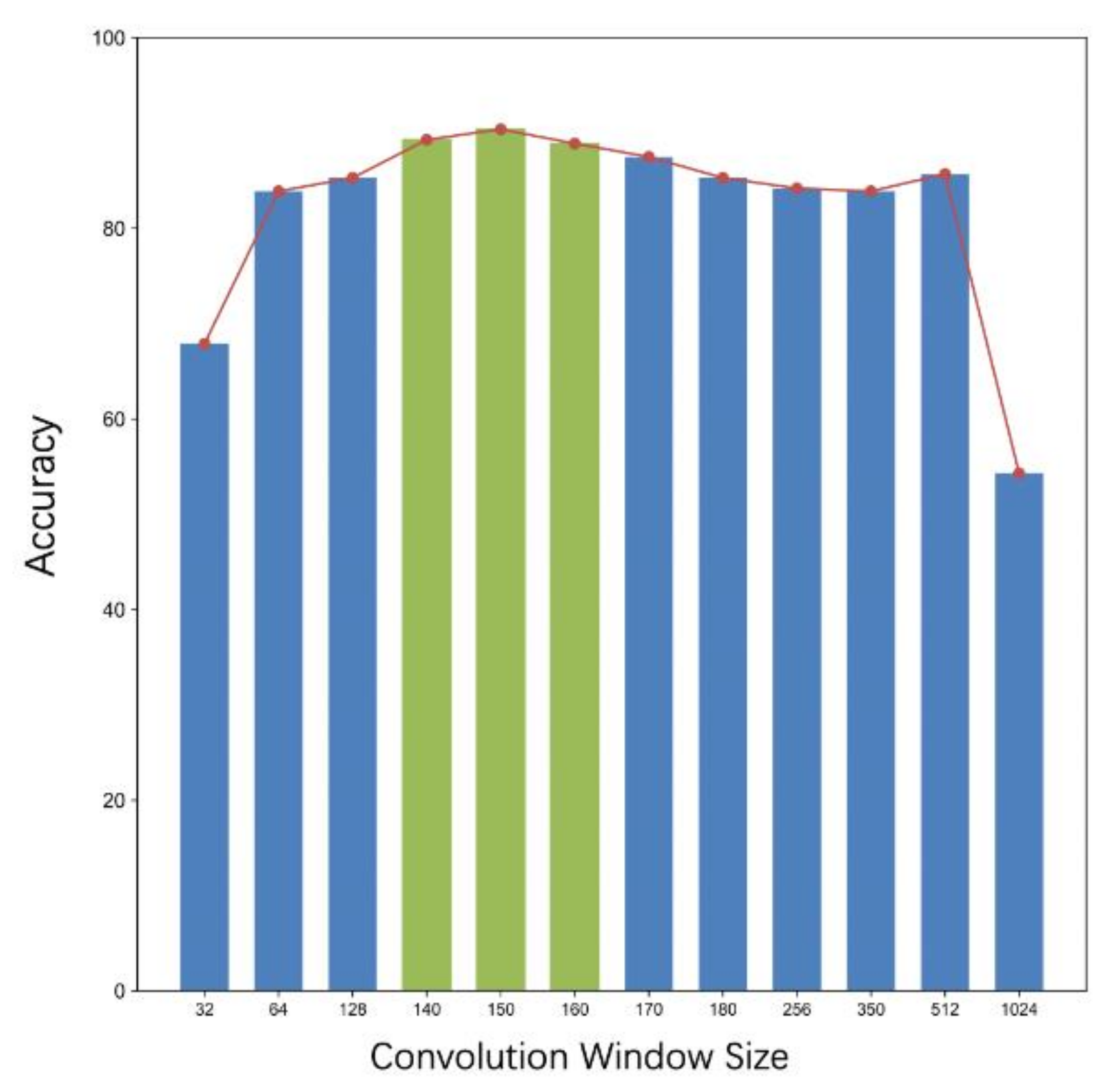
4.3. Convolution Window Size
In order to verify the optimal results produced by the different sizes of the convolution window in the proposed method, the convolution window was set to different sizes from 32 to 1024 for training. Figure 7 shows the window size, that is, the number of different neighborhood points taken as the calculation unit pair.
It can be seen from Figure 8 that under the premise that other parameters were fixed, the optimal convolution window size (shown in Table 2) was in the range of 140–160. When the window size was 32, 512, and 1024, the classification accuracy was 67.9%, 85.7%, and 54.3%, respectively. This is because when the local window size was set very small, the grid shape was basically the same, and the difference of various grids was too small, which affected the effect of feature clustering. When the convolution window was too large, the grid in the window changed to be even more complicated, increasing the network complexity and the amount of parameters, making the network easy to overfit. Experiments on the window size in this range, due to the different order of points of different data sets and for the SHREC15 data set, an average of 9000 points was experimentally verified convolution the optimal value of the window size is 152, that is, when 151 points around the vertex were taken as a calculation window according to the breadth-first search, the classification accuracy was the highest, and the classification accuracy reached 93.8%.
4.4. Model Complexity Comparison
Table 3 compares the time and space complexity of the network with other representative methods based on classification tasks. The column labeled #params shows the total number of parameters in the network, and the column labeled FLOPs/sample shows the input for each input the number of floating-point operations performed by the sample represents the space and time complexity. Among them, because the capsule network uses dynamic routing multiple iterations for feature clustering, the number of operations was higher, but it also made the entire network able to converge quickly. As shown in Figure 7, only a few iterations of training can achieve high accuracy.
4.5. Influencing Factor Experiment
In MeshCaps, there are two modules. In order to verify the effectiveness of feature fusion in the feature extraction module and the effectiveness of the capsule network in the classification module, the capsule network was replaced with a three-layer convolutional neural network and LeNet for experiments. To compare the classification accuracy, Table 4 shows the classification accuracy of different structures.
In the case of using the same feature method, MeshCaps achieved an accuracy of 93.8% compared with different classification network models, which illustrates the superiority of MeshCaps in the classification task of the SHREC15 data set. For complex data and capsule network comparison, the multilayer CNN structure has certain advantages. Compared with MeshCaps, which directly classifies polynomial parameter features through a three-layer convolutional neural network, the average accuracy reached 89.9%, which is higher than the accuracy of SPH method 88.2%, and also proves the effectiveness of the feature extraction method.
Since the method in this paper is different from the MeshCNN and MeshNet network structures, there was no pooling operation in the network, and the vertices were directly selected according to the breadth-first search method to obtain the local surface as an input unit. Therefore, the method of random sampling of the vertices was simplified during training, and the sampling points were the quantities shown in Table 5.
Because a patch unit is composed of multiple points around a vertex, a too high sampling percentage will inevitably cause the phenomenon of overlap of the patches, which affects the entire network training, and a model with a too low sampling ratio is prone to underfitting. The total number of vertices in the random sampling model was selected to be 85 % of vertices as input.
In the network design, the center point coordinates, normal vectors and polynomial parameters were feature fused, and the capsule composition layer was added for feature mapping. Comparative experiments were done on the influence of the capsule composition layer and feature fusion. The results are shown in Table 6.
The average accuracy of MeshCaps classification without feature fusion and no capsule composition layer still reached 91.2%, which is higher than the results obtained by the convolutional neural network method, and proves the certain advantages of the capsule network for complex data models. After fusing the features, classification of the increase in accuracy illustrates the effectiveness of feature fusion, but it was lower than the accuracy of the capsule composition layer and the unfused features, which verifies the importance of the capsule composition layer in the entire network structure.
5. Conclusions
In this paper, a 3D mesh model recognition algorithm based on an improved capsule network is proposed. It applies convolution directly to irregular 3D mesh models, extracts grid feature parameters by polynomial fitting, adds a capsule composition layer, extracts higher level features, and improves the weight matrix of the capsule to adapt to the differences in the input sizes of different models. After training, the average recognition accuracy was 92.3% on the original test set. By comparing with the traditional CNN network, the effectiveness of the capsule network was verified. Additionally, in comparison with other deep learning methods based on the grid model, the advantages of the MeshCaps convergence speed were verified. In subsequent research, the network can be further developed for 3D mesh segmentation or combined with a grid generation algorithm to perform more computer vision tasks.
Author Contributions
Conceptualization, J.Z. and Y.C.; methodology, Y.Z. and C.T.; software, Y.Z.; validation, Y.Z. and Y.C.; formal analysis, J.Z.; investigation, J.Z.; resources, S.Y.; data curation, Y.Z; writing—original draft preparation, Y.Z.; writing—review and editing, Y.Z.; visualization, Y.Z. and S.Y.; supervision, J.Z.; project administration, J.Z.; funding acquisition, J.Z. All authors have read and agreed to the published version of the manuscript.
Funding
This research was Supported by the National Natural Science Foundation of China (No. 62071260) and the National Youth Foundation of China (No. 62006131) and the K. C. Wong Magna Fund in Ningbo University. (Corresponding author: Jieyu Zhao)
Data Availability Statement
Not applicable, the study does not report any data.
Conflicts of Interest
The authors declare no conflict of interest.
References
- Xie, Z.-G.; Wang, Y.-Q.; Dou, Y.; Xiong, Y. 3D feature learning via convolutional auto-encoder extreme learning machine. J. Comput. Aided Des. Comput. Graph. 2015, 27, 2058–2064. (In Chinese) [Google Scholar]
- Wu, Z.; Song, S.; Khosla, A.; Yu, F.; Zhang, L.; Tang, X.; Xiao, J. 3d shapenets: A deep representation for volumetric shapes. In Proceedings of the IEEE Conference on Computer Vision and Pattern Recognition, Boston, MA, USA, 7–12 June 2015. [Google Scholar]
- Maturana, D.; Scherer, S. Voxnet: A 3d convolutional neu-ral network for real-time object recognition. In Proceedings of the Intelligent Robots and Systems (IROS), 2015 IEEE/RSJ International Conference on, Hamburg, Germany, 28 September–3 October 2015; pp. 922–928. [Google Scholar]
- Li, Y.; Pirk, S.; Su, H.; Qi, C.R.; Guibas, L.J. FPNN: Field probing neural networks for 3D data. In Proceedings of the Advances in Neural Information Processing Systems, Barcelona, Spain, 5–10 December 2016; pp. 307–315. [Google Scholar]
- Wang, D.Z.; Posner, I. Voting for voting in online point cloud object detection. In Proceedings of the Robotics: Science and Systems, Rome, Italy, 13–17 July 2015; p. 1317. [Google Scholar]
- Wang, P.; Liu, Y.; Guo, Y.-X.; Sun, C.-Y.; Tong, X. O-CNN: Octree-based Convolutional Neural Networks for 3D Shape Analysis. ACM Trans. Graph. 2017, 36, 11. [Google Scholar] [CrossRef]
- Qi, C.R.; Su, H.; Mo, K.; Guibas, L.J. Pointnet: Deep learning on point sets for 3D classification and segmentation. In Proceedings of the IEEE Conference on Computer Vision and Pattern Recognition, Honolulu, HI, USA, 21–26 July 2017. [Google Scholar]
- Qi, C.R.; Yi, L.; Su, H.; Guibas, L.J. Pointnet++: Deep hierarchical. feature learning on point sets in a metric space. Advances in Neural Information Processing Systems. arXiv 2017, arXiv:1706.02413. [Google Scholar]
- Hanocka, R.; Hertz, A.; Fish, N.; Giryes, R.; Fleishman, S.; Cohen-Or, D. MeshCNN: A network with an edge. ACM Trans. Graph. 2019, 38, 1–90. [Google Scholar] [CrossRef] [Green Version]
- Feng, Y.; You, H.; Zhao, X.; Gao, Y. MeshNet: Mesh. Neural Network for 3D Shape Representation. arXiv 2019, arXiv:1811.11424. [Google Scholar] [CrossRef]
- Yang, Y.; Liu, S.; Pan, H.; Liu, Y.; Tong, X. PFCNN: Convolutional Neural Networks on 3D Surfaces Using Parallel Frames. In Proceedings of the IEEE Conference on Computer Vision and Pattern Recognition, Online, 14, 15, 19 June 2020. [Google Scholar]
- Wang, J.; Wen, C.; Fu, Y.; Lin, H.; Zou, T.; Xue, X.; Zhang, Y. Neural Pose Transfer by Spatially Adaptive Instance Normalization. In Proceedings of the IEEE/CVF Conference on Computer Vision and Pattern Recognition, Seattle, WA, USA, 14–19 June 2020; pp. 5831–5839. [Google Scholar]
- Qiao, Y.L.; Gao, L.; Rosin, P.; Lai, Y.K.; Chen, X. Learning on 3D Meshes with Laplacian Encoding and Pooling. IEEE Trans. Vis. Comput. Graph. 2020. [Google Scholar] [CrossRef] [PubMed]
- Litany, O.; Bronstein, A.; Bronstein, M.; Makadia, A. Deformable shape completion with graph convolutional autoencod-ers. In Proceedings of the IEEE Conference on Computer Vision and Pattern Recognition, Salt Lake City, UT, USA, 18–22 June 2018; pp. 1886–1895. [Google Scholar]
- Zhang, X.; Luo, P.; Hu, X.; Wang, J.; Zhou, J. Research on Classification Performance of Small-Scale Dataset Based on Capsule Network. In Proceedings of the 2018 4th International Conference on Robotics and Artificial Intelligence (ICRAI 2018), Guangzhou, China, 17–19 November 2018; pp. 24–28. [Google Scholar] [CrossRef]
- Sabour, S.; Frosst, N.; Hinton, G.E. Dynamic routing be-tween capsules. In Proceedings of the Neural Information Processing Systems (NIPS), Long Beach, CA, USA, 4–9 December 2017. [Google Scholar]
- Hinton, G.E.; Krizhevsky, A.; Wang, S.D. Transforming auto-encoders. In Proceedings of the International Conference on Artificial Neural Networks (ICANN), Espoo, Finland, 14–17 June 2011; Springer: Berlin/Heidelberg, Germany, 2011. [Google Scholar]
- Ren, H.; Su, J.; Lu, H. Evaluating Generalization Ability of Convo-lutional Neural Networks and Capsule Networks for Image Classification via Top-2 Classification. arXiv 2019, arXiv:1901.10112. [Google Scholar]
- Iesmantas, T.; Alzbutas, R. Convolutional capsule network for classification of breast cancer histology images. In International Conference Image Analysis and Recognition (ICIAR); Springer: Berlin/Heidelberg, Germany, 2018; pp. 853–860. [Google Scholar]
- Jaiswal, A.; Abdalmageed, W.; Wu, Y.; Natarajan, P. Capsulegan: Generative adversarial capsule network. In Proceedings of the European Conference on Computer Vision (ECCV), Munich, Germany, 8–14 September 2018. [Google Scholar]
- Yang, M.; Zhao, W.; Ye, J.; Lei, Z.; Zhao, Z.; Zhang, S. Investigating capsule networks with dynamic routing for text classi-fication. In Proceedings of the Conference on Empirical Methods in Natural Language Processing (EMNLP), Brussels, Belgium, 31 October–4 November 2018; pp. 3110–3119. [Google Scholar]
- Nguyen, H.H.; Yamagishi, J.; Echizen, I. Capsule-forensics: Using capsule networks to detect forged images and videos. In Proceedings of the International Conference on Acoustics, Speech and Signal Processing (ICASSP), Brighton, UK, 12–17 May 2019; pp. 2307–2311. [Google Scholar]
- Bazazian, D.; Nahata, D. DCG-Net: Dynamic Capsule Graph Convolutional Network for Point Clouds. IEEE Access 2020, 8, 188056–188067. [Google Scholar] [CrossRef]
- Bazazian, D.; Parés, M. EDC-Net: Edge Detection Capsule Network for 3D Point Clouds. Appl. Sci. 2021, 11, 1833. [Google Scholar] [CrossRef]
- Zhao, Y.; Birdal, T.; Deng, H.; Tombari, F. 3D point capsule networks. In Proceedings of the IEEE/CVF Conference on Computer Vision and Pattern Recognition, Long Beach, CA, USA, 15–20 June 2019; pp. 1009–1018. [Google Scholar]
- Ahmad, A.; Kakillioglu, B.; Velipasalar, S. 3D capsule networks for object classification from 3D model data. In Proceedings of the 2018 52nd Asilomar Conference on Signals, Systems, and Computers, California, CA, USA, 28–31 October 2018; pp. 2225–2229. [Google Scholar]
- Lecun, Y.; Bottou, L. Gradient-based learning applied to doc-ument recognition. Proc. IEEE 1998, 86, 2278–2324. [Google Scholar] [CrossRef] [Green Version]
- Kazhdan, M.; Funkhouser, T.; Rusinkiewicz, S. Shape matching andanisotropy. ACM Trans. Graph. 2004, 23, 623–629. [Google Scholar] [CrossRef]
Figure 1.
The calculation process in a capsule.

Figure 2.
Capsule network and LeNet’s ability to classify rotating objects.

Figure 3.
Network framework.

Figure 4.
Mesh shape and second-order polynomial fitting.

Figure 5.
Polynomial feature extraction of mesh model.

Figure 6.
Convergence graph of each method.

Figure 7.
Convergence graph of each method.

Figure 8.
Convolution window size experiment.


Table 1.
SHREC15.
| Network | Alien | Ants | Cat | Dog1 | Hand | Man | Shark | Santa | Pliers | Glasses | Dog2 | Camel | Snake | Avg |
|---|---|---|---|---|---|---|---|---|---|---|---|---|---|---|
| SPH [28] | 87.4% | 86.2% | 90.4% | 89.3% | 88.6% | 89.1% | 90.2% | 89.4% | 87.1% | 89.9% | 86.7% | 88.1% | 87.9% | 88.2% |
| MeshNet [10] | 89.5% | 89.6% | 89.6% | 91.4% | 90.5% | 90.8% | 90.1% | 89.8% | 88.0% | 91.4% | 90.5% | 90.3% | 89.9% | 90.4% |
| MeshCNN [9] | 91.2% | 91.4% | 92.1% | 90.2% | 90.5% | 91.6% | 92.7% | 90.5% | 91.8% | 90.4% | 92.3% | 93.7% | 90.3% | 91.7% |
| Ours-MeshCaps | 92.7% | 91.2% | 91.9% | 92.4% | 94.2% | 92.8% | 93.0% | 92.9% | 94.1% | 90.2% | 95.3% | 92.3% | 95.0% | 93.8% |
Table 2.
Convolution window size.
| Window Size K | Acc |
|---|---|
| 140 | 89.3% |
| 142 | 91.8% |
| 144 | 91.6% |
| 146 | 92.2% |
| 148 | 92.9% |
| 150 | 93.0% |
| 151 | 93.3% |
| 152 | 93.8% |
| 153 | 93.5% |
| 154 | 92.8% |
| 156 | 93.0% |
| 158 | 92.2% |
| 160 | 91.9% |
Table 3.
Parameter comparison test.
| Network | Capacity (MB) | FLOPs/Sample (M) |
|---|---|---|
| MeshCNN [9] | 1.323 | 498 |
| MeshNet [10] | 4.251 | 509 |
| SPH [28] | 2.442 | 435 |
| Ours-MeshCaps | 3.342 | 605 |
Table 4.
Network structure comparison.
| Network Structure | Acc |
|---|---|
| Feature+3-Layer CNN | 89.9% |
| Feature+LeNet | 90.8% |
| MeshCaps | 93.8% |
Table 5.
Impact of sampling point.
| Sample Percentage | Acc |
|---|---|
| 100% | 87.4% |
| 95% | 85.8% |
| 90% | 91.8% |
| 85% | 93.8% |
| 80% | 89.5% |
| 75% | 79.1% |
| 70% | 80.4%% |
Table 6.
Feature fusion and composition layer influence experiment.
| Network Structure | Acc | |
|---|---|---|
| Component layer | Feature fusion | |
| No | No | 91.2% |
| No | Yes | 91.9% |
| Yes | No | 92.3% |
| Yes | Yes | 93.8% |
Publisher’s Note: MDPI stays neutral with regard to jurisdictional claims in published maps and institutional affiliations. |
© 2021 by the authors. Licensee MDPI, Basel, Switzerland. This article is an open access article distributed under the terms and conditions of the Creative Commons Attribution (CC BY) license (http://creativecommons.org/licenses/by/4.0/).
Share and Cite
MDPI and ACS Style
Zheng, Y.; Zhao, J.; Chen, Y.; Tang, C.; Yu, S. 3D Mesh Model Classification with a Capsule Network. Algorithms 2021, 14, 99. https://0-doi-org.brum.beds.ac.uk/10.3390/a14030099
AMA Style
Zheng Y, Zhao J, Chen Y, Tang C, Yu S. 3D Mesh Model Classification with a Capsule Network. Algorithms. 2021; 14(3):99. https://0-doi-org.brum.beds.ac.uk/10.3390/a14030099
Chicago/Turabian StyleZheng, Yang, Jieyu Zhao, Yu Chen, Chen Tang, and Shushi Yu. 2021. "3D Mesh Model Classification with a Capsule Network" Algorithms 14, no. 3: 99. https://0-doi-org.brum.beds.ac.uk/10.3390/a14030099
Note that from the first issue of 2016, this journal uses article numbers instead of page numbers. See further details here.