
Prediction of Intrinsically Disordered Proteins Using Machine Learning Algorithms Based on Fuzzy Entropy Feature

1
Tianjin Key Laboratory of Optoelectronic Sensor and Sensing Network Technology, School of Electronic Information and Optical Engineering, Nankai University, Tianjin 300350, China
2
Department of Communication Engineering, School of Electronic Information, Hebei University of Technology, Tianjin 300400, China
*
Author to whom correspondence should be addressed.
Algorithms 2021, 14(4), 102; https://0-doi-org.brum.beds.ac.uk/10.3390/a14040102
Submission received: 7 March 2021
/
Revised: 20 March 2021
/
Accepted: 21 March 2021
/
Published: 24 March 2021
(This article belongs to the Section Evolutionary Algorithms and Machine Learning)
Abstract
:We used fuzzy entropy as a feature to optimize the intrinsically disordered protein prediction scheme. The optimization scheme requires computing only five features for each residue of a protein sequence, that is, the Shannon entropy, topological entropy, and the weighted average values of two propensities. Notably, this is the first time that fuzzy entropy has been applied to the field of protein sequencing. In addition, we used three machine learning to examine the prediction results before and after optimization. The results show that the use of fuzzy entropy leads to an improvement in the performance of different algorithms, demonstrating the generality of its application. Finally, we compare the simulation results of our scheme with those of some existing schemes to demonstrate its effectiveness.
1. Introduction
Proteins play an important role as the main bearers of human life activities [1]. For a long time, the model of “lock and key” has been regarded as the general structural model of protein [2]. However, with the development of scientific research conditions, many proteins without fixed three-dimensional structure have been discovered by scientists [3]. Due to the lack of a fixed three-dimensional structure, the structural flexibility of these proteins makes them have the meaning that ordinary proteins do not have. With the discovery of more and more proteins without fixed structure, they have been identified as a large class of proteins, i.e., intrinsically disordered proteins. Recent studies have shown that innate intrinsically disordered proteins are widespread in organisms, and their proportions differ significantly between prokaryotes and eukaryotes [4]. Intrinsic disorder refers to segments or to whole proteins that fail to self-fold into fixed 3D structure, with such disorder sometimes existing in the native state [5]. The emergence of intrinsic disordered proteins has broken the unique functional pattern of proteins in the past, and because of their widespread existence in life, the research on them has become one of the topics widely discussed in recent years. In the past few decades, many methods have been developed to predict IDPs. Generally speaking, these methods can be divided into two categories: physicochemical-based and calculation-based. The first method is about employing the amino acid propensity scales and physicochemical properties of the protein sequences to predict IDPs, such as GlobPlot [6], IUPred [7], FoldUnfold [8] and IsUnstruct [9]. In the second method, the prediction of intrinsically disordered proteins is regarded as a binary classification problem and solved by machine learning. At present, many mature methods have been applied to IDPs prediction, such as Support Vector Machines, Convolutional Neural Network, long short term memory and so on. PONRD [10] is the first known mature machine learning algorithm for predicting intrinsically disordered proteins. It mainly uses neural network algorithm to distinguish amino acids by the different components of ordered and disordered amino acids. POODLE series of algorithms include POODLE-S [11], POODLE-L [12] and POODLEW [13] algorithms. They predicted regions with lengths less than 40, greater than 40, and overall disorder. Because of some differences in the structure of their prediction targets, their feature selection is slightly different. In addition, ESpritz [14] algorithm is also a relatively successful algorithm. Espritz can reduce the number of parameters and extract the hidden information from the sequence by recursive dynamic learning context. In addition to the conventional machine learning algorithm, the comprehensive prediction method based on a variety of independent prediction algorithms also shows good results in the prediction of intrinsically disordered proteins. The method is to run several independent intrinsically disordered protein prediction algorithms, and then get the final result through comprehensive prediction. Metadisorder is a very accurate algorithm. It includes 13 kinds of algorithms: Globplot, IUPred, DisEMBL, RONN, POODLES, DISPRED2 [15], DISPI [16], IPDA [17], PDISORDER [18], POODLE-L, PRDOS [19], Spritz [20], dispsmp [21]. The final results are weighted by these 13 algorithms, which have high accuracy. However, the efficiency of the algorithm is very low because it contains 13 independent prediction algorithms. In comparison, MFDP [22] with only three independent prediction algorithms is a relatively simple model. It integrates the results of IUPred, DISOPRED2, DISOclust [23] algorithms into SVM with linear kernel to get the final prediction.
Most current machine learning methods for intrinsically disordered protein prediction require as many as tens of features and have high computational complexity; they are less efficient when dealing with large amounts of data. We propose a new feature scheme based on fuzzy entropy; and test the feasibility of the scheme using three machine learning algorithms. Our scheme is trained and tested by the dataset DIS1616 with 10-fold cross-validation, firstly. The dataset DIS1616 is comprised of 1616 protein sequences with 2503 disordered regions and 2629 ordered regions, which include 186,069 disordered and 715,619 ordered residues. As a comparison, we run our schemes together with some existing schemes, such as DISOPRED2, RONN [24], DISPSSMP [25], Espritz and IsUnstructure [9] on the datasets R80 which are comprised of 78 protein sequences which include 2439 disordered and 19,412 ordered residues. The simulation results suggest that our scheme is at least as accurate as DiISPSSMP and requires computing only five features for each residue of a protein sequence, while the other need to compute 120 features for each residue, respectively.
In addition, we also compared the prediction performance of our algorithms before and after adding the fuzzy entropy feature; the results showed that the accuracy and stability of the predictions of our three selected algorithms improved after adding fuzzy entropy; according to the experimental results, the MCC values of the three algorithms improved by 4.22%, 3.92% and 9.09% respectively. This indicates that the addition of fuzzy entropy has a positive effect on the prediction of intrinsically disordered proteins and provides a new alternative method for protein prediction.
2. Features Selection of IDPS
In protein sequences, the sequence complexity indicates how many different rearrangements the sequence can have. Regions with low complexity are more likely to be disordered than regions with high complexity. Shannon entropy and topological entropy can reflect the complexity of protein sequences and have been used to relatively good effect in the prediction of intrinsically disordered proteins. Whereas fuzzy entropy is a concept first used in information theory to describe the degree of uncertainty of a probability distribution, it also indicates the complexity of the data. In this paper, it is used in intrinsically disordered protein sequencing and the feasibility of its application will be explored below. In this section, however, let us first briefly review the specific mathematical meaning of these features.
2.1. Shannon Entropy
For a given protein sequence, assuming its length to be n, the Shannon entropy can be calculated by the following equation:
In Formula (1), (1 ≤ k ≤ 20) represents the frequency of 20 amino acids in the sequence. The calculation formula is given in Formula (2):
In Formula (2), when J = k, K(j) = 1; otherwise K(j) = 0.
The corresponding values for the various amino acids used in the calculation of Shannon entropy are shown in Table 1:
2.2. Topological Entropy
In order to calculate the topological entropy, the complexity function (n) must be calculated first. It means the number of different subsequences with length n contained in the sequence w with length n (1 ≤ n ≤ N), which is calculated as shown in Equation (3):
In this formula, u is any continuous string of length N in the sequence w, and |u| = n means that the length of u is n. For example, given a sequence w = TASEAT, the subsequences of length 2 are:
{TA, AS, SE, EA, AT}
From this we can get (n) = 5.
If a protein sequence w with length n is given, the length n of its subsequence should satisfy the following formula:
20n + n − 1 ≤ |w| ≤ 20n + 1 + (n + 1) − 1
We use to represent the first sequence with length 20n + n − 1:
Then the topological entropy can be expressed as follows:
For the whole sequence, there are fragments with length . In order to improve the accuracy, we take the average value of each fragment as the final calculation result of topological entropy:
However, if the topological entropy is calculated according to the above equation, it is clear that the required sequence length would be very large, exceeding the sequence length of many proteins. Therefore, to facilitate the treatment of topological entropy for short sequences, we plot amino acid residues according to Table 1, and then the protein sequence becomes a 0–1 sequence, and the length of subsequence n can be given by the following equation:
2.3. Fuzzy Entropy
To better highlight the sequence complexity of proteins, we use fuzzy entropy as a new feature of protein sequences. This is the first time that fuzzy entropy has been used as a feature of a protein sequence in the study of an inherently disordered protein. For computational convenience, we use numbers from 0 to 19 to represent the 20 amino acids.
For {u(1), u(2) … U(N)}, the non-negative integer a is introduced to reconstruct the phase space, and the reconstructed sequence is:
And the membership fuzzy function is introduced:
According to the above formula, we can transform the fuzzy membership function into:
where is the distance between the window vectors , :
The corresponding values for each amino acid in the calculations are shown in Table 2:
So, we can get:
The fuzzy entropy of the sequence is:
In Equation (17), m, r, N represent the dimensionality of the phase space, the similarity tolerance and the length of the time series respectively. If M is too large, it will cause information loss, but too small will increase the sensitivity of the results to noise. According to the validation, the best experimental results were obtained when m = 2 or m = 3.
2.4. Amino Acid Propensity Scale
3. Algorithm Principle
There are many low-complexity intrinsically disordered protein-based algorithms, such as those constructed by He, H., Zhao, J. [26] and Liu, Y., Wang, X., Liu, B. [27] that have achieved good results. As the Disport dataset [28] we used to have a total of 1616 protein sequences and the training set contained a total of 900,000 amino acids, the sample size was large and the homology of the data was poor, some of the machine learning may not achieve the desired classification results. After preliminary research, LDA, SVM and BP neural networks are more suitable for low-complexity model building. And after experimental comparison and research, the three classification algorithms are more responsive to the differences between samples than other machine learning algorithms. Therefore, these three algorithms are chosen as the basis for this paper to verify the effectiveness of fuzzy entropy in inherently disordered protein prediction.
3.1. Linear Discriminant Analysis
LDA is mainly used in the field of pattern recognition. Recently, however, it has also performed well in the field of bioinformatics. Compared to some other learning methods, it is more purposeful and better reflects the differences between samples.
For a given characteristic matrix X = [, , … ], we use Ns to represent the number of samples, and , is used to represent the two kinds of discrimination. For the best projection direction W:
In this discrimination, we use Rayleigh entropy to reflect the classification effect. In order to calculate Rayleigh entropy, it is necessary to calculate the scattering matrix and scattering matrix :
The , in the above formula represents the expectations of the first and second types:
here, represents the set of samples of class i.
For the two species, we hope that the center distance of different species is as large as possible, while the data of the same kind after dimensionality reduction is as centralized as possible. Rayleigh entropy can well reflect these two properties:
The optimal projection direction can be obtained by using Lagrange operator:
Based on the optimal projection direction and true classification of each amino acid, a classification threshold ζ can be obtained, followed by the required classification plane.
3.2. Support Vector Machines
Support vector machines (SVM) is a binary classification model. Its purpose is to find a hyperplane to segment the sample. Its basic model is the linear classifier with the largest interval defined in the feature space 36.
For a given sample set, we need to find a hyperplane (W, b) so that the minimum geometric interval between the sample set and the hyperplane is the largest:
Equation (32) gives the formula for calculating the geometric interval. Our optimization goal is to maximize Formula (33) to obtain the optimal result. The formula is expressed as Formula (32):
Since the proportional scaling of w and b does not change the value of r, we add a constraint:
So optimization object becomes:
Then our final optimization goal is to:
We can use Lagrange multiplier method to transform the above formula into:
w and b in the original formula can be expressed by training samples and α:
where α is the Lagrangian multiplier and C is the penalty parameter. For the optimization in formula above, we use SMO algorithm. The principle of the algorithm is: change the minimum number of αi at a time. First we select , and hold other parameters unchanged. Then optimization object becomes the following form:
The results can be obtained by iterating until convergence.
3.3. Back Propagation Neural Network
BP neural network is a kind of multilayer feedforward network trained by error back propagation algorithm [29]. It has shown excellent performance in bioinformatics. In protein sequencing, BP neural networks play a good role in classification. Since BP neural networks are fully connected networks, each dimension of the space is affected by all dimensions of the source space, and the data is utilized to the fullest extent that classification results can be obtained very accurately. Below we will describe this network in brief terms.
In Formula (35), , i is the i-th line of parameter W[l] and A[l−1] is the output of layer L − 1.
Then, for the characteristic matrix X, the determination of each sample can be obtained according to Formulas (44) and (45):
After getting the prediction result of training samples, we use cross entropy to calculate the cost function of BP neural network:
where is the predicted value of each sample and is the true value of each sample.
In order to optimize the cost function, we use back propagation to train the optimization parameter , . The process of back propagation is as follows:
4. Performance Evaluation
In bioinformatics, sensitivity (Sens), specificity (Spec) and Matthews’ correlation coefficient (MCC) are often used to evaluate predictive outcomes. For example, in the study by Lee, Khanh [30] and in the study by Lam, Luu Ho Thanh [31], these three parameters were utilized to evaluate the model. On this basis, we have also chosen the weight score (Sw) for our algorithms as evaluation criteria. These evaluation measurements are defined as follows:
Sensitivity:
Specificity:
The weighted score:
Matthews’ correlation coefficient:
In the above formula, TP and TN are the predicted correct ordered and disordered amino acids, respectively; FP and FN are the mispredicted ordered and disordered amino acids, respectively.
5. Data Preprocessing Method
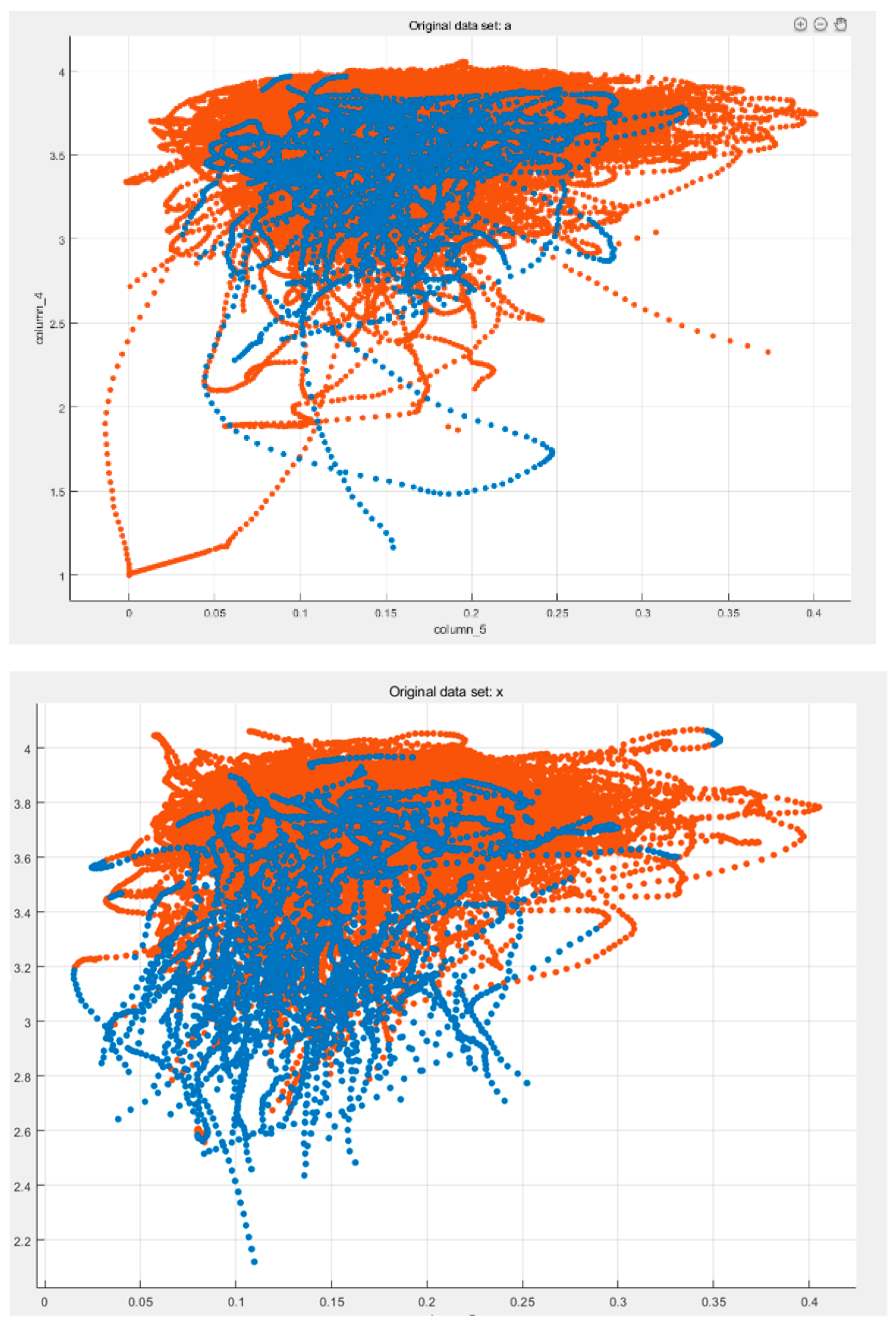
It is not ideal to directly calculate the characteristics of each amino acid and classify them. To make the results more accurate, we added a sliding window to pre-process the data. For a given protein sequence of length L, we need to choose a sliding window of length N and add [N/2] zeros to both ends of the sequence. For the region intercepted by the sliding window, a five-dimensional feature vector can be obtained for each amino acid in that region. The average of the eigenvectors of all amino acids in the sliding window is taken as the eigenvalue of each residue in the window. As the window slides, the eigenvalues for each amino acid are accumulated. Finally, the sum of the eigenvalues obtained for the amino acids is divided by the cumulative number. Each amino acid in the protein sequence is then given a five-dimensional eigenvector as the feature vector for that amino acid. The equation for this process is as follows.
Taking feature Bfactor(2STD) and fuzzy entropy as examples. After windowing, the separability of the two categories of data is significantly improved, and the effect is shown in Figure 1.
The accuracy as well as the stability of the prediction results of each learning method has been improved after the raw data has been processed by adding windows. We have compared the MCC values of different learning algorithms before and after windowing, using a window length of 35 as an example, and the comparison results are shown in Table 4.
6. Result and Discussion
6.1. The Simulation Results
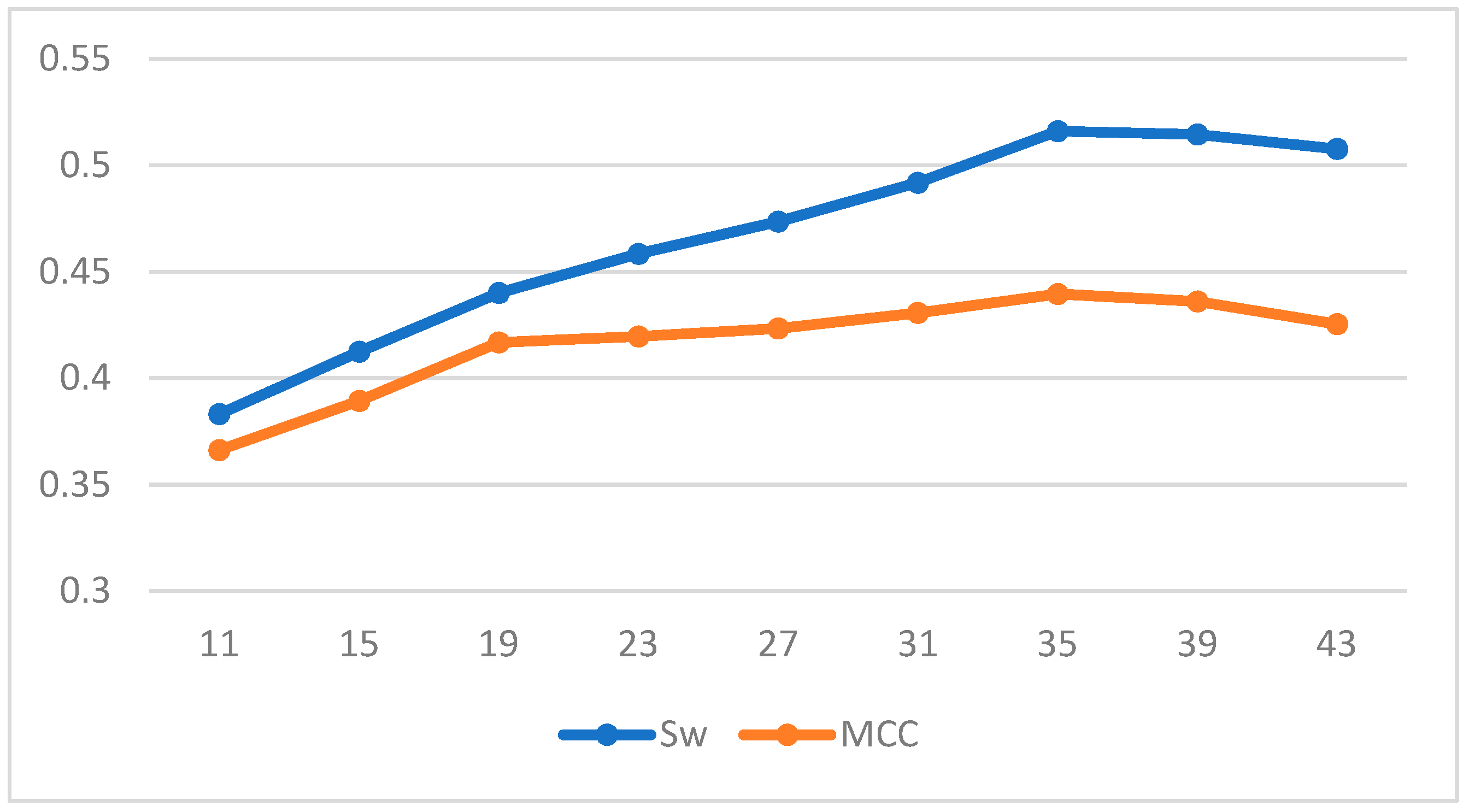
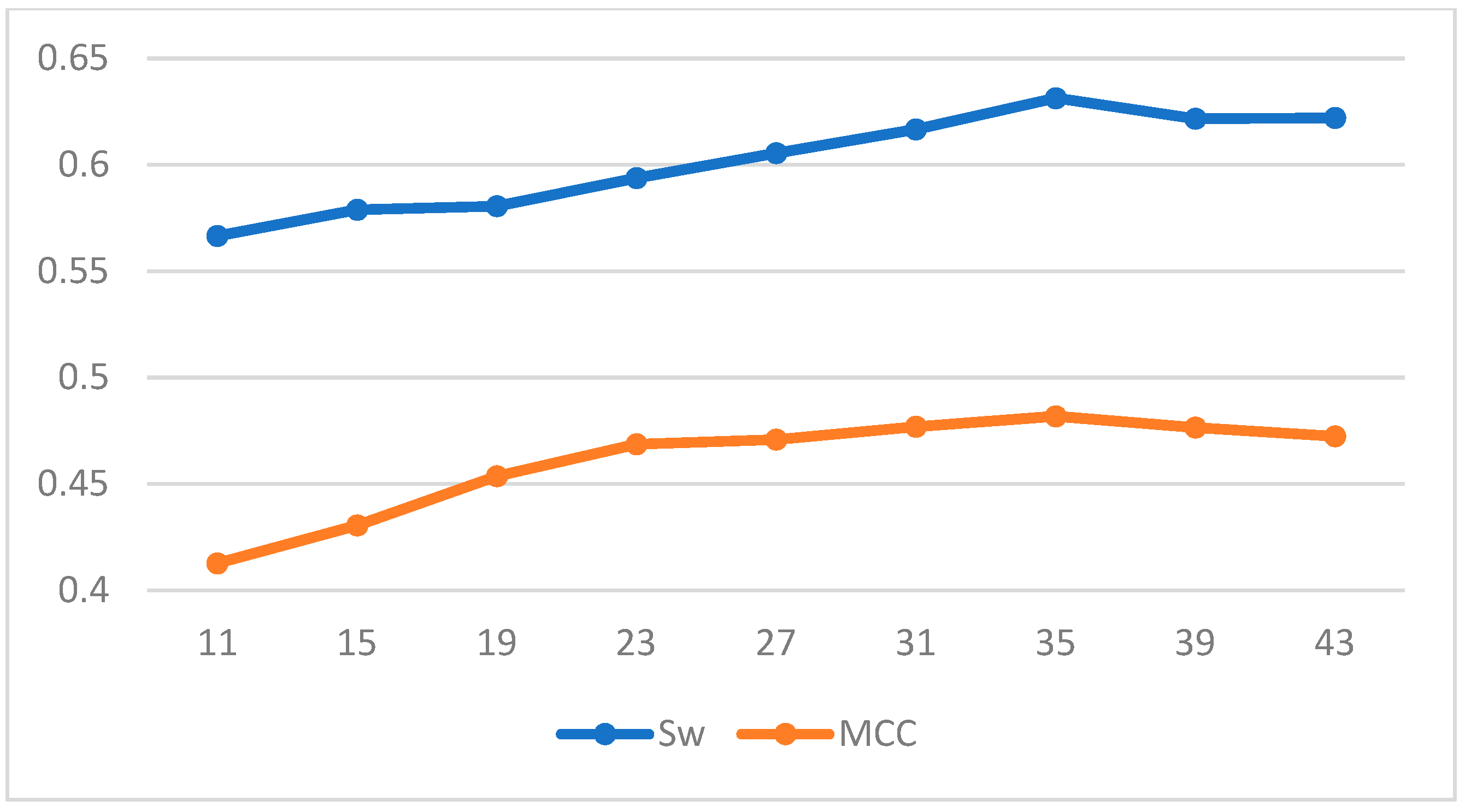
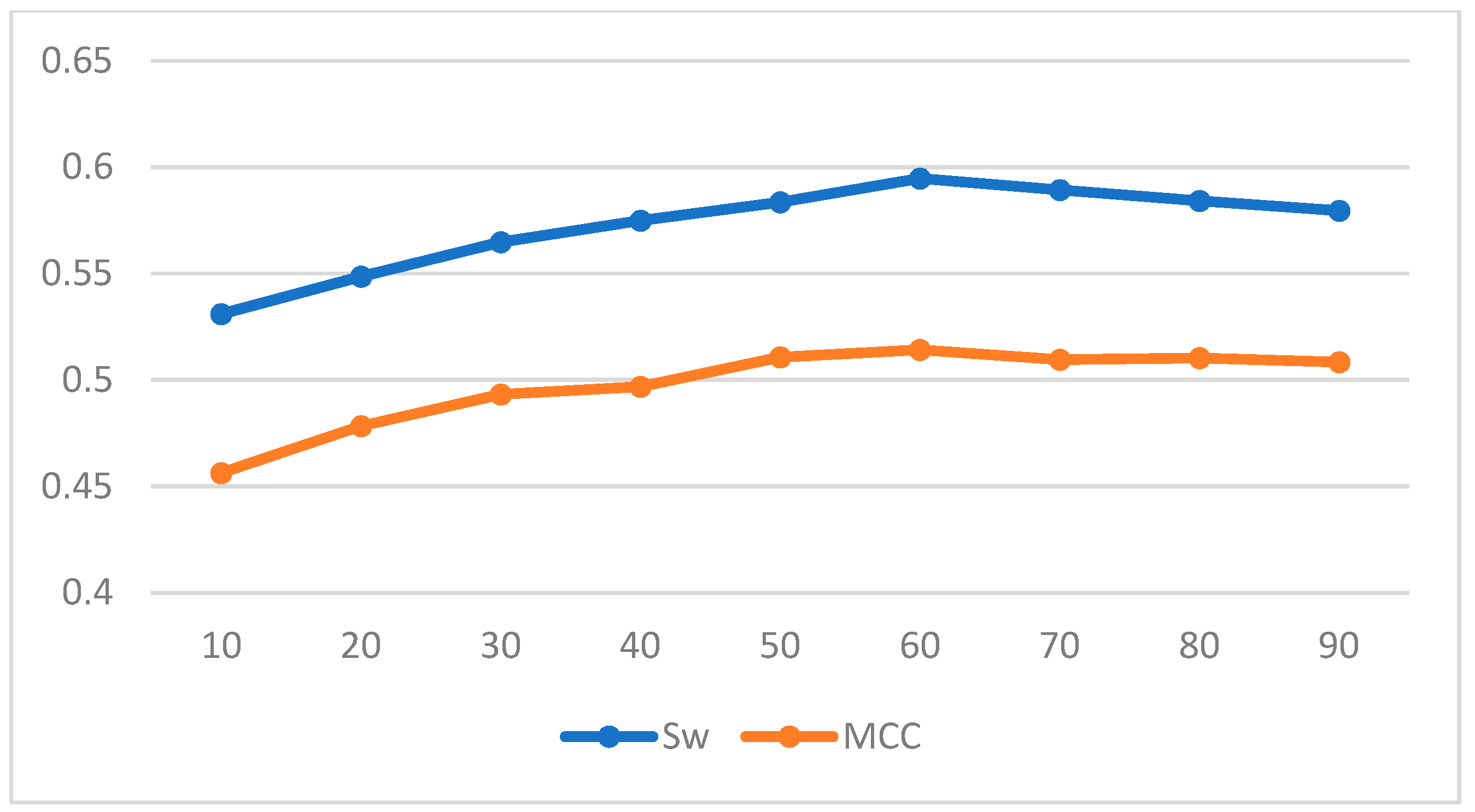
To train our prediction scheme, we randomly divided the 1616 protein sequences in Disport into ten subsets of approximately equal size and trained them using ten-fold cross-validation. The results of our three chosen machine learning methods under different windows are shown in the Table 5 and Table 6; and Figure 2, Figure 3 and Figure 4 plot the effect of different window lengths on the prediction performance of the three learning algorithms:
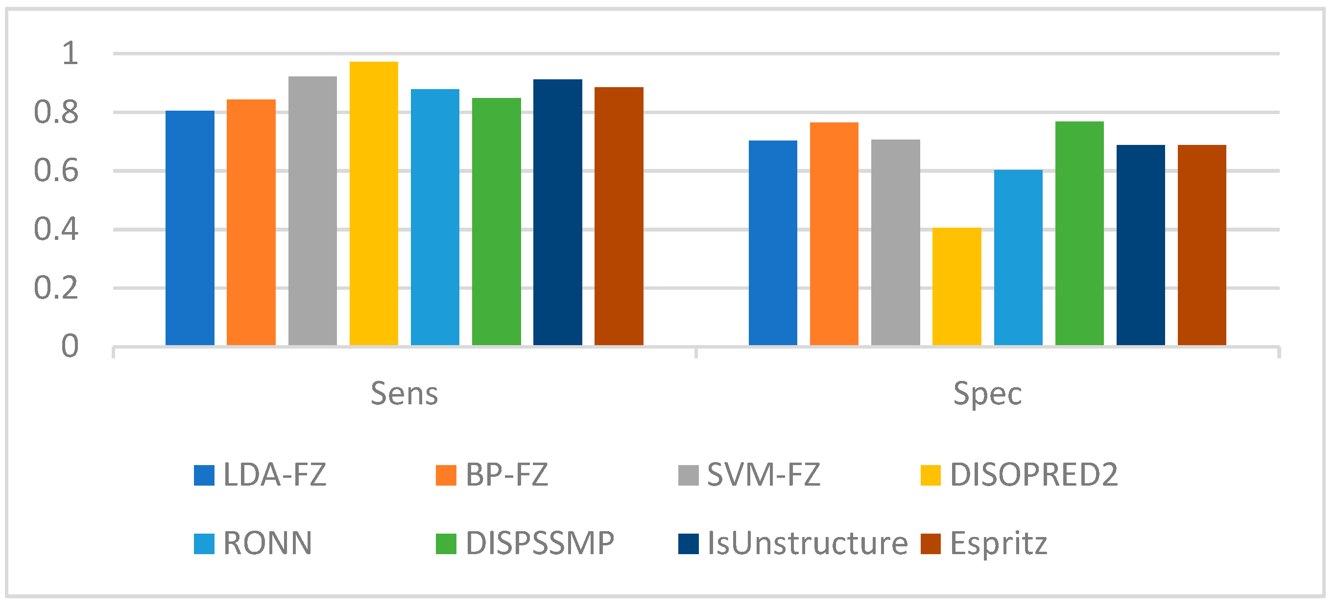
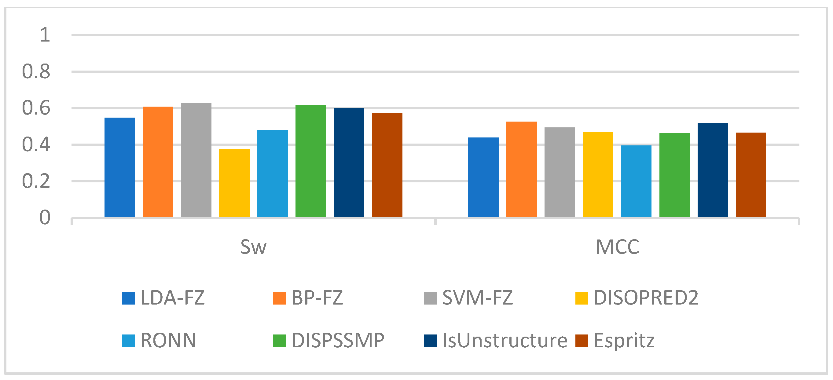
Using the data in the table we find that for LDA and SVM, when the window size is larger than 35, the values tend to be smooth; for BP neural networks, when the window size is larger than 60, the values tend to be smooth. Therefore, we use a window length of 35, 60 as the selection window length for the corresponding algorithm. As a comparison, we run our scheme together with some of the best-known schemes, such as Espritz [14], DISOPRED2 [15], RONN [24], DISPSSMP [25] and IsUnstructure [9] on the dataset R80 which are comprised of 78 protein sequences. Table 7 shows the prediction results of these learning methods on the test set; in Figure 5 and Figure 6 we have visualized these results to make the comparison between the different algorithms more intuitive.
Considering the classification method used, we use LDA-FE, SVM-FE, BP-FE as the abbreviation of our scheme. As shown in Table 6, the highest Sens, Spec, Sw, and MCC among all algorithms are DISOPRED2, DISPSSMP, SVM-FZ and BP-FE, respectively. Among all algorithms, only our BP-FE algorithm and IsUnstructure achieve 0.5 for MCC. Taking all parameters together, DISPSSMP, IsUnstructure and SVM-FZ, BP-FE are close to each other. However, our algorithms requires only five features of amino acids for classification, whereas other algorithms with similar results to ours, such as DISPSSMP and Espritz, require 188 and 25 features of each amino acid. Moreover, since our method has a simpler decision curve calculation, our solution is more robust and requires fewer learning samples than DISPSSMP, IsUnstructure, etc.
6.2. The Influence of Fuzzy Entropy on Prediction Effect
Since this paper introduces the feature of fuzzy entropy in the prediction process, it is necessary for us to explore whether fuzzy entropy has a positive effect in the prediction of inherently disordered proteins.
To ensure that fuzzy entropy plays an active role in the prediction of inherently disordered proteins, we compared three learning algorithms with and without the feature of fuzzy entropy, and the results of the comparison are shown in Table 8, Table 9 and Table 10.
By comparison, the values of SW and MCC improved for all three models we constructed after adding fuzzy entropy as a feature. In BP-FE, the most effective of the three algorithms, the addition of the fuzzy entropy feature improved the value of MCC by 9.09% and the accuracy of prediction from 84% to 88%. The MCC values for LDA-FE and SVM-FE also improved by 4.22% and 3.92% respectively. This shows that fuzzy entropy shows a positive effect in the prediction of inherently disordered proteins.
In order to compare the different models more intuitively, we conducted significance tests for the three models we used. We make the assumption that the two algorithms used as a comparison have the same performance. With this assumption we perform a significance test; their p-values against each other are shown in Table 11:
By calculating the p-value, we find that the p-value between LDA-FE and SVM-FE, BP-FE is much less than 0.05, so we can assume that the performance of LDA-FE is inferior to the latter two; while the p-value between SVM-FE, BP-FE is 0.1679, which is much greater than 0.05; therefore, according to SW as well as the MCC values, SVM-FE, BP-FE are equally good.
7. Conclusions
With the advent of the post-genetic era, the number of protein sequences of unknown structure and function has exploded. The advent of machine learning allows for efficient processing of these sequences. In this paper, machine learning algorithms are used to classify and identify intrinsically disordered proteins. The taxonomic identification of such proteins is the first and most important step in understanding their biological properties. In protein identification, feature extraction, which represents protein sequence information in numerical form, is an important step in the overall model construction. In recent years, a variety of feature extraction algorithms have been applied in bioinformatics research. Appropriate feature extraction algorithms can achieve twice the result with half the effort. The main research and the results achieved in this paper are summarized as follows:
- 1.
- In the sequence identification of intrinsically disordered proteins, this paper extracts feature sets based on topological entropy, Shannon entropy, fuzzy entropy and information from two amino acid propensity tables. The multiple perspectives of information extraction can lead to a better representation of the sequence information of proteins. Among them, fuzzy entropy is applied as a feature for the first time in this field.
- 2.
- In response to the uneven distribution of the dataset and the poor homogeneity of the dataset as a whole, we have used a windowing approach to the dataset. After comparison, the windowed data is more robust and has a more concentrated data distribution, and is more accurate for predicting inherently disordered proteins.
- 3.
- After comparison, the performance of all three algorithms we constructed was improved after applying fuzzy entropy as a feature. Moreover, the recognition accuracy of our algorithms is as accurate as several current algorithms. Among the three schemes we constructed, BP-FE performs the best, and the MCC can reach 0.51, which exceeds many existing schemes. It is worth noting that the algorithm that uses fuzzy entropy as a feature requires only five features, whereas most algorithms used as a comparison require more than 30 features to make predictions.
Overall, we provide a new way of thinking about feature selection for protein sequencing. However, due to the large number of knowledge points in the field of bioinformatics and the short period of time in which the relevant research has been conducted, there are certain shortcomings in the thesis. The following section summarizes the shortcomings of this research and the ideas for future research work:
- 1.
- Although this paper has achieved good results for the identification of intrinsically disordered proteins, a classification model with higher prediction accuracy and more practical significance is needed for practical applications. Therefore, in future studies on intrinsically disordered proteins, more in-depth studies will be carried out with the aim of further improving the MCC by considering more influencing factors as a condition. For example, amino acids possess more than 500 physicochemical properties, can these five features we have chosen contain information on all aspects of amino acids? This is a question that we need to focus on in our future work.
- 2.
- As classification of intrinsically disordered proteins is a more fundamental part of proteomics, deeper exploration is essential in order to take full advantage of the unique biological functions of each intrinsically disordered protein. Future research may revolve around exploring the interactions between intrinsically disordered proteins, protein-ligand interactions, etc.
Author Contributions
Conceptualization, H.L.; project administration, H.L.; supervision, H.L.; validation, H.L. and L.Z.; formal analysis, L.Z.; investigation, L.Z.; methodology, L.Z.; software, L.Z.; writing—original draft preparation, L.Z.; writing—review and editing, L.Z.; resources, H.H. All authors have read and agreed to the published version of the manuscript.
Funding
The authors received no specific funding for this study.
Data Availability Statement
Publicly available datasets were analyzed in this study. These data can be found on the website: https://disprot.org (accessed on 22 March 2021). and in the datasets provided in the published [9,14,15].
Acknowledgments
The authors are thankful for the support from Nankai University, School of Electronic Information and Optical Engineering.
Conflicts of Interest
The authors declare that they have no conflicts of interest to report regarding the present study.
References
- Nordberg, R.C.; Loboa, E.G. Our Fat Future: Translating Adipose Stem Cell Therapy. Stem Cells Transl. Med. 2015, 4, 974–979. [Google Scholar] [CrossRef]
- Lieutaud, P.; Ferron, F.; Uversky, A.V.; Kurgan, L.; Uversky, V.N.; Longhi, S. How disordered is my protein and what is its disorder for? A guide through the “dark side” of the protein universe. Intrinsically Disord. Proteins 2016, 4, e1259708. [Google Scholar] [CrossRef] [PubMed] [Green Version]
- Dunker, A.K.; Lawson, J.D.; Brown, C.J.; Williams, R.M.; Romero, P.; Oh, J.S.; Oldfield, C.J.; Campen, A.M.; Ratliff, C.M.; Hipps, K.W.; et al. Intrinsically disordered protein. J. Mol. Graph. Model. 2001, 19, 26–59. [Google Scholar] [CrossRef] [Green Version]
- Oldfield, C.J.; Dunker, A.K. Intrinsically Disordered Proteins and Intrinsically Disordered Protein Regions. Ann. Rev. Biochem. 2014, 83, 553–584. [Google Scholar] [CrossRef] [PubMed]
- Romero, P.; Obradovic, Z.; Li, X.; Garner, E.C.; Brown, C.J.; Dunker, A.K. Sequence Complexity of Disordered Protein. Proteins Struct. Funct. Bioinform. 2001, 42, 38–48. [Google Scholar] [CrossRef]
- Rune, L.; Russell, R.B.; Victor, N.; Gibson, T.J. GlobPlot: Exploring protein sequences for globularity and disorder. Nucleic Acids Res. 2003, 31, 3701–3708. [Google Scholar]
- Zsuzsanna, D.; Tompa, P.; Simon, I. Prediction of protein disorder at the domain level. Curr. Protein Peptide Sci. 2007, 8, 161–171. [Google Scholar]
- Jaime, P.; Felder, C.E.; Tzviya, Z.B.M.; Rydberg, E.H.; Man, O.; Beckmann, J.S.; Silman, I.; Sussman, J.L. FoldIndexl©: A simple tool to predict whether a given protein sequence is intrinsically unfolded. Bioinformatics 2005, 21, 3435–3438. [Google Scholar]
- Lobanov, M.Y.; Galzitskaya, O.V. The Ising model for prediction of disordered residues from protein sequence alone. Phys. Biol. 2011, 8, 035004. [Google Scholar] [CrossRef] [PubMed]
- PONDR: Predictors of Natural Disordered Regions. Available online: http://www.pondr.com/ (accessed on 12 June 2007).
- Shimizu, K.; Hirose, S.; Noguchi, T. POODLE-S: Web application for predicting protein disorder by using physicochemical features and reduced amino acid set of a position-specific scoring matrix. Bioinformatics 2007, 23, 2337. [Google Scholar] [CrossRef]
- Hirose, S.; Shimizu, K.; Kanai, S.; Kuroda, Y.; Noguchi, T. POODLE-L: A two-level SVM prediction system for reliably predicting long disordered regions. Bioinformatics 2007, 23, 2046–2053. [Google Scholar] [CrossRef] [PubMed] [Green Version]
- Shimizu, K.; Muraoka, Y.; Hirose, S.; Tomii, K.; Noguchi, T. Predicting mostly disordered proteins by using structure unknown protein data. BMC Bioinform. 2007, 8, 1–15. [Google Scholar] [CrossRef] [PubMed] [Green Version]
- Walsh, I.; Martin, A.J.; Di Domenico, T.; Tosatto, S.C.E. ESpritz: Accurate and fast prediction of protein disorder. Bioinformatics 2012, 28, 503–509. [Google Scholar] [CrossRef] [PubMed] [Green Version]
- Ward, J.J.; Mcguffin, L.J.; Bryson, K.; Buxton Bernard, F.; Jones, D.T. The DISOPRED server for the prediction of protein disorder. Bioinformatics 2004, 20, 2138–2139. [Google Scholar] [CrossRef]
- Medina, M.W.; Gao, F.; Naidoo, D.; Rudel, L.L.; Temel, R.E.; McDaniel, A.L.; Marshall, S.M.; Krauss, R.M. Coordinately Regulated Alternative Splicing of Genes Involved in Cholesterol Biosynthesis and Uptake. PLoS ONE 2011, 6, e19420. [Google Scholar] [CrossRef] [Green Version]
- Chung-Tsai, S.; Chien-Yu, C.; Chen-Ming, H. iPDA: Integrated protein disorder analyzer. Nucleic Acids Res. 2007, 35, 465–472. [Google Scholar]
- Tompa, M.F.P.; Simon, I. Local structural disorder imparts plasticity on linear motifs. Bioinformatics 2007, 23, 950–956. [Google Scholar]
- Ishida, T.; Kinoshita, K. PrDOS: Prediction of disordered protein regions from amino acid sequence. Nucleic Acids Res. 2007, 35, W460–W464. [Google Scholar] [CrossRef]
- Alessandro, V.; Oscar, B.; Gianluca, P.; Tosatto, S.C.E. Spritz: A server for the prediction of intrinsically disordered regions in protein sequences using kernel machines. Nucleic Acids Res. 2006, 34, 164–168. [Google Scholar]
- Su, C.T.; Chen, C.Y.; Ou, Y.Y. Protein disorder prediction by condensed PSSM considering propensity for order or disorder. BMC Bioinform. 2006, 7, 1–16. [Google Scholar] [CrossRef] [Green Version]
- Mizianty, M.J.; Stach, W.; Chen, K.; Kedarisetti, K.D.; Disfani, F.M.; Kurgan, L. Improved sequence-based prediction of disordered regions with multilayer fusion of multiple information sources. Bioinformatics 2010, 26, i489–i496. [Google Scholar] [CrossRef] [PubMed] [Green Version]
- Mcguffin, L.J. Intrinsic disorder prediction from the analysis of multiple protein fold recognition models. Bioinformatics 2008, 24, 1798–1804. [Google Scholar] [CrossRef] [Green Version]
- Yang, Z.R.; Thomson, R.; Mcneil, P.; Esnouf, R.M. RONN: The bio-basis function neural network technique applied to the detection of natively disordered regions in proteins. Bioinformatics 2005, 21, 3369–3376. [Google Scholar] [CrossRef] [PubMed] [Green Version]
- Kaya, I.E.; Ibrikci, T.; Ersoy, O.K. Prediction of disorder with new computational tool: BVDEA. Exp. Syst. Appl. 2011, 38, 14451–14459. [Google Scholar] [CrossRef] [Green Version]
- He, H.; Zhao, J. A Low Computational Complexity Scheme for the Prediction of Intrinsically Disordered Protein Regions. Math. Probl. Eng. 2018, 2018, 1–7. [Google Scholar] [CrossRef] [Green Version]
- Liu, Y.; Wang, X.; Liu, B. IDPCRF: Intrinsically Disordered Protein/Region Identification Based on Conditional Random Fields. Int. J. Mol. Sci. 2018, 19, 2483. [Google Scholar] [CrossRef] [Green Version]
- Megan, S.; Hamilton, J.A.; Tanguy, L.G.; Vacic, V.; Cortese, M.S.; Tantos, A.; Szabo, B.; Tompa, P.; Chen, J.; Uversky, V.N.; et al. DisProt: The Database of Disordered Proteins. Nucleic Acids Res. 2007, 35, 786–793. [Google Scholar]
- Wei, L.; Ding, Y.; Su, R.; Tang, J.; Zou, Q. Prediction of human protein subcellular localization using deep learning. J. Parallel Distrib. Comput. 2017, 117, 212–217. [Google Scholar] [CrossRef]
- Lee, K.; Do, D.T.; Hung, T.N.K.; Lam, L.H.T.; Huynh, T.; Nguyen, N.T.K. A Computational Framework Based on Ensemble Deep Neural Networks for Essential Genes Identification. Int. J. Mol. Sci. 2020, 21, 9070. [Google Scholar] [CrossRef]
- Lam, L.H.T.; Le, N.H.; van Tuan, L.; Tran Ban, H.; Nguyen Khanh Hung, T.; Nguyen, N.T.K.; Huu Dang, L.; Le, N.Q.K. Machine Learning Model for Identifying Antioxidant Proteins Using Features Calculated from Primary Sequences. Biology 2020, 9, 325. [Google Scholar]
Figure 1.
Bfactor(2STD)and fuzzy entropy before and after windowing.

Figure 2.
Effect of different window length on prediction performance of LDA.

Figure 3.
Effect of different window length on prediction performance of SVM.

Figure 4.
Effect of different window length on prediction performance of BP neural network.

Figure 5.
Prediction performance comparison based on test set R80 (Sens, Spec).

Figure 6.
Prediction performance comparison based on test set R80 (Sw, MCC).


Table 1.
Mapping values of topological entropy.
| A | R | N | D | C | Q | E | G | H | K | |
| Mapping values | 0 | 0 | 0 | 0 | 0 | 0 | 0 | 0 | 0 | 0 |
| M | P | S | T | I | L | F | W | Y | V | |
| Mapping values | 0 | 0 | 0 | 0 | 1 | 1 | 1 | 1 | 1 | 1 |
Table 2.
Mapping values of fuzzy entropy.
| A | R | N | D | C | Q | E | G | H | K | |
| Mapping values | 0 | 1 | 2 | 3 | 4 | 5 | 6 | 7 | 8 | 9 |
| M | P | S | T | I | L | F | W | Y | V | |
| Mapping values | 10 | 11 | 12 | 13 | 14 | 15 | 16 | 17 | 18 | 19 |
Table 3.
Amino acid propensity scale.
| A | R | N | D | C | Q | E | G | H | I | |
| Remarking465 | −0.0537 | −0.2141 | 0.2911 | −0.5301 | 0.3088 | 0.5214 | 0.0149 | 0.1696 | 0.2907 | 0.1739 |
| Bfactor(2STD) | 0.0633 | 0.2120 | 0.3480 | −0.4940 | 0.1680 | 0.4560 | 0.1060 | −0.0910 | −0.1400 | −0.4940 |
| L | K | M | F | P | S | T | W | Y | V | |
| Remarking465 | −0.3379 | 0.1984 | −0.1113 | −0.8434 | −0.0558 | 0.2627 | −0.1297 | −1.3710 | −0.8040 | −0.2405 |
| Bfactor(2STD) | −0.3890 | 0.4020 | −0.1260 | −0.5260 | 0.1800 | 0.1260 | −0.0390 | −0.7260 | −0.5060 | −0.4630 |
Table 4.
Influence of window on the three learning algorithms results.
| LDA | SVM | BP | |
|---|---|---|---|
| Before windowed | 0.3769 | 0.4109 | 0.4483 |
| After windowed | 0.4396 | 0.4818 | 0.4953 |
Table 5.
Prediction performance of different window lengths in LDA/SVM.
| Length | LDA | SVM | ||
|---|---|---|---|---|
| Sw | MCC | Sw | MCC | |
| 11 | 0.3831 | 0.3662 | 0.5665 | 0.4127 |
| 15 | 0.4125 | 0.3893 | 0.5788 | 0.4305 |
| 19 | 0.4401 | 0.4168 | 0.5805 | 0.4536 |
| 23 | 0.4584 | 0.4196 | 0.5937 | 0.4686 |
| 27 | 0.4736 | 0.4233 | 0.6054 | 0.4708 |
| 31 | 0.4918 | 0.4307 | 0.6166 | 0.4769 |
| 35 | 0.5161 | 0.4396 | 0.6313 | 0.4818 |
| 39 | 0.5145 | 0.4361 | 0.6216 | 0.4765 |
| 43 | 0.5078 | 0.4254 | 0.6220 | 0.4723 |
| 47 | 0.4854 | 0.4260 | 0.6139 | 0.4668 |
Table 6.
Prediction performance of different window lengths in BP network.
| Length | Sw | MCC |
|---|---|---|
| 10 | 0.5310 | 0.4563 |
| 20 | 0.5486 | 0.4783 |
| 30 | 0.5648 | 0.4933 |
| 40 | 0.5749 | 0.4968 |
| 50 | 0.5836 | 0.5107 |
| 60 | 0.5947 | 0.5142 |
| 70 | 0.5893 | 0.5096 |
| 80 | 0.5842 | 0.5103 |
| 90 | 0.5796 | 0.5084 |
Table 7.
Prediction performance comparison based on test set R80.
| Sens | Spec | Sw | MCC | |
|---|---|---|---|---|
| LDA-FE | 0.846 | 0.702 | 0.548 | 0.439 |
| BP-FE | 0.843 | 0.765 | 0.608 | 0.518 |
| SVM-FE | 0.921 | 0.706 | 0.627 | 0.493 |
| DISOPRED2 | 0.972 | 0.405 | 0.377 | 0.470 |
| RONN | 0.878 | 0.603 | 0.481 | 0.395 |
| DISPSSMP | 0.848 | 0.767 | 0.615 | 0.463 |
| IsUnstructure | 0.911 | 0.688 | 0.600 | 0.518 |
| Espritz | 0.884 | 0.688 | 0.572 | 0.466 |
Table 8.
Influence of fuzzy entropy on LDA-FE prediction results.
| Sens | Spec | Sw | MCC | |
|---|---|---|---|---|
| Fuzzy entropy included | 0.8461 | 0.7023 | 0.5484 | 0.4396 |
| Fuzzy entropy not included | 0.8263 | 0.6902 | 0.5165 | 0.4218 |
Table 9.
Influence of fuzzy entropy on SVM-FE prediction results.
| Sens | Spec | Sw | MCC | |
|---|---|---|---|---|
| Fuzzy entropy included | 0.9213 | 0.7061 | 0.6394 | 0.4932 |
| Fuzzy entropy not included | 0.9016 | 0.6768 | 0.5784 | 0.4746 |
Table 10.
Influence of fuzzy entropy on BP-FE prediction results.
| Sens | Spec | Sw | MCC | |
|---|---|---|---|---|
| Fuzzy entropy included | 0.8431 | 0.7654 | 0.6085 | 0.5184 |
| Fuzzy entropy not included | 0.8243 | 0.7548 | 0.5771 | 0.4826 |
Table 11.
p-values in significance tests.
| SVM-FE & BP-FE | SVM-FE & LDA-FE | BP-FE & LDA-FE | |
|---|---|---|---|
| p-value | 0.1679 | 9.5886 × 10⁻¹⁰ | 2.1404 × 10⁻⁶ |
Publisher’s Note: MDPI stays neutral with regard to jurisdictional claims in published maps and institutional affiliations. |
© 2021 by the authors. Licensee MDPI, Basel, Switzerland. This article is an open access article distributed under the terms and conditions of the Creative Commons Attribution (CC BY) license (http://creativecommons.org/licenses/by/4.0/).
Share and Cite
MDPI and ACS Style
Zhang, L.; Liu, H.; He, H. Prediction of Intrinsically Disordered Proteins Using Machine Learning Algorithms Based on Fuzzy Entropy Feature. Algorithms 2021, 14, 102. https://0-doi-org.brum.beds.ac.uk/10.3390/a14040102
AMA Style
Zhang L, Liu H, He H. Prediction of Intrinsically Disordered Proteins Using Machine Learning Algorithms Based on Fuzzy Entropy Feature. Algorithms. 2021; 14(4):102. https://0-doi-org.brum.beds.ac.uk/10.3390/a14040102
Chicago/Turabian StyleZhang, Lin, Haiyuan Liu, and Hao He. 2021. "Prediction of Intrinsically Disordered Proteins Using Machine Learning Algorithms Based on Fuzzy Entropy Feature" Algorithms 14, no. 4: 102. https://0-doi-org.brum.beds.ac.uk/10.3390/a14040102
Note that from the first issue of 2016, this journal uses article numbers instead of page numbers. See further details here.