
Analysis of Data Presented by Multisets Using a Linguistic Approach †


1
Institute for Information Technologies, Federal State Budget Educational Institution of Higher Education “MIREA–Russian Technological University”, 78, Vernadsky Avenue, 119454 Moscow, Russia
2
Department for Calculating Technics, Federal State Budget Educational Institution of Higher Education “Ryazan State Radio Engineering University”, Gagarin Str. 59/1, 390005 Ryazan, Russia
*
Author to whom correspondence should be addressed.
†
This paper is an extended version of our paper published in the proceedings of the 9-th International Workshop on Mathematical Models and their Applications (IWMMA 2020) (Krasnoyarsk, Russia, 16–18 November 2020).
Algorithms 2021, 14(5), 135; https://0-doi-org.brum.beds.ac.uk/10.3390/a14050135
Submission received: 31 March 2021
/
Revised: 20 April 2021
/
Accepted: 23 April 2021
/
Published: 25 April 2021
(This article belongs to the Special Issue Mathematical Models and Their Applications II)
Abstract
:The problem of the analysis of datasets formed by the results of group expert assessment of objects by a certain set of features is considered. Such datasets may contain mismatched, including conflicting values of object evaluations by the analyzed features. In addition, the values of the assessments for the features can be not only point, but also interval due to the incompleteness and inaccuracy of the experts’ knowledge. Taking into account all the results of group expert assessment of objects for a certain set of features, estimated pointwise, can be carried out using the multiset toolkit. To process interval values of assessments, it is proposed to use a linguistic approach which involves the use of a linguistic scale in order to describe various strategies for evaluating objects: conservative, neutral and risky, and implement various decision-making strategies in the problems of clustering, classification, and ordering of objects. The linguistic approach to working with objects assessed by a group of experts with setting interval values of assessments has been successfully applied to the analysis of the dataset presented by competitive projects. A herewith, for the dataset under consideration, using various assessment strategies, solutions of clustering, classification, and ordering problems were obtained with the study of the influence of the chosen assessment strategy on the results of solving the corresponding problem.
1. Introduction
Data mining algorithms that can build intelligent classifiers and regression models [1,2,3,4,5,6], perform cluster analysis [7,8,9], and search for association rules [10] are actively used to solve many applied problems. Particular attention is paid to solving clustering and data classification problems, which can be implemented using machine learning algorithms.
For example, object clustering problems are successfully solved using algorithms such as k-means [7], fuzzy c-means [8,9], EM (expectation-maximization) [11], DBSCAN (density-based spatial clustering of applications with noise) [12], BIRCH (Balanced Iterative Reducing and Clustering using Hierarchies) [13], and problems of object classification are effectively solved using classifiers and their ensembles based on such algorithms as the kNN algorithm [14], SVM algorithm [1,2], RF algorithm [5], as well as using artificial neural networks [6].
It is often necessary for objects grouped into clusters or classes to solve ordering problems taking into account some criterion (indicator) of efficiency, for example, in order to form an ordered list in descending order of values of the criterion (indicator) of efficiency.
For most data analysis algorithms it is important that the values of the features of objects (the values of assessments of objects by features) are represented by numerical values, i.e., were converted to a scale of intervals or ratios. Often, you can only define the intervals to which the characteristic values of the objects belong. Such situations, for example, are possible when the values of the features of objects are determined by the results of a group expert assessment or from several sources of information.
In the case of expert assessment of objects quite often even highly qualified specialists (experts) are able to determine only intervals for evaluating objects according to the evaluated features, since they find it difficult to set unambiguous clear assessments on any point scale.
Currently, there are various approaches to solving the problems of clustering, classification and ordering of various objects according to a number of features based on the data of group expert assessment, but they cannot be recognized as universal. There is an obvious need for the development of mathematical tools that allow making informed and adequate decisions using data, including using subjective qualitative data presented in the form of interval assessments [15,16].
The assessments for features in a group expert assessment set on a certain point scale can often be significantly different and even contradictory. Data analysis is even more problematic if experts give interval assessments rather than point (point) ones. Approaches to the analysis of such data imply, for example, discarding extreme assessments (minimum and maximum) for each feature, averaging assessments for each feature, and agreeing assessments for each feature using the Delphi method. Obviously, when any of these approaches are applied, part of the initial information about the assessments of objects by features is lost.
One of the promising approaches to taking into account all, including contradictory assessments by features in group expert assessment, is an approach that implements the use of tools from the theory of multisets [17,18,19].
Both classical algorithms for clustering, classification and ordering of objects, as well as algorithms specially designed to take into account the specifics of describing objects using multisets, can be applied to objects presented using the toolkit of multiset theory.
The introduction of the concept and the fixation of the term ‘multisets’ were made by N.G. de Bruijn. Then he proposed the development of ideas of multiset theory in [20].
In set theory, it is not explicitly assumed that all elements of a set are different. However, there is no fundamental prohibition on the presence of several identical elements in a set.
The possibility of multiple occurrences of elements in a multiset creates a new quality that distinguishes the multiset from the usual ‘ordinary’ set and generates a significantly greater variety of types and features of multisets than that of sets. Multisets are sometimes referred to as bundles.
Repetition sets have traditionally been studied in combinatorial mathematics [21]. The work [22] by D. Knuth analyzes the need to consider multisets as an independent mathematical object. A herewith, definitions of a multiset, union, intersection and addition of two multisets are given, some properties of these operations and examples of the use of multisets are indicated. A small summary of the basic concepts related to multisets is given in [23], where subtraction of multisets is added to the above operations.
A number of properties of these operations were discussed in [24]. Later, the operations of the direct product and arithmetic multiplication of multisets, the operations of the symmetric difference of multisets, the addition and multiplication of a multiset by a number, the direct power of a multiset [25] were introduced. The concept of a fuzzy multiset was proposed by Yager [24], operations on fuzzy multisets were investigated in [26,27]. The problems of ordering multisets were studied in [28,29]. Metric spaces of multisets and some of their properties are considered in [25,30]. The first systematic and consistent exposition of the beginnings of multiset theory was undertaken in [31] in 2002. It introduces the main characteristics of multisets, considers possible types of multisets and methods for their comparison, defines operations on multisets and investigates their properties, establishes rules for calculating the cardinality and dimension of an arbitrary number of multisets.
In the works of A.B. Petrovsky [32], examples of the practical application of multisets for the representation of multisets are given, aspects of solving the problems of clustering, classification, and ordering of objects represented by multisets are considered. In particular, the problem of expert assessment and competitive selection of projects in a competition held in accordance with the state scientific and technical program for the study of high-temperature superconductivity is considered.
Despite the insufficient ‘maturity’ of theoretical developments [33], multisets are successfully used in various applications, in particular, in multicriteria analysis of weakly formalized problems and decision-making [25], the theory of Petri nets [23], formal language theory [34], mathematical programming [35], processing methods of heterogeneous information [24,26,27,36], etc.
In recent years multiset theory has been developed in the works [37,38,39,40]. In [37], authors research such multiset functions as monomorphisms, epimorphisms and biomorphisms. The paper [38] discusses the problem of multiset prediction. Herewith, authors try to train a forecaster which maps an input to a multiset consisting of multiple items, and propose a novel multiset loss function by viewing this problem from the perspective of sequential decision making. In [39], authors propose a hierarchical visual architecture which is motivated by human visual attention and can be applied for multi-label image classification on a novel multiset problem with high precision and recall while localizing objects. The paper [40] introduces principles of deep multiset canonical correlation analysis as an extension to representation learning using canonical correlation analysis when the underlying signal is observed across multiple modalities. Herewith, they apply deep learning framework to learn non-linear transformations from different modalities to a shared subspace such that the representations maximize the ratio of between- and within-modality covariance of the observations.
The approach to data analysis implementing the use of the multiset theory toolkit involves the use of a classical assessment scale, on the basis of which unambiguous clear (point) values of object features are set, for example, in points. Using such a description of objects, it is possible, for example, to carry out clustering of objects, to form generalizing decision rules for the classification of objects, to perform ordering of objects.
In the case of working with intervals for characteristic values it is proposed to use a linguistic scale to represent them. On the basis of the linguistic scale for each characteristic, it is possible to determine the lower, middle, and upper values, which can be called—for example—pessimistic, neutral, and optimistic values, if we assume that the lower value corresponds to the worst possible assessment option, and the upper one corresponds to the best possible assessment option (according to the principle: the higher the value of a feature, the better the object for this feature). Herewith, it will be possible to talk about evaluating objects using various strategies—pessimistic (conservative), neutral, and optimistic (risky). Using such assessment strategies, it will be possible to obtain and study pessimistic (conservative), neutral and optimistic (risky) results of clustering, classification, and ordering of objects.
The principles of working with linguistic variables are actively used in solving various applied problems, including solving with the involvement of the tools of the fuzzy set theory in decision-making.
The concept of a linguistic variable and its application to approximate reasoning are described in [41]. In [42], the authors discuss the nature of linguistic variables. In [43], the authors discuss aspects of the use of triangular fuzzy linguistic variables in group decision-making problems. In [44], the authors prove the expediency of extending the concept of a linguistic variable to the interval-valued case, define linguistic variables with interval values, and show their usefulness for replacing missing values in an L-fuzzy context.
Reference [15] tries to structure a risk evaluation model of high-tech project investment (HTPI) based on the uncertain linguistic variable and the technique for order of preference by similarity to ideal solution (TOPSIS).
The paper [16] proposes a risk evaluation method based on an uncertain linguistic weighted C-EOWA (continuous extended ordered weighted averaging) operator for a HTPI.
The paper [45] proposes a generalized algorithm for choosing a fuzzy risk assessment model at the stages of the product life cycle with various input data and requirements, which ensures the effective use of statistical information and expert assessments.
In [46], an evaluation model based on computing with linguistic variables to assess the degree of effectiveness of teaching from the viewpoints of students is proposed. Therefore, it is assumed that the experts have personal subjective preference or judgment depending on their individual knowledge or experiences, and can use the 2-tuple linguistic variables to express their subjective opinions in the assessment process.
The paper [47] is devoted to definition extensions for linguistic variables by Arden Syntax in the medical sphere. Arden Syntax can formalize different states of an abstract medical concepts. Therefore, Arden Syntax linguistic variables can be used within conditional expressions in decision rules or within fuzzy control rules for computer-aided therapy.
In [48], authors suggest a novel consensus model and an iterative algorithm for multi-attribute group decision making (MAGDM) based on multi-granular hesitant fuzzy linguistic term sets (HFLTSs). A herewith, they define the group consensus measure based on the fuzzy envelope of multi-granular HFLTSs and create an optimization model which tries to minimize the overall correction amount of preferences for experts.
The paper [49] discusses tendencies of the last decade in modelling hesitant and uncertain linguistic information in decision making, and shows that the main attention is paid to two different approaches for representing cognitive complex information, such as the HFLTS [50] in 2012 and the linguistic distribution (LD) in 2014 [51]. Authors show that HFLTSs can be applied to represent experts’ hesitant preferences by using comparative linguistic expressions, and LDs can offer certain symbolic proportion information over linguistic terms to describe distributed preferences of experts as distributed assessments. A herewith, they define taxonomy, and key elements for LD representations. In particular, they describe various approaches to aggregate which involve weighting of assessments, for example, using the weighted average operator, ordered weighted average operator, and so on.
In [52], we implemented linguistic approach to solve problems of classification and ordering of objects assessed by a group of experts using interval assessments based on the assessment features. We considered the variants for using various assessment strategies and proposed an approach to the formation of multisets describing objects, depending on the selected assessment strategy. The proposed linguistic approach was tested on the example of the group of competitive projects when solving problems of their classification with the formation of generalizing decision rules for classifying and ordering the target class for the purpose of further funding.
In this paper, we introduce the solution of the clustering problem for objects assessed by a group of experts using interval assessments based on the assessment features. Therefore, the algorithm of fuzzy -means was used. This algorithm allows objects to belong to several clusters simultaneously, but with different degrees of belonging. When implementing the fuzzy -means algorithm in the context of working with objects represented by multisets, the variants for using various assessment strategies were considered. The choice of the fuzzy -means algorithm can be justified by the fact that its implementation leads to search for cluster centroids which can be used to solve the ordering problem to select the target cluster, taking into account the proximity to the ‘ideal’ (best) object or distance from the ‘anti-ideal’ (worst) object. The objects belonging to the target cluster found in this way can be further ordered taking into account the proximity to the ‘ideal’ (best) object or distance from the ‘anti-ideal’ (worst) object. In addition, when implementing the fuzzy -means algorithm, the search for the optimal number of clusters with an assessment of the cluster silhouette index, in particular, as well as with an assessment of the traditionally used indicators of the quality of fuzzy clustering, is implemented. The analysis of the results of clustering objects represented by multisets, when using various assessment strategies, makes it possible to put forward an assumption about the presence of noise objects in the analyzed dataset. The proposed linguistic approach was tested on the example of the group of competitive projects when solving the problems of clustering them to select the target cluster in order to further fund the competitive projects included in this cluster.
When solving classification problems with the formation of generalizing decision rules for the classification and ordering of competitive projects, variants of actually used assessment scales for competitive projects based on assessment features, having a different number of gradations, were presented; graphs were built for boxes and whiskers when using different assessment strategies; diagrams that allow to visually see the number of errors in the approximating generalizing decision rules of classification when using various assessment strategies, the threshold values of the features, on the basis of which the division of competitive projects into classes, in absolute and relative values, is carried out when using various assessment strategies.
The novelty of the proposed approach to data analysis when performing a group expert assessment of objects based on a number of features lies in the fact that it is possible to take into account all, including conflicting, expert assessments, which, generally speaking, can be both point and interval. A herewith, due to the introduction of linguistic variables into consideration, it is possible to analyze various outcomes when solving problems of clustering, classification, and ordering of objects in the case of their presentation on the basis of multisets for a specifically selected assessment strategy, which makes it possible to go from an interval expert assessment of an object according to some attribute to a point one. In particular, we can see what the decisions will be, which imply taking into account all expert assessments, when implementing purely pessimistic (purely conservative), neutral and purely risky (purely optimistic) strategies for evaluating objects for each expert corresponding to the left border, middle, and right border of the interval assessment. The advantage of the proposed approach lies in the rejection of the use of decision-making methods which involve working only with point values of expert assessments, which, moreover, can be subjected to the procedures of agreement, averaging, and exclusion from consideration of the extreme values of expert assessments, which inevitably leads to the loss of some useful information. It should be noted that some uncertainty may arise when specifying the assessment strategy; however, a comprehensive analysis of possible outcomes for various assessment strategies should allow making more convincing final decisions on clustering, classification, and ordering of objects.
The rest of this paper is structured as follows. Section 2 is devoted to considering the issues of representing objects using multisets. Section 3 discusses aspects of analyzing sets of objects represented by multisets using algorithms for clustering, classifying and ordering objects represented by multisets. Section 4 is devoted to the application of the linguistic approach to the analysis of sets of objects represented by multisets. Experimental results follow in Section 5. Finally, Section 6 is devoted to discussion of the obtained results.
2. Representation of Objects Using Multisets
Let be a set of objects; be a set of features that characterize objects qualitatively.
Let the evaluation of objects for each feature be carried out using a point scale with a certain number of gradations, while the number of experts is equal to . Let the set clear (point) numerical assessment (score) for a certain criterion be the higher, the higher the quality of the object is assessed for this criterion.
Let for each -th feature of an object exist different individual values of assessments (features values) (), and the number of experts who gave an individual value of the assessment (value of the feature) be equal to (; ; ).
In this case, each object () can be assigned a multiset of the form [17,36,52]
where is the number of experts who have compared value of the assessment (value of the feature) to the object ; symbol “” means the relationship between the number of experts and the value of the feature (; ; ).
A herewith, it is possible to determine the ‘ideal’ (best) object and ‘anti-ideal’ (worst) objects, which, respectively, are compared to the maximum (highest) and minimum (lowest) values of assessments for all characteristics.
3. Analysis of Sets of Objects Represented by Multisets
In a group expert assessment, each object is evaluated by experts, while there is usually an inconsistency in the individual values of assessments (values of features) of objects set by different experts: individual assessments values (feature values) may not only be not similar, but also contradictory.
The inconsistency of individual values of assessments (values of features) of objects may be due to the ambiguity of the experts ‘understanding of the problem being solved, errors and inaccuracies in evaluating objects by features, the specificity of experts’ knowledge.
When analyzing objects represented by multisets, it is possible to take into account all, even contradictory, individual values of assessments (values of features) of objects.
Algorithms for clustering, classification, object ordering, traditionally used in data analysis tasks, can be applied to the sets of objects represented by multisets. Therefore, the specifics of the description of objects must be taken into account.
3.1. Clustering of Datasets
When solving the problem of clustering a set of objects represented by multisets, multisets of the form (1) are grouped into clusters in accordance with the principles laid down in the applied clustering algorithm [53]. In particular, clustering algorithms that implement the formation of a hierarchy of clusters with the construction of dendrograms, or clustering algorithms that search for cluster centroids, for example, the k-means algorithm or the fuzzy-c-means algorithm (FCM), can be used. Therefore, when deciding on the assignment of an object to a certain cluster, it is possible to take into account all, even non-coinciding (contradictory) values of assessments (values of features) of objects.
Just as when working with ordinary data sets, the optimal number of clusters can be determined using one or another indicator of the clustering quality, for example, using the cluster silhouette index (in the general case), which should be maximized, or the Xie-Beni index (which is typical of the FCM algorithm) that should be minimized.
For example, let the problem of clustering objects represented by multisets be solved using the FCM algorithm [8,9].
Ideally, the resulting clusters should be compact and well separable from each other. Objects represented by multisets that fall into the same cluster can be considered similar to each other. Objects represented by multisets that fall into different clusters can be considered significantly different.
Let the sought-for fuzzy clusters form a fuzzy cover of the set containing objects represented by multisets: . Then, we can write the following [8,9]
where is the number of fuzzy clusters (), which is considered to be predetermined (, ), is the membership function, which determines the fuzzy degree of multiset membership to the cluster.
For objects represented by multisets, the FCM algorithm implements the minimization of the objective function of the form [8,9]
where is the fuzzy--partition of the set of objects represented by multisets based on membership functions ; are the centroids of clusters; is the distance between the cluster centroid and the multiset ; is the fuzzifier (, ); is the number of fuzzy clusters ; is the number of objects (multisets); ; .
Let each of the cluster centroids be a vector .
The distance between the cluster centroid () and the multiset () can be determined based on Euclidean metric as [8,9]
where is the number of experts who gave the individual value of the assessment (the value of the feature) ; is the coordinate of the center of the -th cluster, corresponding to the -th assessment by the -th feature; is the number of different assessments on the -th feature; ; ; ; .
The coordinates of the centroids of the sought-for fuzzy clusters () for each according to the -th feature can be calculated as [8,9]
where is the coordinate of the center of the -th cluster, corresponding to the -th assessment by the -th feature; is the fuzzifier; is the membership function of a multiset, which determines the fuzzy degree of membership of a multiset to a cluster ; is the number of experts who gave the individual value of the assessment (value of the feature) ; is the number of different assessments (values of features) for the -th feature; ; ; ; .
As a result, the problem of fuzzy clustering of objects represented by multisets takes the following form: for a given set of objects represented by multisets, the number of fuzzy clusters (, ) and a fuzzifier , determine the matrix of values of the membership functions of multisets () to fuzzy clusters () that provide a minimum of the objective function (5) and satisfy constraints (4) and (7) and additional constraints (9) and (10)
When solving this problem, the deviation of all multisets () from the centers of fuzzy clusters () is minimized in proportion to the values of the membership functions (4) of multisets .
As a criterion for evaluating the compactness and good separability of clusters, one can use the Xie–Beni index in the form [9]
A herewith, as for usual set of objects, with good results of fuzzy clustering, the value of the Xie–Beni index is , and as the required number of clusters , the one for which the index takes the minimum value is chosen.
Clusters can be ordered based on how their cluster centroids are ordered. Centroids of clusters around which objects represented by multisets are grouped, in fact, are also multisets.
Cluster centroids can be ordered by proximity to the ‘ideal’ (best) object (2) or by distance from the ‘anti-ideal’ (worst) object (3). If necessary, it will be possible to select a certain target cluster for the purpose of further work with it (for example, to perform ordering of the objects of this cluster).
3.2. Classification of Datasets
In a group expert assessment, experts can expose not only conflicting values of assessments (values of features) of objects, but also disagree on the class of belonging of the object as a whole.
Let each object () be associated with a multiset of the form (1).
Let the experts solve the problem of binary classification, and according to the results of individual classifications, each object () be assigned to one of two classes () based on an individual classification rule . An individual classification rule can be considered another qualitative feature of an object.
It is obvious that an extended set of features can be formed: .
Let the values of assessments for each feature be ordered from worst to best: (); .
Let, in addition, there be no information about the features of classes and characteristics.
Let the number of experts who assigned class () to an object () by specifying a class label () be equal to (; ).
In this case, we can say that there are instances of each object which differ in sets of values of assessments (values of features) and, in addition, there are non-matching individual classifications of a set of objects .
Each object can be associated with an extended multiset of the form [17,52]
where and are numbers of experts who have matched the assessment value (feature value) and the class label to the object , respectively (; ; ; ).
Representation of object in the form (12) can be implemented by means of rules of the form [17,52]
IF <conditions> THEN <solution>.
The term <conditions> corresponds to various combinations of score values (feature values) of object . The term <solution> includes a set of individual classifications of objects and an integral rule that allows you to assign final class to object . Such a rule can be a majority rule: object belongs to class if for all (; ).
Obtaining generalizing decision rules for the classification (GDRCs) of objects is of considerable interest. These rules should correspond in the best possible way to all individual values of assessments (features values) of objects and provide the best decomposition (in the sense of closeness to preliminary individual classifications) of a set of objects into two classes and .
The formation of each class () can be implemented by adding the corresponding multisets [17,52]. A herewith, all assessment values (characteristic values) of all objects of the class () must be taken into account.
The values and (; ; ) in the multiset () for the class can be calculated as sums of the corresponding values and for the objects included in the class () [17,52].
Multiset of class can be represented as (;), where and are multisets, elements of which are, respectively, sums of values of -th features of objects included in class () and sums of belonging values of objects included in the class Yc ().
Objects () in the decomposition based on the results of individual classifications of objects form the best possible decomposition of the set of objects into two classes.
Distance between multisets is the maximum possible distance in the space of multisets between objects belonging to different classes. With ideal individual classifications of objects, that is, in the absence of contradictions, the distance can be calculated as .
The problem of searching for GDRCs of objects is reduced to the problems of optimization by features () [17,52]
When solving problem (16), it is necessary to search for multisets and , which will be located at the maximum possible distance and belong to different classes, for each feature (),
Multiset (;) can be represented as a sum of two subsets: , : .
The solution to each of the problems (16) is expressed in terms of submultisets , , and determines the best binary decomposition of the set of objects for the feature ().
Let be the boundary value of the assessment (the value of the feature), which determines the boundary of separation into pairs and in multiset .
Various combinations of boundary values for different features () set the conditions for classifying object and form all possible GDRCs of objects of the form (13). The boundary values of the characteristics can be sorted in descending order of the distance values . When forming GDRCs, it is advisable to use those boundary values of the features that occupy the first places in the ordering list. The closer the value is to the value , the more accurate the approximation of the individual classification of objects will be.
The approximation indicator characterizes the importance of the feature () in GDRCs.
As a result, it is possible to determine GDRCs of objects showing how the group classification decisions should be made. Therefore, it is possible to understand which features are really significant (important), since they are present in GDRCs, and what are the boundary values of these features that affect the assignment of a certain class to an object. It should be noted that the maximum possible number of GDRC of objects is equal to the number of features.
An object is considered ‘correctly classified’ if GDRC assigns it to the same class that was a priori determined for this object in the course of the individual classification.
The estimation of the accuracy of the approximation based on GDRC is calculated as the ratio of the number of objects ‘correctly classified’ by this rule to the total number of objects. Obviously, if two rules of GDRCs have the same approximation accuracy, then GDRC with a smaller number of features should be chosen as the resultant one.
Resulting GDRC must include the boundary values () of the features that have values of the approximation indicator that exceed the threshold level and provide the necessary accuracy of the approximation.
3.3. Ordering Objects in a Dataset
When solving the problem of ordering objects represented by multisets, they usually work with some target cluster or class.
The problem of ordering objects () represented by multisets is reduced to the problem of ordering the corresponding multisets .
The ordering of objects can be performed by proximity to the ‘ideal’ (best) object (2) or by distance from the ‘anti-ideal’ (worst) object (3).
If it is necessary to order objects from worst to best [19,52], then this can be done by calculating distances using the Hamming metric
where is the value of the coefficient of the relative importance of the -th feature ; ; .
The values of the coefficients of the relative importance of the features () can be determined, for example, taking into account the conclusions about the significance of the features obtained during the formation of GDRCs.
It should be noted that the features of objects can have different relative importance, but values () related to the same feature are equivalent. In the case when all features are equivalent, the values of all coefficients () are assumed to be equal to 1.
The larger the number , the better the object ().
Object is worse than object () if .
Objects and are equivalent, and the ordering of objects is not strict if .
The problem of ordering objects () by distance from the ‘anti-ideal’ (worst) object is solved as follows [19,52].
First, the problem of comparing the weighted sums of the first (worst) values of the features of objects is solved. The object with the largest sum will be the worst one. Objects are ordered from worst to best in descending order of . If some objects are equivalent, i.e., they ‘occupy’ the same place in the sum ordering list, then to order the equivalent objects having the same sums of the first assessments , the problem of comparing the weighted sums of the second values of the features of objects is solved. Objects are ordered from worst to best in descending order of .
Calculation and comparison of the sums of the second, third, etc. values of features of objects is performed until complete ordering of all objects represented by multisets [19,52].
As a result, in the ordering list the worst objects will take the first places, and the best objects will take the last places. When ranking objects from best to worst based on such an ordering list, the rank of 1 should be given to the object that came last in the ordering list, and the highest rank equal to the number of objects should be given to the object that was ranked first in the ordering list.
The ordering of objects () in proximity to the ‘ideal’ (best) object can be done in a similar way. When doing this ordering, object is better than object if .
4. Linguistic Approach to the Analysis of Sets of Objects Represented by Multisets
Any expert may find himself in a situation where he finds it difficult to give clear numerical values of assessments (values of features) of objects for the analyzed features, but at the same time he can indicate some intervals to which these assessment values (values of features) belong.
To improve the quality of solutions for data analysis in problems of clustering, classification and ordering of objects in the presence of inaccurate, and often contradictory, data of group expert assessment of objects on various features, as well as in the presence of uncertainty of information about the significance of the features themselves, it is proposed to abandon the use of the traditional clear scale assessment and use a linguistic scale that allows to implement the principles of describing and processing inaccurate data based on linguistic variables.
If the linguistic scale underlying the linguistic approach to data analysis is applied, each object for each feature will not be assigned a clear numerical value, but a certain interval of the form [15,16,52].
The left border of the interval represented by number can be compared to the purely pessimistic (purely conservative) assessment strategy, the right border of the interval represented by number can be compared to the purely optimistic (purely risky) assessment strategy, and the middle of the interval represented by number can be compared to the neutral strategy (Figure 1) [52].
Since in the calculations when solving problems of clustering, classification and ordering of objects certain different clear numerical values of assessments (values of features) belonging to intervals of the form will be used, we can talk about the presence of one neutral strategy of assessment (and, therefore, about the presence of one neutral decision-making strategies) and a certain set of pessimistic (conservative) and optimistic (risky) assessment strategies (and, therefore, the presence of several pessimistic (conservative) and optimistic (risky) decision-making strategies).
Let be some discrete linguistic scale, where is the linguistic variable; is some natural number ().
In this case, the linguistic scale can be written as
.
For example, for the linguistic scale can be defined as: = (‘extremely small value’, ‘very small value’, ‘small value’, ‘average value’, ‘large value’, ‘very large value’, ‘extremely large value’), where each linguistic term corresponds to classical crisp meaning, which, in the case of inaccurate data presented in the group expert assessment, is one of the boundaries (left or right) of the assessment interval. For example, the term “extremely low value” corresponds to crisp value ‘−3’, and the term ‘very small value’ corresponds to crisp value ‘−2’.
It should be noted that if the data (and, therefore, the values of assessments (values of features) are accurate, then the left border of the interval (subinterval) will coincide with the right one.
The discrete linguistic scale can be extended to a continuous linguistic scale , where is sufficiently large positive number (). Such transformation will allow to avoid the loss of linguistic information about a particular decision being made.
If , then is the original linguistic term. If , then is the extended (virtual) linguistic term [15,16,52].
Initial linguistic terms can be used both to represent classical clear values of assessments (values of features) of objects themselves, and to represent classical clear values of assessments of the significance of features, and extended (virtual) linguistic terms can be used to represent interval values of assessments (values of features), and for the presentation of interval values of assessments of the significance of features, if necessary.
The use of linguistic approach in the analysis of datasets represented by multisets allows to consider various strategies for presenting the results of clustering, forming GDRCs, and ordering objects.
Regardless of which approach (classical or linguistic) is used to describe the data, during the analysis of data sets, clear numerical values of assessments (values of features) of objects are used, which characterize a particular assessment strategy.
In the case of using a linguistic approach to assessing objects, it is advisable to analyze various variants for clustering, classification, ordering based on various assessment strategies.
If we compare the index () to a certain strategy for evaluating objects, then the assessment corresponding to this assessment strategy can be calculated as [15,16,52]
When the assessment strategy is purely optimistic (purely risky), when the assessment strategy is purely pessimistic (purely conservative), and when it is neutral.
When performing a group expert assessment using the initial linguistic scale, each object is assigned a certain type of interval for each feature. An extended (virtual) linguistic scale is used for the analysis of various assessment strategies for each strategy.
4.1. Clustering Datasets Using a Linguistic Approach
With different values of the index we can get different variants of clustering datasets represented by multisets. A herewith, movement of multisets (and, therefore, movement of objects) between clusters, change of coordinates of cluster centroids, change of the ordering list of multisets in proximity (distance) to the centroids of their clusters, and, possibly, change the optimal number of clusters is possible. Revealing the presence or absence of structural transformations during the formation of clusters is of considerable interest when working with different values of index (with different strategies for evaluating objects).
4.2. Classifying Datasets Using a Linguistic Approach
With different values of index , it is possible to obtain different variants of GDRCs, while the best (that is, the final approximation) may be different rules that differ in the list of features participating in them. In addition, the final approximating rules that have the same lists of features may have different values of the approximation indicator by formula (14). When working with different values of index (with different strategies for evaluating objects), it is of considerable interest to identify possible rearrangements of features in the rules, as well as to identify changes in the significance of the rules.
Based on the results of the analysis of the structure of GRDCs, compared to various assessment strategies, for example, those GDRCs (and, accordingly, strategies) can be recommended for use, which, with the same list of identified features that influence decision-making, have the largest values of the approximation indicator for these features according to formula (14), and are also characterized by the maximum accuracy of approximation of a set of objects by this GDRC.
4.3. Ordering of Objects in Dataset Using a Linguistic Approach
With different values of index , it is possible to obtain various variants for ordering objects represented by multisets, for example, the results of ordering of objects assigned to one of the classes on the basis of GDRC. Analysis of objects ordering lists is of considerable interest when working with different values of index (with different assessment strategies).
It should be noted that for the same values of index the ordering lists can be different when ordering by distance from the ‘anti-ideal’ (worst) object and when ordering by proximity to the ‘ideal’ (best) object.
5. Experimental Research
The proposed linguistic approach to the analysis of data presented by multisets was applied to the analysis of competitive projects (CPs).
The problems of clustering, classification and ordering of CPs, represented by multisets, were considered based on the results of a group expert assessment performed by 7 experts for the group of 16 CPs on 4 features (, , ).
When performing a group expert assessment, each expert assessed the CP according to 4 features:
- P1—‘social and economic importance’;
- P2—’competitiveness’;
- P3—’financial level of the applicant’;
- P4—’relevance and novelty’,
setting interval assessments on the linguistic scale at .
A herewith, each expert, according to any feature, could determine his own interval values of assessments, significantly different from the interval values of assessments of other experts according to the same feature.
Figure 2 shows the results of a group expert assessment of 16 CPs based on four features. In each subfigure, the assessments of the experts are located from bottom to top, starting with the 1st and ending with the 7th. The column number determines the CP number. The line number determines the number of the feature to be evaluated.
In addition, each expert assigned the proposal to one of two classes: ‘Accept the CP for implementation’ and ‘Reject the CP’. The total membership of the CP in the class was determined based on the data of individual CPs classifications according to the rule of the simple majority of votes.
The problem of clustering the CPs was solved in order to identify the optimal number of clusters hidden in the group of 16 CPs. In addition, the search was carried out for CPs, which can be considered according to the results of the group expert assessment as noise. Such CPs require additional analysis and should be removed from the group so as not to distort the real division of CPs into clusters (and, in the future, into classes described by GDRCs).
The solution to the clustering problem was obtained for various variants of assessments strategies. A herewith, the FCM algorithm was applied. This algorithm allows objects to belong to several clusters at the same time, but with different degrees of belonging (on the assumption that the transition from belonging to a cluster to non-belonging is smooth, and not abrupt).
In particular, a study of clustering results was carried out for three assessment variants: for purely risky, neutral, and purely conservative assessment strategies.
It should be noted that with different variants of assessment, due to the use of interval values of features, multisets containing a different number of elements will correspond to competitive projects, since different number of gradations will correspond to the same features for different variants of assessment. In the example under consideration, each feature with a purely conservative, neutral, and purely risky assessment strategy corresponds to 19, 11, and 5 gradations; therefore, the total number of elements in the corresponding multisets will be equal to 76, 44, and 20.
Table 1 shows examples of scales for each feature for purely conservative, neutral, and purely risky assessment strategies. When forming the assessment scale for each feature, first, for each expert, the current value of the assessment by the feature was calculated for the selected value of the index responsible for the choice of the assessment strategy, and then the unique values of the assessments for the analyzed feature were identified, after ordering them in ascending order, the assessment scale was formed by the feature.
For the considered three assessment variants, visualization in two-dimensional space of the results of dividing the group of 16 CPs, represented by multisets, into the optimal number of clusters was performed using a nonlinear dimensionality reduction algorithm named as UMAP algorithm [54]. The choice of the optimal number of clusters was made taking into account the value of the cluster silhouette index [55], which should be maximized.
Figure 3 shows the results of visualization of the identified clusters, indicating the optimal number of clusters and the value of the cluster silhouette index. A herewith, CPs numbers are indicated and different color fill for CPs from different clusters is performed.
The analysis of the obtained clustering results suggests the presence of two or three clusters in the analyzed group of 16 CPs. Moreover, the maximum separability of clusters corresponds to a purely risky assessment strategy. A herewith, the optimal number of clusters is three, and the value of the cluster silhouette index, equal to 0.426, is the maximum for the clustering results using the three considered assessment strategies. The results obtained allow to make the assumption that CP No. 16 may be noise: in the case of a purely risky assessment strategy, it has become its own cluster. In this regard, it was decided to remove this CP from the dataset in order to study it more closely.
When using the multiset approach to represent objects assessed by a group of experts, noise (controversial) objects will lie on the class boundary (on the cluster boundary). Particularly, for example, when working with the FCM algorithm, an object can be considered a noise (controversial) if its degree of membership is the same for all clusters. Therefore, if the number of clusters is 2, and the degree of belonging to each cluster is roughly equal to 0.5, then it is better to remove such an object from the dataset under consideration, which will ultimately improve the quality of clustering, assessed, for example, using the cluster silhouette index, which should be maximized, and the accuracy of the generalizing decision rules of approximation.
The FCM algorithm was again applied to the group of the remaining 15 CPs represented by multisets. A herewith, three assessment variants considered, corresponding to purely risky, neutral, and purely conservative assessment strategies, were also.
Figure 4 shows the results of visualization of the identified clusters, indicating the optimal number of clusters and the value of the cluster silhouette index. A herewith, CPs numbers are indicated and different color fill for CPs from different clusters is made. The analysis of the obtained clustering results suggests the presence of two clusters in the analyzed group of 15 CPs. A herewith, for all three assessment variants, the increase in the value of the cluster silhouette index is observed. However, when applying the purely conservative assessment strategy, CP No. 1, obviously located on the border of clusters, changed its cluster affiliation (Figure 4c) compared to its cluster affiliation when using purely risky and neutral assessment strategies (Figure 4a,b respectively). In general, it should be noted that for all three variants of assessment strategies, the division into clusters turned out to be similar.
It is obvious that the withdrawal of CP No. 16 from consideration should ensure in the future obtaining a higher quality of GRDCs. The reduced set of 15 CPs was used in further experiments to solve the problems of CP classification and ordering.
Since the FCM algorithm was used to solve the clustering problem, each cluster was assigned its centroid, which is also a multiset, the number of elements in which is equal to the number of elements in the multisets formed for a particular assessment strategy.
Cluster centroids can be ordered by proximity to the ‘ideal’ (best) object (2) or by distance from the ‘anti-ideal’ (worst) object (3). When solving the problem of competitive selection of 15 CPs represented by multisets, the cluster containing CPs with numbers from 1 to 11 was chosen as the target cluster out of two identified with purely risky and neutral assessment strategies; with a purely conservative assessment strategy, a cluster containing CPs with numbers from 2 to 11. A herewith, the choice of the target cluster turned out to be the same when ordering by the proximity to the ‘ideal’ (best) object, and by the distance from the ‘anti-ideal’ (worst) object.
For purely risky, neutral and purely conservative assessment strategies, Figure 5 shows boxes and whisker plots for the reduced set of 15 CPs, represented by multisets. The analysis of the presented data makes it possible to determine which grades of scores for each of the four features were the largest outliers.
Here, the ‘green’ triangular markers represent the median value, the ‘red’ vertical lines represent the mean, and the ‘black’ round markers with no fill represent outliers. A herewith, it is possible to assess the degree of scatter and asymmetry of the data. In particular, it can be seen from Figure 5a that when the purely risky strategy is used, the largest number of outliers (three outliers) is observed when evaluating according to the second and third features, which correspond to the ‘boxes’ numbered 6–10 and 11–15 respectively; when using the neutral assessment strategy, most of the outliers (12 outliers) are observed when estimating according to the third feature, which corresponds to ‘boxes’ numbered 23–33; when the purely conservative strategy is used, most of the outliers (19 outliers) are observed when evaluating according to the third feature, which corresponds to ‘boxes’ numbered 39–58. Potential outliers may correspond to a situation when the number of values of the same assessments for projects in the considered gradation is small.
The problem of classifying CPs was solved in order to form generalizing decision rules for classification for the group of 15 CPs. A herewith, the case of the binary classification was considered. The solution to the classification problem was obtained for various variants of assessment strategies. In particular, the study of the results of the formation of generalizing decision classification rules for 3 assessment variants: for purely risky, neutral, and purely conservative assessment strategies was carried out.
Table 2 shows the results of dividing the CPs into classes (‘Reject the project’) and (‘Accept the project for implementation’) based on individual CPs classifications, as well as the results of CPs classification with the purely risky assessment strategy (), when the upper (right) boundaries of the intervals are selected as CPs assessments by features. A herewith, the scoring scale of assessment is formed in accordance with what CPs assessments according to the assessment features are actually used when implementing the purely risky assessment strategy.
In addition, Table 2 shows the values of assessments for the features of CP No. 16, which was recognized as noise.
The ideal distance between the classes for the analyzed CPs turned out to be 105, and the real distance, according to the calculation results, was 71.
For the analyzed CPs, the set of approximating boundary values of assessments for features, ordered in descending order of distance values , can be written as: . Hence, the most important feature for matching CP with class (‘Accept CP for implementation’) is (‘socio-economic importance’), and the next in importance are features (‘financial level of the applicant’), (‘relevance and novelty’), (‘competitiveness’).
GDRCs have the following form in accordance with the set of approximating boundary values of the assessments by features (Table 2).
- If the value of the assessment for feature P1 is equal to 2 or 3, it is necessary to “Accept CP for implementation” with the approximation indicator value of 0.944.
- If the value of the assessment for feature P1 is equal to 2 or 3; the value of the assessment for feature P3 is equal to 2 or 3, it is necessary to “Accept CP for implementation” with the approximation indicator value of 0.859.
- If the value of the assessment for feature P1 is 2 or 3; the value of the assessment for feature P3 is equal to 2 or 3; the value of the assessment for feature P4 is equal to 2 or 3, it is necessary to “Accept CP for implementation” with an approximation indicator value of 0.831.
- If the value of the assessment for feature P1 is 2 or 3; the value of the assessment for feature P3 is equal to 2 or 3; the value of the assessment for feature P4 is equal to 2 or 3; the value of the assessment for feature P2 is equal to 2 or 3, it follows ‘Accept CP for implementation’ with an approximation indicator value of 0.803.
Analysis of the values of assessments based on the features of noise CP no. 16 with the purely risky assessment strategy, taking into account the obtained rules 1–4, formed on the basis of the rating of assessment features in descending order of their importance in the form , , , allows to conclude that CP no. 16 was rated high by experts for more important features and low for less significant, which ultimately led to its classification as noise.
In the formation of GDRCs, when using the purely risky assessment strategy, all four assessment features were involved, that is, for all features, there are approximating boundary values of the assessments (Table 3).
Therefore, when using the purely risky assessment strategy, there are no exact GDRCs, and all four approximate GDRCs provide the same approximation of the preliminary expert division of CPs into two classes; only CP no. 12, previously referred to the class ‘Reject CP’, was erroneously assigned to the class ‘Accept CP for implementation’ as the result of approximation. Thus, the classification error with the application of any rule is 1. Therefore, when using the purely risky assessment strategy, it is advisable to take the 1st GDRC as the final GDRC, since the results of the approximation for all GDRCs are the same.
Figure 6, Figure 7, Figure 8, Figure 9, Figure 10, Figure 11 and Figure 12 show dependencies and diagrams that characterize the process of formation of GDRCs with various strategies for assessing CPs. Columns in diagrams (Figure 8, Figure 9, Figure 10, Figure 11 and Figure 12) corresponding to different rules in the group are colored differently. As can be seen from Figure 6, Figure 7, Figure 8, Figure 9, Figure 10, Figure 11 and Figure 12, the change in the assessment strategy can lead to the change in the number of GDRC selected as the final one as the result of the change in the number of assessment features, the values of which must be taken into account when performing the classification. In addition, the accuracy of the approximation of the group of 15 CPs using the final GDRC may change as the result of the change in the number of classification errors.
Analysis of Figure 6 allows us to conclude that with an increase of index characterizing the type of strategy (i.e., when moving from the purely risky strategy to the purely conservative one through the neutral one), the number of the final GDRC increases (and, accordingly, the increase in the number of features which should be taken into account when performing the classification happens as well).
Analysis of Figure 7 allows to conclude that with an increase of index characterizing the type of strategy (i.e., when moving from the purely risky strategy to the purely conservative through the neutral one), the number of errors first increases and then decreases, which are made by the final GDRC.
Figure 8 shows the diagram showing the number of classification errors in each group of four GDRCs (displaying rules from left to right, starting from the first), corresponding to a certain assessment strategy characterized by the index . Based on the diagram in Figure 9 which displays the values of the approximation indicators by the assessment features of individual classifications of CPs for various assessment strategies, recommendations can be formed on the use of certain strategies for assessing CPs.
Figure 10 and Figure 11 show diagrams for the relative and absolute boundaries of classes according to the assessment features in rule groups with an increase of index characterizing the type of strategy (i.e., when moving from a purely risky strategy to a purely conservative one through a neutral one).
Figure 12 shows the diagram that makes it possible to compare the absolute boundaries of classes according to assessment features in rule groups and the dimension of the assessment scale, with an increase of index characterizing the type of strategy (i.e., when moving from a purely risky strategy to a purely conservative one through a neutral one).
Tables similar to Table 2 with the division of the CPs into the classes ‘Accept the project for implementation’ and ‘Reject the project’ using neutral and purely conservative assessment strategies are not shown because of the complexity of the submission due to the large number of elements in the multisets corresponding to the CPs. Therefore, when using neutral and purely conservative assessments strategies, the number of elements in multisets is 44 and 76, respectively; while when using the purely risky strategy, there are only 20 elements.
The problem of ordering CPs was solved for the class ‘Accept CP for implementation’ for the purpose of financing with various assessment strategies. A herewith, the case was considered when CP no. 12 for all assessment strategies and CP no. 13 were erroneously attributed to this class (with the help of the final GDRC for different assessment strategies) with values of the index in the range of 0.1–1. These classification errors may be due to including, the uncertainty of experts when referring CP no. 12 and CP no. 13 to the class ‘Reject the project’ when individual classifications of CPs by experts are performed. It is possible that CP no. 12 and CP no. 13 should have originally belonged to the class ‘Accept CP for implementation’.
Table 4 shows the results of ordering (ranks) of 12 CPs (and in some cases—13 CPs), represented by multisets, in terms of distance from the ‘anti-ideal’ (worst) CP, also represented by the multiset, for different strategies for assessing CPs, provided that the assessment features are balanced. It is assumed that the higher the rank, the worse the CP. A herewith, with assessment strategies, the values of the index of which lie in the ranges: 0.1–0.2; 0.3–0.9; 1.1–3, the results of ordering the CPs remain unchanged, but slightly differ from each other. The dashes ‘-‘ in the row of Table 4, containing information about CP no. 13 with values of the index equal to 0 or belonging to the range 1.1–3, mean that this CP did not take part in the ordering. Bold type in Table 4 shows the ranks that change for the CPs. It is obvious that the choice of one or another assessment strategy can have a significant impact on the results of the CPs ordering.
6. Discussion
The experimental results confirm the effectiveness of the proposed linguistic approach to solving the problems of clustering, classification and ordering of objects in the case of group expert assessment using interval assessments based on features. A herewith, we can talk about working with various strategies for evaluating objects and form representations of objects based on multisets. Involvement of the nonlinear dimensionality reduction algorithm for additional data analysis named as the UMAP algorithm allows, when solving the clustering problem, to identify and exclude noise objects from consideration, as a result, to obtain more adequate clustering results, as well as classification results with the construction of GDRCs and ordering of objects represented by multisets.
In the case of solving the problem of clustering objects assessed in group expert assessment using interval assessments, the use of the linguistic approach allows to choose an assessment strategy common to all experts and get a partition of objects represented by multisets into clusters. In the general case, the clustering results depend on the choice of a strategy for assessing objects based on the assessment features. When using the FCM algorithm, it is possible to find the optimal partitioning of objects into clusters, taking into account the value of the clustering quality indicator (for example, taking into account the value of the cluster silhouette index, which should be maximized). In addition, when working with the FCM algorithm, it is possible to find the centroids of clusters, which are also multisets, and to order the clusters taking into account the proximity to the ‘ideal’ (best) object or distance from the ‘anti-ideal’ (worst) object of their centroids. As a result, the cluster that occupies the first place in the ordering list according to the above principle can be selected as the target one, for example, for the purpose of further analysis of the objects included in it. In the simplest case, ordering of objects in the target cluster can be performed. In addition, when solving the clustering problem with various assessment strategies, it is possible to identify objects that can be considered as noise. Removing such objects from the analyzed dataset improves the quality of clustering results.
In the case of solving the problem of classifying objects assessed in group expert assessment using interval assessments, the use of the linguistic approach makes it possible to choose assessment strategy common to all experts and obtain at first groups of generalizing decision classification rules, and then the final generalizing decision rule for classifying objects represented by multisets. Therefore, it is possible to assess the accuracy of approximation by generalizing decision rules of individual classifications of objects made by experts, and to identify the boundary values of features, based on which the object is assigned to a particular class. In the general case, the classification results depend on the choice of a strategy for assessing objects based on the assessment features.
In the case of solving the problem of ordering objects assessed in group expert assessment using interval assessments, the use of the linguistic approach allows to choose an assessment strategy common to all experts and obtaining the results of ordering objects represented by multisets, taking into account the proximity to the ‘ideal’ (best) object or the distance from the ‘anti-ideal’ (worst) object. In the general case, the results of the ordering depend on the choice of the strategy for assessing objects according to the assessment features. A herewith, the results of ordering objects represented by multisets, taking into account the proximity to the ‘ideal’ (best) object and taking into account the distance from the ‘anti-ideal’ (worst) object, may be different.
7. Conclusions
The proposed linguistic approach to the analysis of objects assessed by a group of experts using interval assessments for a number of features allows working with different variants of assessments strategies and, as a result, provides various variants for solving problems of clustering, classification, and ordering of objects in the case of their presentation of multisets.
The use of multisets to represent objects assessed by a group of experts makes it possible to take into account everything, including contradictory assessments of objects based on assessment features, without performing any manipulations with the assessment values such as averaging assessment values, weighting assessment values, discarding extreme assessment values, etc. Working with multisets involves setting crisp values for assessments, for example, setting values for assessments on a certain score scale. The use of the linguistic approach makes it possible to use multisets to represent objects during their group expert assessment using the interval values of assessments based on the assessment features.
The purpose of further research is to develop approaches to identifying noise objects in the case of expert assessment using interval assessments based on the of group assessment on features. We plan to investigate the possibilities of one-class classification algorithms, such as the one-class SVM algorithm [56], the isolation forest algorithm [57], the minimum covariance determinant [58], the local outlier factor [59], to identify outlier objects and objects that can be considered as novelty.
Author Contributions
Conceptualization, guidance, supervision, validation, L.A.D.; Software, visualization, testing, J.S.S.; Original draft preparation, L.A.D. and J.S.S. All authors have read and agreed to the published version of the manuscript.
Funding
This research received no external funding.
Institutional Review Board Statement
Not applicable.
Informed Consent Statement
Not applicable.
Data Availability Statement
Not applicable.
Conflicts of Interest
The authors declare no conflict of interest.
References
- Vapnik, V. Statistical Learning Theory; John Wiley & Sons: New York, NY, USA, 1998; 732p. [Google Scholar]
- Demidova, L.; Klyueva, I.; Sokolova, Y.; Stepanov, N.; Tyart, N. Intellectual Approaches to Improvement of the Classification Decisions Quality on the Base of the SVM Classifier. Procedia Comput. Sci. 2017, 103, 222–230. [Google Scholar] [CrossRef]
- Awad, M.; Khanna, R. Support Vector Regression. Effic. Learn. Mach. 2015, 67–80. [Google Scholar] [CrossRef] [Green Version]
- Dahan, H.; Cohen, S.; Rokach, L.; Maimon, O. Proactive Data Mining with Decision Trees; Springer: New York, NY, USA, 2014; 88p. [Google Scholar]
- Saffari, A.; Leistner, C.; Jakob, S.J. On-line Random Forests. In 3rd IEEE ICCV Workshop on On-line Computer Vision; IEEE: New York, NY, USA, 2009; pp. 112–127. [Google Scholar]
- Aydın, O.; Guldamlasioglu, S. Using LSTM networks to predict engine condition on large scale data processing framework. In 2017 4th International Conference on Electrical and Electronic Engineering (ICEEE); IEEE: New York, NY, USA, 2017; pp. 281–285. [Google Scholar]
- Coates, A.; Ng, A.Y. Learning Feature Representations with K-Means; Stanford University: Stanford, CA, USA, 2012. [Google Scholar]
- Bezdek, J.C. Cluster Validity with Fuzzy Sets. J. Cybern. 1974, 3, 58–73. [Google Scholar] [CrossRef]
- Xie, X.; Beni, G. A validity measure for fuzzy clustering. IEEE Trans. Pattern Anal. Mach. Intell. 1991, 13, 841–847. [Google Scholar] [CrossRef]
- Aldosari, B.; Almodaifer, G.; Hafez, A.; Mathkour, H. Constrained Association Rules for Medical Data. J. Appl. Sci. 2012, 12, 1792–1800. [Google Scholar] [CrossRef] [Green Version]
- Hastie, T.; Tibshirani, R.; Friedman, J. The EM algorithm. In The Elements of Statistical Learning; Springer: New York, NY, USA, 2001; pp. 236–243. [Google Scholar]
- Ester, M.; Kriegel, H.P.; Sander, J.; Xu, X. A Density-Based Algorithm for Discovering Clusters in Large Spatial Databases with Noise. In Proceedings of the 2nd International Conference on Knowledge Discovery and Data Mining KDD-96, Portland, OR, USA, 2–4 August 1996; pp. 226–231. [Google Scholar]
- Zhang, T.; Ramakrishnan, R.; Livny, M. BIRCH: An Efficient Data Clustering Method for Very Large Databases. In Proceedings of the 1996 ACM SIGMOD International Conference on Management of data (SIGMOD’96), Montreal, QC, Canada, 4–6 June 1996; ACM: New York, NY, USA, 1996; pp. 103–114. [Google Scholar]
- Hall, P.; Park, B.U.; Samworth, R.J. Choice of neighbor order in nearest-neighbor classification. Ann. Stat. 2008, 36, 2135–2152. [Google Scholar] [CrossRef]
- Wei, Y.; Liu, P. Risk Evaluation Method of High-technology Based on Uncertain Linguistic Variable and TOPSIS Method. J. Comput. 2009, 4, 276–282. [Google Scholar] [CrossRef]
- Liu, P.; Zhang, X.; Liu, W. A risk evaluation method for the high-tech project investment based on uncertain linguistic variables. Technol. Forecast. Soc. Chang. 2011, 78, 40–50. [Google Scholar] [CrossRef]
- Petrovsky, A.B. Multi-attribute classification of credit cardholders: Multiset approach. Int. J. Manag. Decis. Mak. 2006, 7, 166. [Google Scholar] [CrossRef]
- Petrovskiy, A.B. Multicriteria decision making on conflicting data: An approach of multiset theory. Inf. Technol. Comput. Syst. 2004, 2, 56–66. (In Russian) [Google Scholar]
- Petrovskiy, A.B. Ordering and classification of objects with conflicting features. Artif. Intell. News 2003, 4, 34–43. (In Russian) [Google Scholar]
- De Bruijn, N.G. Denumerations of Rooted Trees and Multisets. Discret. Appl. Math. 1983, 6, 25–33. [Google Scholar] [CrossRef] [Green Version]
- Aigner, M. Combinatorial Theory; Springer: New York, NY, USA, 1979; 493p. [Google Scholar]
- Knuth, D.E. The Art of Computer Programming. V.2. Seminumerical Algorithms; Addison-Wesley: Reading, UK, 1969; 688p. [Google Scholar]
- Peterson, J.L. Petri Net Theory and the Modeling of Systems; Prentice-Hall: Engelwood Cliffs, NJ, USA, 1981; 290p. [Google Scholar]
- Yager, R.R. On the theory of bags. Int. J. Gen. Syst. 1986, 13, 23–37. [Google Scholar] [CrossRef]
- Petrovsky, A.B. An axiomatic approach to metrization of multiset space. In Multiple Criteria Decision Making; Springer: New York, NY, USA, 1994; pp. 129–140. [Google Scholar]
- Li, B. Fuzzy bags and applications. Fuzzy Sets Syst. 1990, 34, 61–71. [Google Scholar] [CrossRef]
- Rebai, A. Canonical fuzzy bags and bag fuzzy measure as a basis for MADM with mixed non cardinal data. Eur. J. Oper. Res. 1994, 78, 34–48. [Google Scholar] [CrossRef]
- Dershowitz, N.; Manna, Z. Proving termination with multiset ordering. Commun. ACM 1979, 22, 465–476. [Google Scholar] [CrossRef] [Green Version]
- Jouannaud, J.P.; Lescanne, P. On multiset ordering. Inf. Process. Lett. 1982, 15, 57–63. [Google Scholar] [CrossRef]
- Petrovsky, A.B. Metric spaces of multisets. Dokl. Akad. Nauk 1995, 344, 175–177. [Google Scholar] [CrossRef]
- Petrovsky, A.B. Basic Concepts of Multiset Theory; Editorial URSS: Moscow, Russia, 2002; 80p. (In Russian) [Google Scholar]
- Petrovsky, A.B. Spaces of Sets and Multisets; Editorial URSS: Moscow, Russia, 2003; 248p. (In Russian) [Google Scholar]
- Blizard, W.D. The development of multiset theory. Mod. Log. 1991, 1, 319–352. [Google Scholar]
- Peterson, J.L. Computation sequence sets. J. Comput. Syst. Sci. 1976, 13, 1–24. [Google Scholar] [CrossRef] [Green Version]
- Hua, Q.-S.; Wang, Y.; Yu, D.; Lau, F.C.M. Dynamic programming based algorithms for set multicover and multiset multicover problems. Theor. Comput. Sci. 2010, 411, 2467–2474. [Google Scholar] [CrossRef] [Green Version]
- Petrovsky, A. Method for approximation of diverse individual sorting rules. Informatica 2001, 12, 109–118. [Google Scholar]
- Isah, A.; Tella, Y. The Concept of Multiset Category. Br. J. Math. Comput. Sci. 2015, 9, 427–437. [Google Scholar] [CrossRef]
- Welleck, S.; Yao, Z.; Gai, Y.; Mao, J.; Zhang, Z.; Cho, K. Loss Functions for Multiset Prediction. arXiv 2017, arXiv:1711.05246. [Google Scholar]
- Welleck, S.; Mao, J.; Cho, K.; Zhang, Z. Saliency-based Sequential Image Attention with Multiset Prediction. arXiv 2017, arXiv:1711.05165. [Google Scholar]
- Somandepalli, K.; Kumar, N.; Travadi, R.; Narayanan, S. Multimodal Representation Learning using Deep Multiset Canonical Correlation. arXiv 2019, arXiv:1904.01775. [Google Scholar]
- Zadeh, L.A. The concept of a linguistic variable and its application to approximate reasoning—I. Inf. Sci. 1975, 8, 199–249. [Google Scholar] [CrossRef]
- Collins, J. The Nature of Linguistic Variables. In Oxford Handbooks Online; Oxford University Press: Oxford, UK, 2014; 38p. [Google Scholar]
- Xu, Z. Group Decision Making with Triangular Fuzzy Linguistic Variables. In Intelligent Data Engineering and Automated Learning—IDEAL; Yin, H., Tino, P., Corchado, E., Byrne, W., Yao, X., Eds.; IDEAL 2007, Lecture Notes in Computer Science; Springer: Berlin/Heidelberg, Germany, 2007; p. 4881. [Google Scholar]
- Alcalde, C.; Burusco, A.; Fuentes-González, R. Interval-valued linguistic variables: An application to the L-fuzzy contexts with absent values. Int. J. Gen. Syst. 2010, 39, 255–270. [Google Scholar] [CrossRef]
- Chesalin, A.N.; Grodzenskiy, S.Y.; Van, T.P.; Nilov, M.Y.; Agafonov, A.N. Technology for risk assessment at product lifecycle stages using fuzzy logic. Russ. Technol. J. 2020, 8, 167–183. [Google Scholar] [CrossRef]
- Lin, C.S.; Chen, C.; Chen, F. Applying 2-tuple linguistic variables to assess the teaching performance based on the viewpoints of students. In Proceedings of the 2013 International Conference on Fuzzy Theory and Its Applications (iFUZZY), Taipei, Taiwan, 6–8 December 2013; pp. 470–474. [Google Scholar] [CrossRef]
- Tiffe, S. Defining medical concepts by linguistic variables with fuzzy Arden Syntax. In Proceedings of the AMIA Symposium, San Antonio, TX, USA, 9–13 November 2002; pp. 796–800. [Google Scholar]
- Yu, W.; Zhang, Z.; Zhong, Q. Consensus reaching for MAGDM with multi-granular hesitant fuzzy linguistic term sets: A minimum adjustment-based approach. Ann. Oper. Res. 2021, 300, 443–466. [Google Scholar] [CrossRef]
- Wu, Y.; Zhang, Z.; Kou, G.; Zhang, H.; Chao, X.; Li, C.-C.; Dong, Y.; Herrera, F. Distributed linguistic representations in decision making: Taxonomy, key elements and applications, and challenges in data science and explainable artificial intelligence. Inf. Fusion 2021, 65, 165–178. [Google Scholar] [CrossRef]
- Rodriguez, R.M.; Martinez, L.; Herrera, F. Hesitant Fuzzy Linguistic Term Sets for Decision Making. IEEE Trans. Fuzzy Syst. 2011, 20, 109–119. [Google Scholar] [CrossRef]
- Zhang, G.; Dong, Y.; Xu, Y. Consistency and consensus measures for linguistic preference relations based on distribution assessments. Inf. Fusion 2014, 17, 46–55. [Google Scholar] [CrossRef]
- Demidova, L.; Sokolova, Y. Linguistic approach to the classification problem based on the multiset theory. IOP Conf. Ser. Mater. Sci. Eng. 2021, 1047, 012083. [Google Scholar] [CrossRef]
- Petrovsky, A.B. Cluster Analysis in Multiset Spaces Information Systems Technology and its Applications. In Proceedings of the International Conference ISTA’2003, Kharkiv, Ukraine, 19–21 June 2003; pp. 109–119. [Google Scholar]
- McInnes, L.; Healy, J. UMAP: Uniform Manifold Approximation and Projection for Dimension Reduction. arXiv 2018, arXiv:1802.03426. [Google Scholar]
- Rousseeuw, P.J. Silhouettes: A graphical aid to the interpretation and validation of cluster analysis. J. Comput. Appl. Math. 1987, 20, 53–65. [Google Scholar] [CrossRef] [Green Version]
- Erfani, S.M.; Rajasegarar, S.; Karunasekera, S.; Leckie, C. High-dimensional and large-scale anomaly detection using a linear one-class SVM with deep learning. Pattern Recognit. 2016, 58, 121–134. [Google Scholar] [CrossRef]
- Liu, F.T.; Ting, K.M.; Zhou, Z. Isolation Forest 2008 Eighth. In Proceedings of the IEEE International Conference on Data Mining, Pisa, Italy, 15–19 December 2008; pp. 413–422. [Google Scholar]
- Hubert, M.; Debruyne, M.; Rousseeuw, P.J. Minimum covariance determinant and extensions. Wiley Interdiscip. Rev. Comput. Stat. 2017, 10. [Google Scholar] [CrossRef] [Green Version]
- Breunig, M.M.; Hans-Peter, K.; Ng, R.T.; Sander, J. LOF: Identifying density-based local outliers. In Proceedings of the 2000 ACM Sigmod International Conference on Management of Data, Dallas, TX, USA, 16–18 May 2000; pp. 93–104. [Google Scholar]
Figure 1.
Assessment strategies.

Figure 2.
Interval expert assessments of 16 CPs based on 4 features.

Figure 3.
Results of visualization of clusters in the group of 16 CPs, represented by multisets: (a)—purely risky assessment strategy (three clusters, the value of the cluster silhouette index is 0.426); (b)—neutral assessment strategy (two clusters, the value of the cluster silhouette index is 0.230); (c)—purely conservative assessment strategy (three clusters, the value of the cluster silhouette index is 0.218).

Figure 4.
Results of visualization of clusters in the group of 15 CPs, represented by multisets: (a)—purely risky assessment strategy (two clusters, the value of the cluster silhouette index is 0.460); (b)—neutral assessment strategy (two clusters, the value of the cluster silhouette index is 0.260); (c)—purely conservative assessment strategy (two clusters, the value of the cluster silhouette index is 0.249).

Figure 5.
A box and whisker plot: (a) purely risky assessment strategy; (b) neutral assessment strategy; (c) purely conservative assessment strategy.
Figure 5.
A box and whisker plot: (a) purely risky assessment strategy; (b) neutral assessment strategy; (c) purely conservative assessment strategy.

Figure 6.
Dependence of the number of the final GDRC on the assessment strategy.

Figure 7.
Dependence of the number of classification errors in the final GDRC on the assessment strategy.
Figure 7.
Dependence of the number of classification errors in the final GDRC on the assessment strategy.

Figure 8.
Diagram for the number of classification errors in the groups of GRDCs for different assessment strategies.
Figure 8.
Diagram for the number of classification errors in the groups of GRDCs for different assessment strategies.

Figure 9.
Diagram for the values of the approximation indicators by the assessment features of the individual classifications of CPs for different assessment strategies.
Figure 9.
Diagram for the values of the approximation indicators by the assessment features of the individual classifications of CPs for different assessment strategies.

Figure 10.
Diagram for the relative class boundaries by assessment features in rule groups.

Figure 11.
Diagram for absolute boundaries of classes by assessment features in groups of rules.

Figure 12.
Diagram for the absolute boundaries of classes by assessment features in groups of rules and the dimension of the scale by feature.
Figure 12.
Diagram for the absolute boundaries of classes by assessment features in groups of rules and the dimension of the scale by feature.


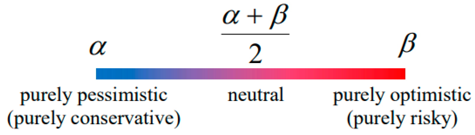
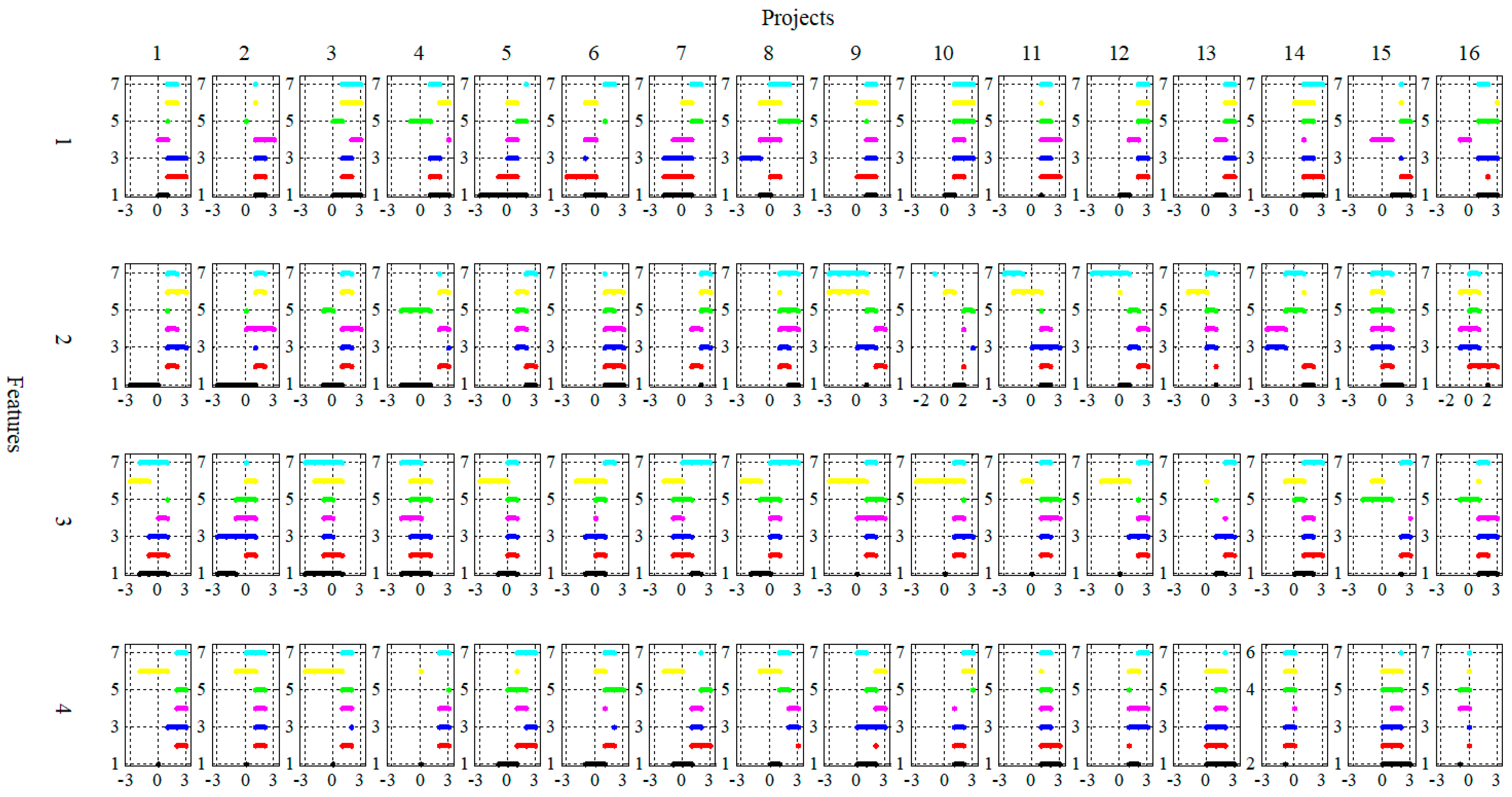
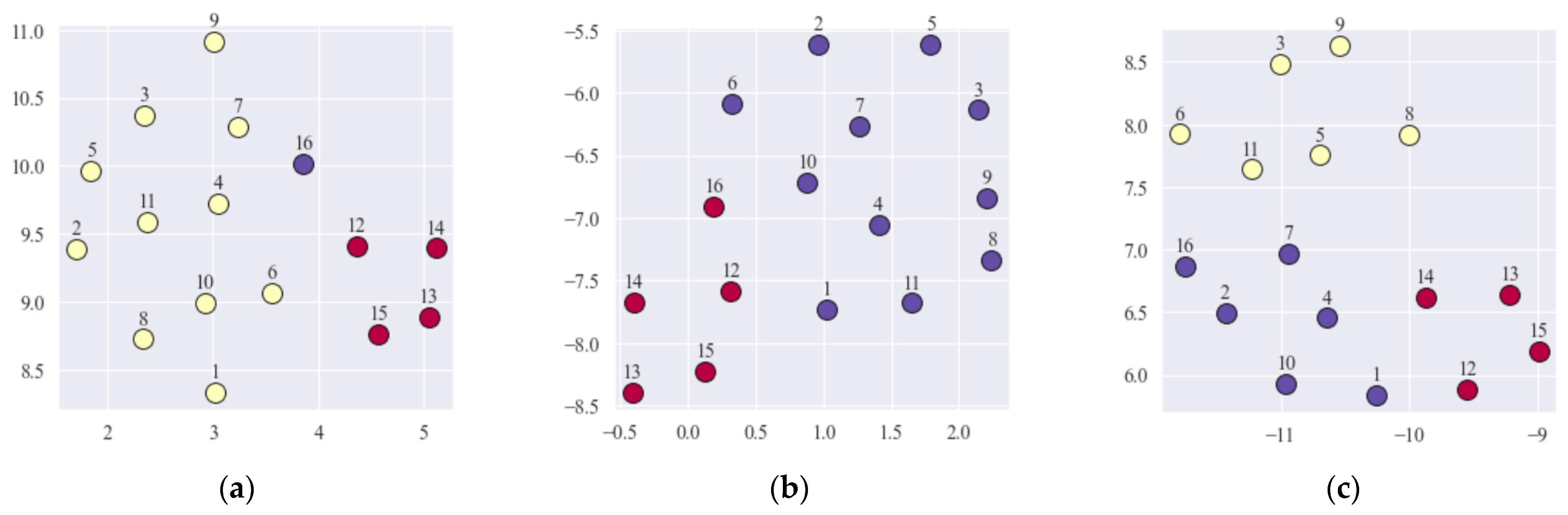
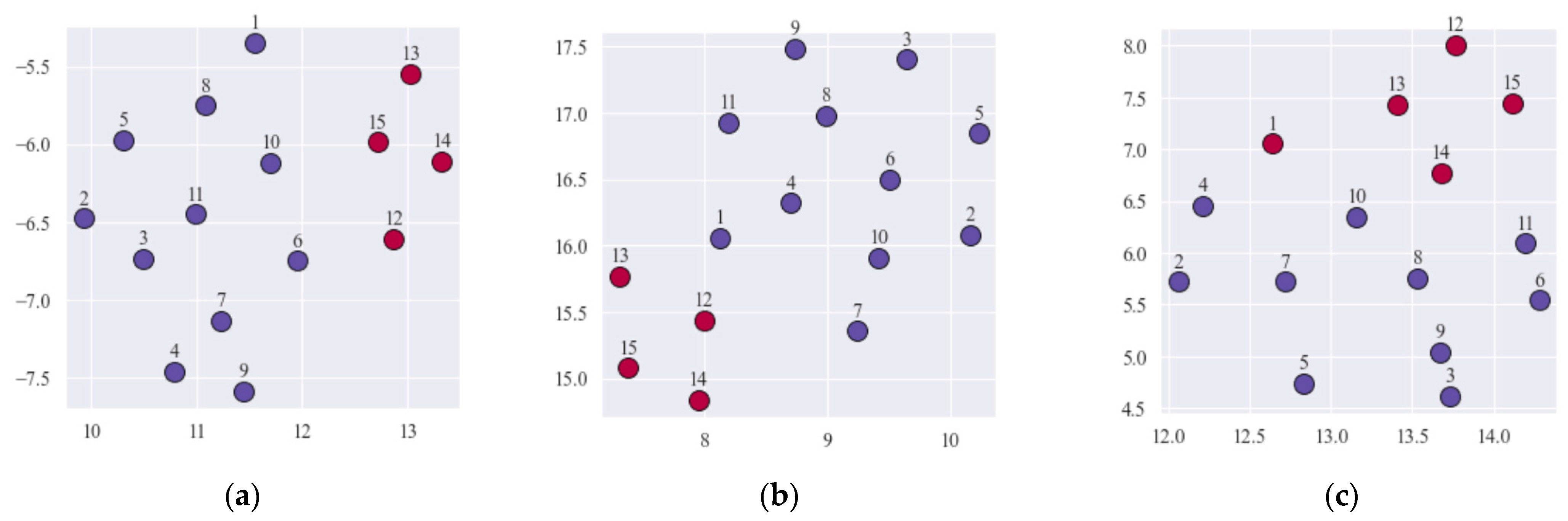
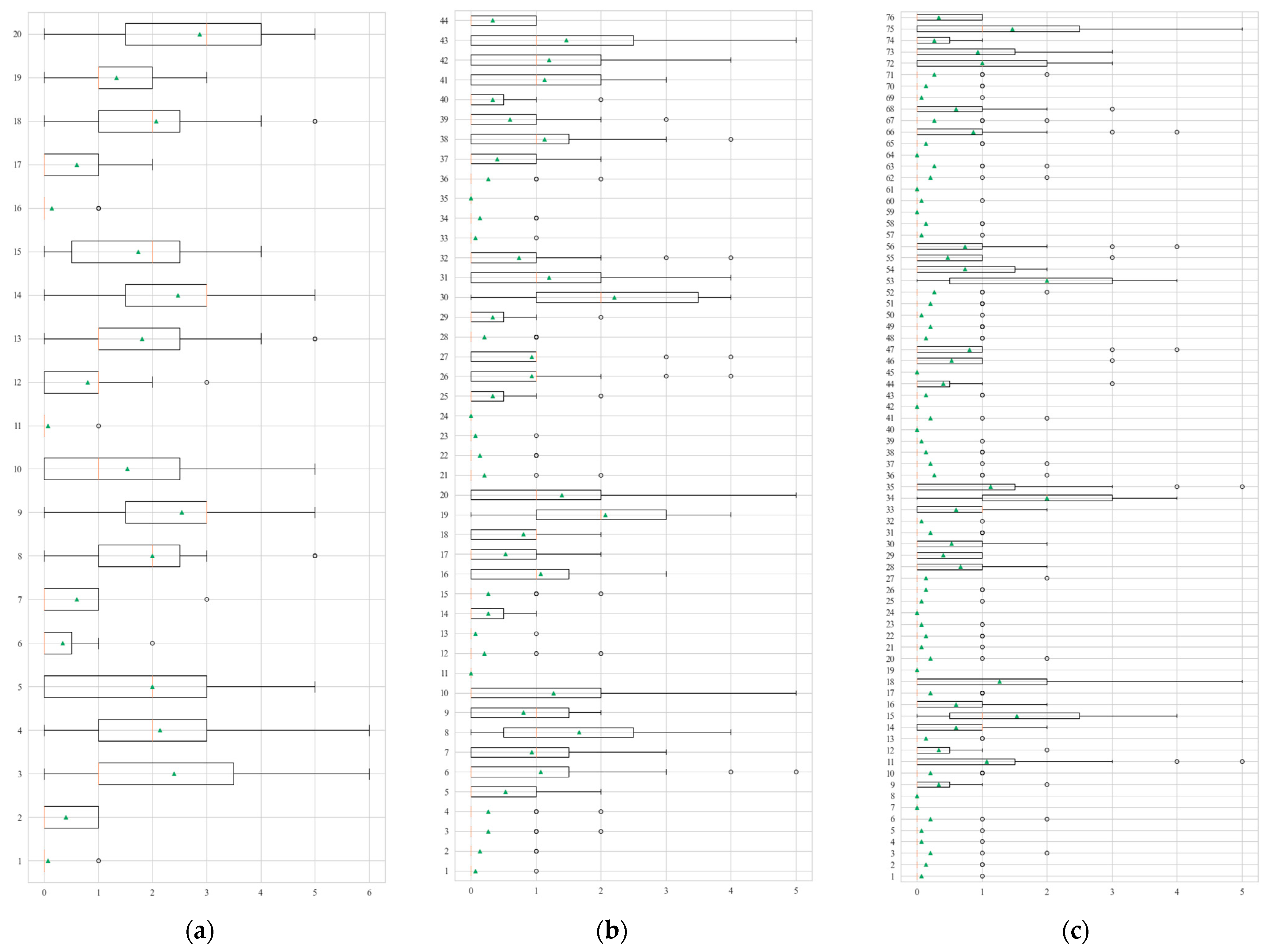
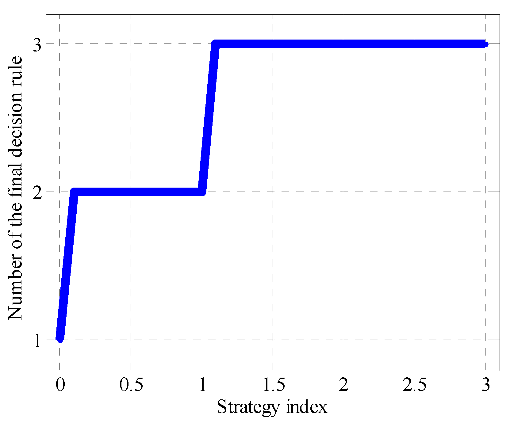
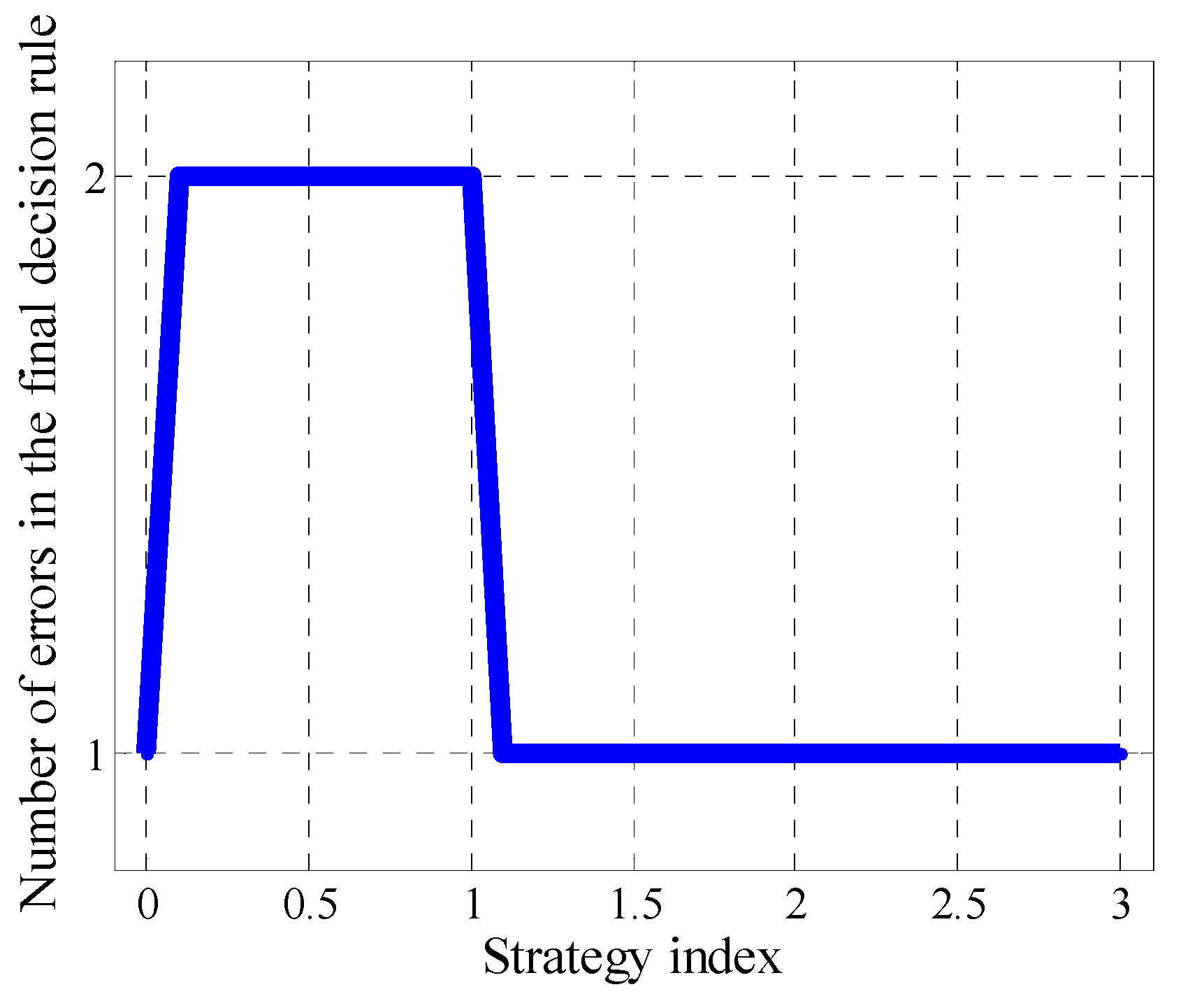
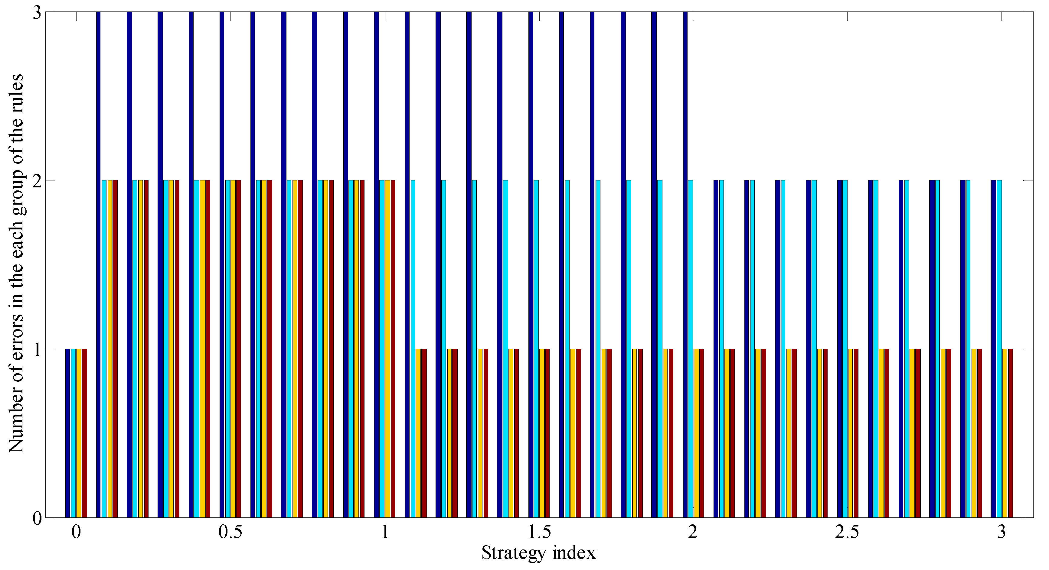
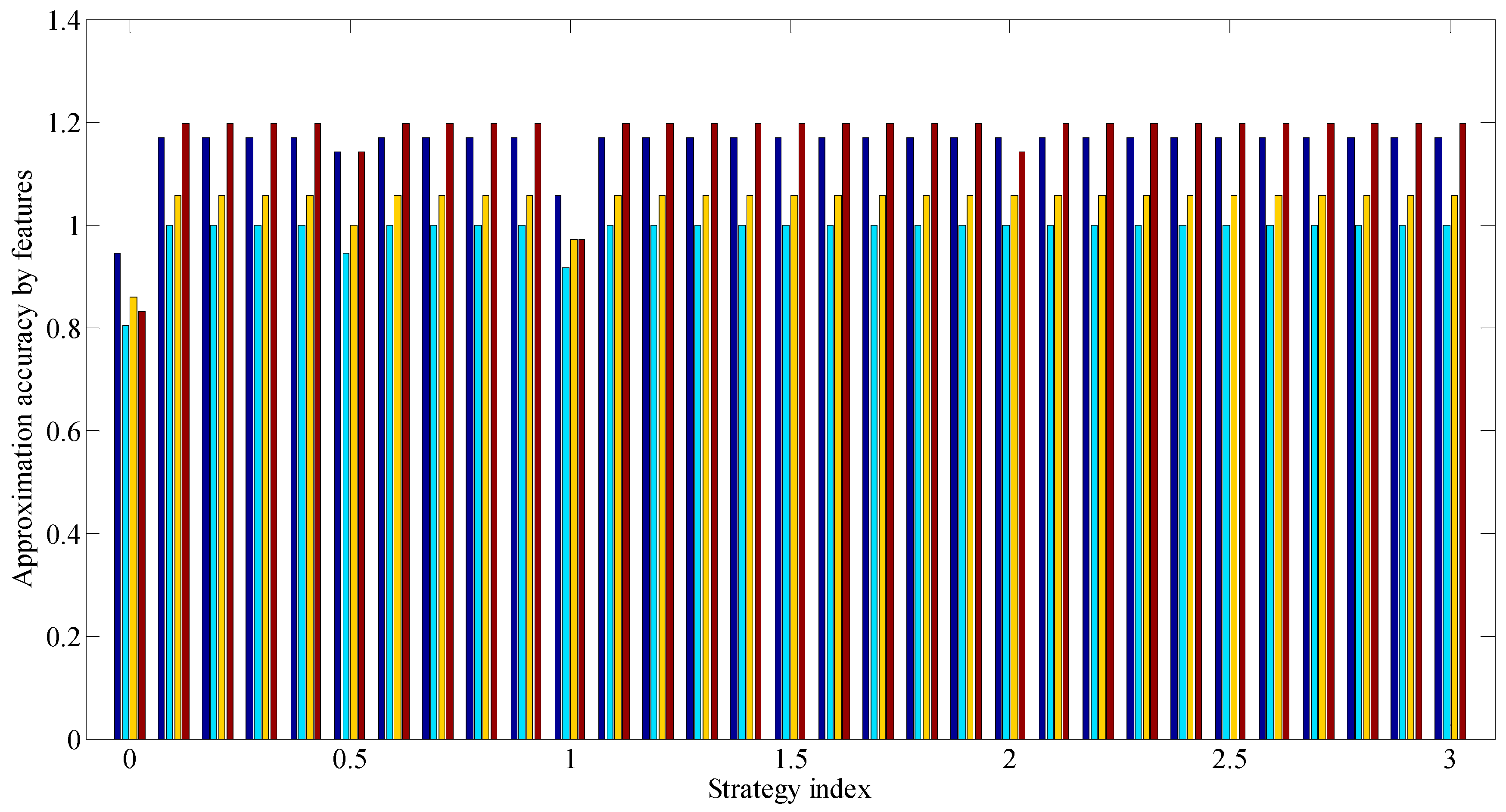
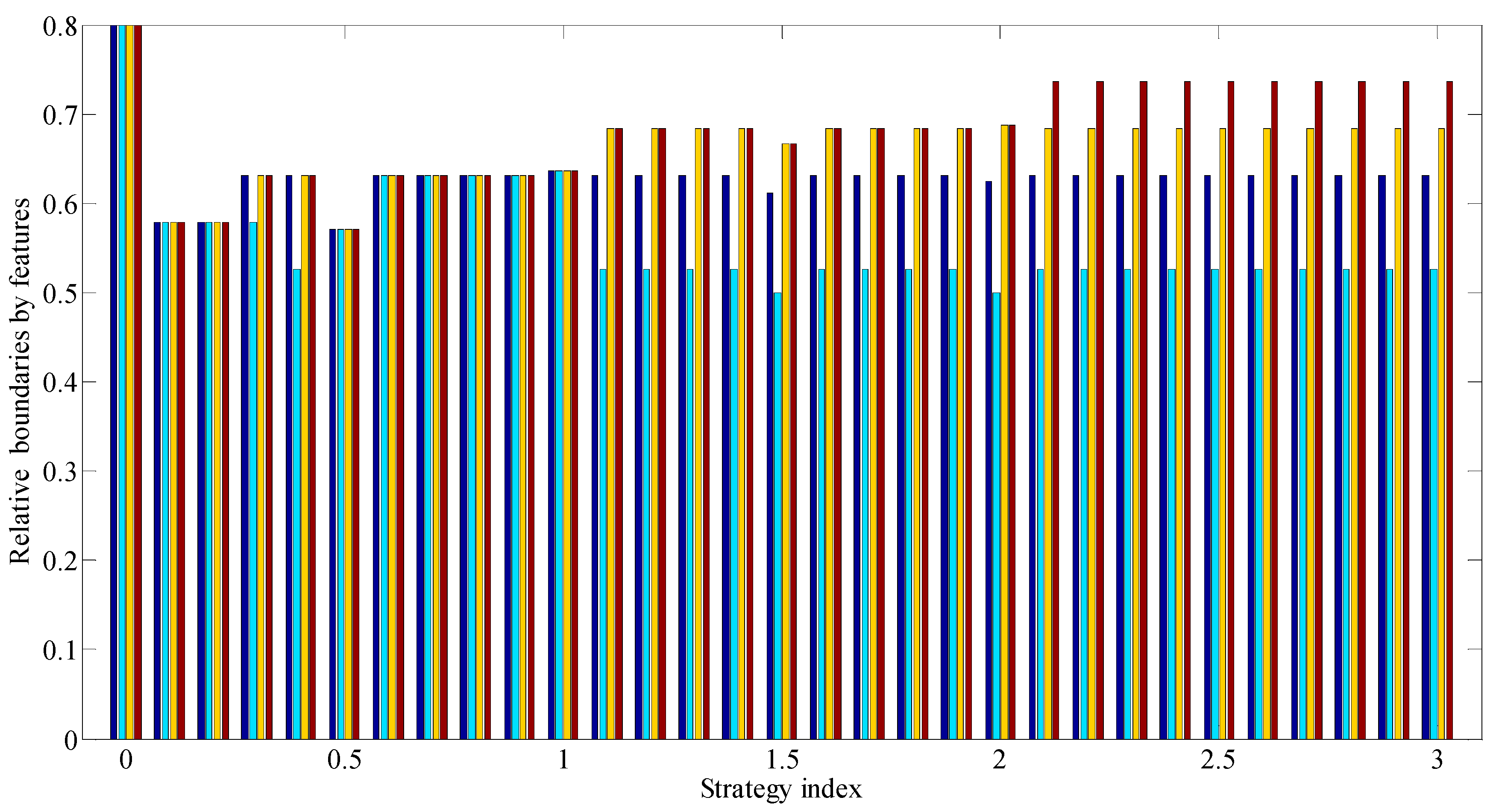
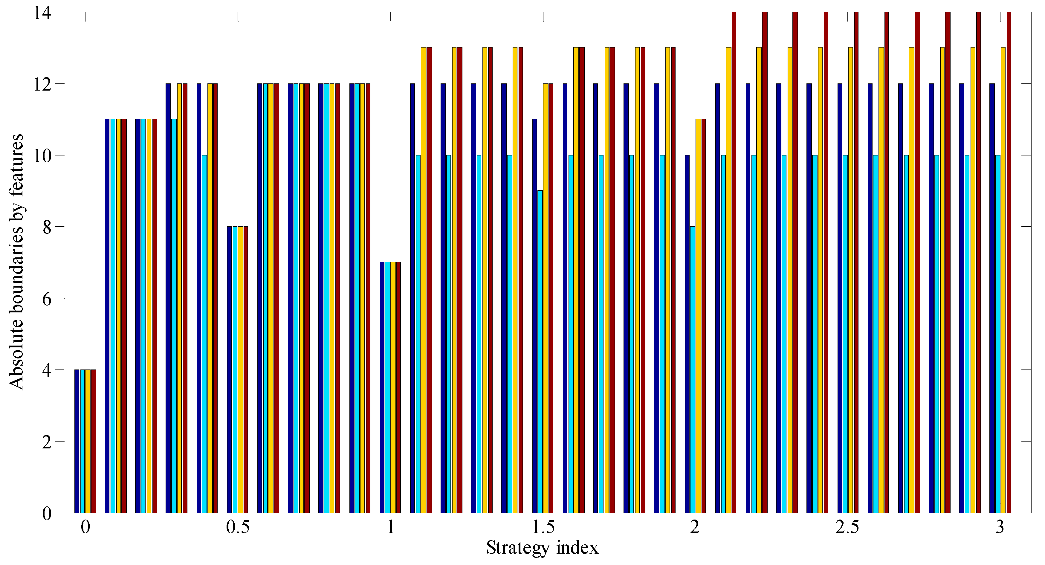
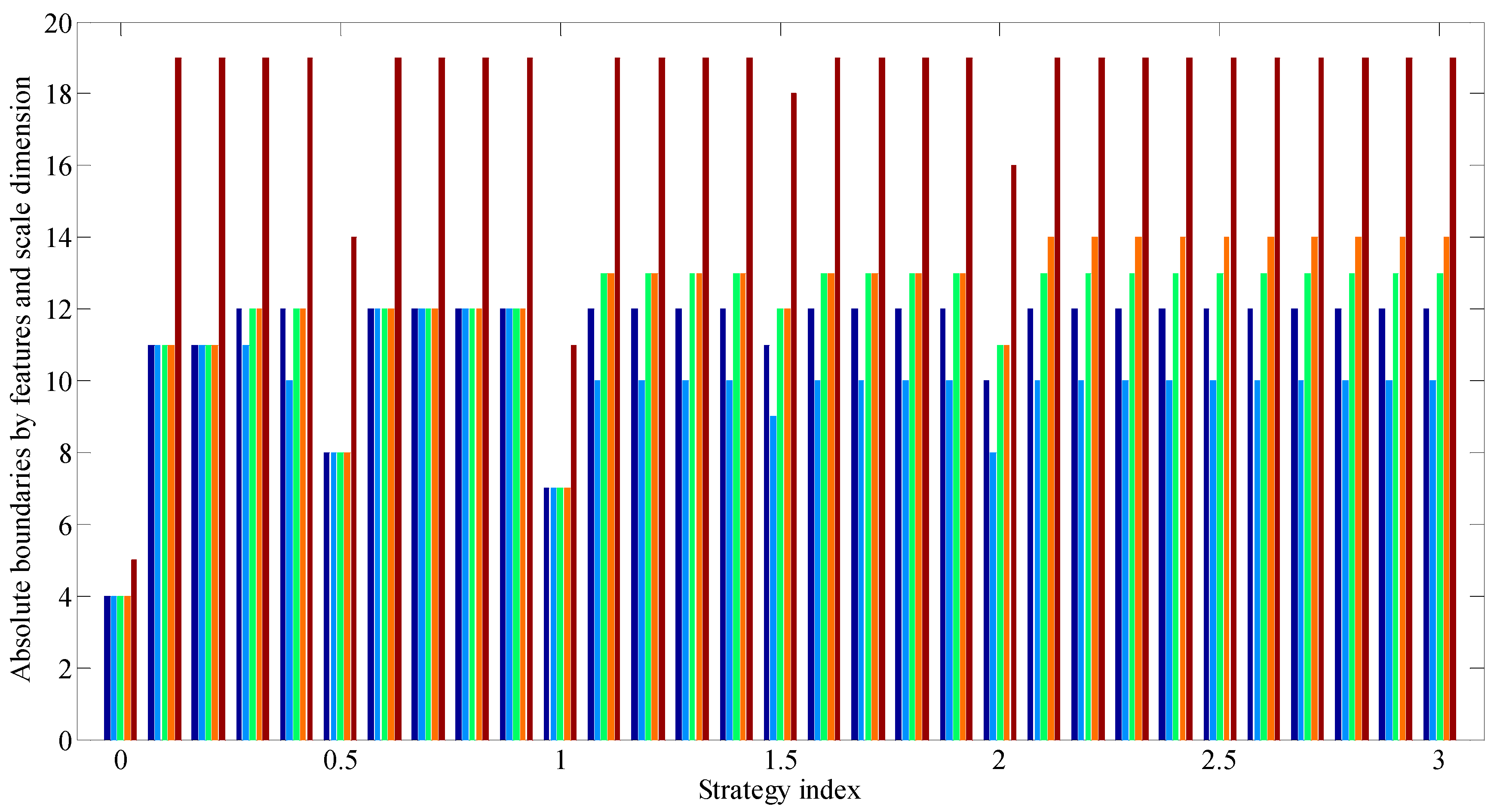
Table 1.
Examples of features scales for purely conservative, neutral and purely risky assessment strategies.
Table 1.
Examples of features scales for purely conservative, neutral and purely risky assessment strategies.
| Strategy | Number of Gradations by Feature | Scores on the Scale (Gradation) in Ascending Order |
|---|---|---|
| Purely conservative | 19 | −2.50; −2.25; −2.00; −1.75; −1.50; −1.25; −1.00; −0.75; −0.50; 0.00; 0.25; 0.50; 0.75; 1.00; 1.25; 1.50; 2.00; 2.25; 3.00 |
| Neutral | 11 | −2.00; −1.50; −1.00; −0.50; 0.00; 0.50; 1.00; 1.50; 2.00; 2.50; 3.00 |
| Purely risky | 5 | −1.00; 0.00; 1.00; 2.00; 3.00 |
Table 2.
Division of competitive projects into classes ‘Accept the CP for implementation’ and ‘Reject the project’.
Table 2.
Division of competitive projects into classes ‘Accept the CP for implementation’ and ‘Reject the project’.
| Features Assessments | Classes | |||||||||||||||||||||
|---|---|---|---|---|---|---|---|---|---|---|---|---|---|---|---|---|---|---|---|---|---|---|
| CP | ||||||||||||||||||||||
| First class | ||||||||||||||||||||||
| 1 | 0 | 0 | 3 | 2 | 2 | 0 | 1 | 2 | 3 | 1 | 0 | 0 | 1 | 2 | 4 | 0 | 0 | 1 | 3 | 3 | 1 | 6 |
| 2 | 0 | 0 | 1 | 6 | 0 | 0 | 0 | 1 | 2 | 4 | 0 | 0 | 2 | 3 | 2 | 0 | 0 | 1 | 1 | 5 | 0 | 7 |
| 3 | 0 | 0 | 0 | 2 | 5 | 0 | 0 | 1 | 3 | 3 | 0 | 0 | 1 | 3 | 3 | 0 | 1 | 0 | 2 | 4 | 1 | 6 |
| 4 | 0 | 1 | 1 | 3 | 2 | 0 | 1 | 2 | 3 | 1 | 0 | 1 | 0 | 4 | 1 | 0 | 0 | 2 | 1 | 4 | 2 | 5 |
| 5 | 0 | 0 | 0 | 4 | 3 | 0 | 0 | 1 | 1 | 5 | 0 | 0 | 0 | 3 | 4 | 0 | 0 | 1 | 2 | 4 | 0 | 7 |
| 6 | 0 | 0 | 3 | 2 | 2 | 1 | 0 | 1 | 3 | 2 | 1 | 0 | 2 | 3 | 1 | 0 | 1 | 2 | 2 | 2 | 2 | 5 |
| 7 | 0 | 1 | 1 | 3 | 2 | 0 | 1 | 0 | 5 | 1 | 0 | 2 | 0 | 3 | 2 | 0 | 1 | 1 | 1 | 4 | 1 | 6 |
| 8 | 0 | 1 | 1 | 2 | 3 | 0 | 0 | 2 | 3 | 2 | 0 | 1 | 1 | 0 | 4 | 0 | 0 | 2 | 2 | 3 | 2 | 5 |
| 9 | 0 | 1 | 1 | 0 | 5 | 0 | 1 | 1 | 5 | 0 | 0 | 1 | 1 | 5 | 0 | 0 | 2 | 0 | 0 | 5 | 1 | 6 |
| 10 | 0 | 0 | 2 | 2 | 3 | 0 | 0 | 3 | 3 | 1 | 0 | 1 | 1 | 3 | 2 | 0 | 0 | 2 | 2 | 3 | 2 | 5 |
| 11 | 0 | 0 | 1 | 3 | 3 | 0 | 0 | 1 | 3 | 3 | 0 | 0 | 1 | 4 | 2 | 0 | 0 | 2 | 2 | 3 | 0 | 7 |
| Second class | ||||||||||||||||||||||
| 12 | 0 | 0 | 4 | 3 | 0 | 1 | 3 | 2 | 1 | 0 | 0 | 0 | 5 | 2 | 0 | 1 | 1 | 3 | 1 | 1 | 5 | 2 |
| 13 | 0 | 1 | 6 | 0 | 0 | 2 | 0 | 3 | 2 | 0 | 0 | 1 | 5 | 1 | 0 | 0 | 0 | 5 | 1 | 1 | 5 | 2 |
| 14 | 1 | 0 | 6 | 0 | 0 | 1 | 1 | 5 | 0 | 0 | 0 | 3 | 4 | 0 | 0 | 0 | 2 | 5 | 0 | 0 | 7 | 0 |
| 15 | 0 | 1 | 6 | 0 | 0 | 0 | 1 | 5 | 1 | 0 | 0 | 2 | 3 | 1 | 1 | 1 | 1 | 4 | 0 | 1 | 6 | 1 |
| Classes | Sums by features and solutions | |||||||||||||||||||||
| 0 | 4 | 14 | 29 | 30 | 1 | 4 | 15 | 34 | 23 | 1 | 6 | 11 | 34 | 25 | 0 | 5 | 14 | 18 | 40 | 12 | 65 | |
| 1 | 2 | 22 | 3 | 0 | 4 | 5 | 15 | 4 | 0 | 0 | 6 | 17 | 4 | 1 | 2 | 4 | 17 | 2 | 3 | 23 | 5 | |
| 67 | 57 | 61 | 59 | 71 | ||||||||||||||||||
| 0.944 | 0.803 | 0.859 | 0.831 | |||||||||||||||||||
| Noise | ||||||||||||||||||||||
| 16 | 0 | 0 | 0 | 6 | 1 | 1 | 6 | 0 | 0 | 0 | 0 | 0 | 0 | 6 | 1 | 1 | 6 | 0 | 0 | 0 | 4 | 3 |
Table 3.
GDRCs allowing to classify CP as ‘Accept CP for implementation’, when using the purely risky assessment strategy.
Table 3.
GDRCs allowing to classify CP as ‘Accept CP for implementation’, when using the purely risky assessment strategy.
| Rule | P1 | P3 | P4 | P2 | Approximation Indicator |
|---|---|---|---|---|---|
| 1 | 2 or 3 | – | – | – | 0.944 |
| 2 | 2 or 3 | 2 or 3 | – | – | 0.859 |
| 3 | 2 or 3 | 2 or 3 | 2 or 3 | – | 0.831 |
| 4 | 2 or 3 | 2 or 3 | 2 or 3 | 2 or 3 | 0.803 |
Table 4.
CPs ranks in the ordering list.
| CP | Assessment Strategy (δ) | ||||
|---|---|---|---|---|---|
| 0 (Purely Risky Strategy) | 0.1–0.2 | 0.3–0.9 | 1 (Neutral Strategy) | 1.1–3 (Purely Conservative Strategy) | |
| 1 | 6 | 6 | 6 | 6 | 6 |
| 2 | 3 | 4 | 4 | 4 | 4 |
| 3 | 2 | 2 | 2 | 2 | 2 |
| 4 | 10 | 10 | 10 | 10 | 10 |
| 5 | 1 | 1 | 1 | 1 | 1 |
| 6 | 11 | 11 | 11 | 11 | 11 |
| 7 | 8 | 9 | 9 | 9 | 9 |
| 8 | 5 | 5 | 5 | 5 | 5 |
| 9 | 9 | 8 | 8 | 7 | 7 |
| 10 | 7 | 7 | 7 | 8 | 8 |
| 11 | 4 | 3 | 3 | 3 | 3 |
| 12 | 12 | 12 | 13 | 13 | 12 |
| 13 | - | 13 | 12 | 12 | - |
Publisher’s Note: MDPI stays neutral with regard to jurisdictional claims in published maps and institutional affiliations. |
© 2021 by the authors. Licensee MDPI, Basel, Switzerland. This article is an open access article distributed under the terms and conditions of the Creative Commons Attribution (CC BY) license (https://creativecommons.org/licenses/by/4.0/).
Share and Cite
MDPI and ACS Style
Demidova, L.A.; Sokolova, J.S. Analysis of Data Presented by Multisets Using a Linguistic Approach. Algorithms 2021, 14, 135. https://0-doi-org.brum.beds.ac.uk/10.3390/a14050135
AMA Style
Demidova LA, Sokolova JS. Analysis of Data Presented by Multisets Using a Linguistic Approach. Algorithms. 2021; 14(5):135. https://0-doi-org.brum.beds.ac.uk/10.3390/a14050135
Chicago/Turabian StyleDemidova, Liliya A., and Julia S. Sokolova. 2021. "Analysis of Data Presented by Multisets Using a Linguistic Approach" Algorithms 14, no. 5: 135. https://0-doi-org.brum.beds.ac.uk/10.3390/a14050135
Note that from the first issue of 2016, this journal uses article numbers instead of page numbers. See further details here.