
No-Wait Job Shop Scheduling Using a Population-Based Iterated Greedy Algorithm

Key Laboratory of Cyber-Physical System and Intelligent Control in Universities of Shandong, School of Information and Electrical Engineering, Ludong University, Yantai 264025, China
*
Author to whom correspondence should be addressed.
Algorithms 2021, 14(5), 145; https://0-doi-org.brum.beds.ac.uk/10.3390/a14050145
Submission received: 2 April 2021
/
Revised: 24 April 2021
/
Accepted: 28 April 2021
/
Published: 30 April 2021
(This article belongs to the Section Combinatorial Optimization, Graph, and Network Algorithms)
Abstract
:When no-wait constraint holds in job shops, a job has to be processed with no waiting time from the first to the last operation, and the start time of a job is greatly restricted. Using key elements of the iterated greedy algorithm, this paper proposes a population-based iterated greedy (PBIG) algorithm for finding high-quality schedules in no-wait job shops. Firstly, the Nawaz–Enscore–Ham (NEH) heuristic used for flow shop is extended in no-wait job shops, and an initialization scheme based on the NEH heuristic is developed to generate start solutions with a certain quality and diversity. Secondly, the iterated greedy procedure is introduced based on the destruction and construction perturbator and the insert-based local search. Furthermore, a population-based co-evolutionary scheme is presented by imposing the iterated greedy procedure in parallel and hybridizing both the left timetabling and inverse left timetabling methods. Computational results based on well-known benchmark instances show that the proposed algorithm outperforms two existing metaheuristics by a significant margin.
1. Introduction
No-wait constraints widely exist in the steel-making industry (Pinedo [1]; Tang et al. [2]), concrete manufacturing (Grabowski and Pempera [3]), chemical and pharmaceutical industries (Rajendran [4]), food industries (Hall and Sriskandarajah [5]), and so on. The job shop problem with no-wait constraints is called the no-wait job shop scheduling problem (NWJSP) and it differs from traditional job shop problem (JSP) a lot because of the no-wait constraints. NWJSP has gained the increasing attention of researchers over decades. With regard to its complexity, NWJSP is NP (non-deterministic polynomial time)-hard in the strong sense (Lenstra et al. [6]). Sahni and Cho [7] proved that it is strongly NP-hard even for two machine cases. Mascis and Pacciarelli [8] formulated it as an alternative graph and presented several heuristics and a branch and bound method. Broek [9] formulated the problem as a mixed integer program (MIP) and presented a branch and bound method. Recently, Bürgy and Gröflin [10] provided a compact formulation of the problem and proposed an effective approach based on optimal job insertion.
Due to the NP-hardness of NWJSP, the focus has been mostly on metaheuristic approaches for the problem. The pioneer work conducted by Macchiaroli et al. [11] decomposed the problem into two sub-problems and gave out a two-phase tabu search algorithm that is superior to dispatching rules. Schuster and Framinan [12] presented a variable neighborhood search (VNS) algorithm and a hybrid algorithm of simulated annealing and generic algorithm (GASA). Later, Schuster [13] developed a fast tabu search (TS) method, and Framinan and Schuster [14] proposed a complete local search with memory (CLM). Zhu et al. [15] investigated the timetabling methods and developed a complete local search with limited memory (CLLM), which was shown to be comparable to the VNS, GASA and CLM. Zhu and Li [16] also proposed an efficient shift penalty-based timetabling method and further put forward a modified complete local search with memory (MCLM). Mokhtari [17] presented a neuro-evolutionary variable neighborhood search which is based on the combination of an enhanced variable neighborhood search and an artificial neural network. The proposed algorithm was shown to be applicable and effective for the problem. Very recently, Aitzai et al. [18] proposed a branch and bound method and a particle swarm optimization algorithm for the problem. They compared the proposed algorithms with several heuristics but bypassed the other metaheuristics. Li et al. [19] improved the CLLM and developed a complete local search with memory and variable neighborhood structure (CLMMV) algorithm. The CLMMV was shown to have similar effectiveness to and better efficiency than the CLLM. More recently, Sundar et al. [20] proposed a hybrid artificial bee colony (HABC) algorithm and stated that the HABC outperforms the MCLM, as well as the CLLM.
According to the decomposition scheme in Macchiaroli et al. [11], the NWJSP can be decomposed into a timetabling problem and sequencing problem. The sequencing problem is to find a processing sequence of an optimal schedule, whereas the timetabling problem is to determine a feasible starting time for each job in the processing sequence. Using this decomposition scheme, the NWJSP can be solved in a similar way as the flow shop scheduling problem. As an effective and efficient procedure, the iterated greedy (IG) algorithm originally presented by Ruiz and Stutzle [21] has been applied in various scheduling environments, such as identical parallel machine scheduling [22], the distributed flow shop scheduling problem [23], and the blocking flow shop scheduling problem [24]. The IG has shown its unique potentials and advantages of fast convergence, good effectiveness, and easy implementation. In this study, we try to introduce and adapt the IG for the NWJSP. In order to enhance the diversity of the algorithm, we introduce a co-evolutionary scheme, and present a population-based IG algorithm.
The rest of the paper is organized as follows. In Section 2, the NWJSP is formulated into two sub-problems: the timetabling problem and the sequencing problem. Section 3 presents the iterated greedy algorithm and the competitive co-evolutionary scheme. Section 4 analyzes the computational results. Finally, concluding remarks are given in Section 5.
2. No-Wait Job Shop Scheduling Problem (NWJSP) with Makespan Minimization
2.1. Problem Statement
The NWJSP involves a set of machines and a set of jobs which have to be processed on the machines. Each job has its own processing route, namely its own sequence of operations. Each operation is associated with a processing time and a processing machine. The no-wait constraint holds for each job, which means no waiting time is allowed between two consecutive operations of the same job. Besides, we have the following assumptions: (1) all the jobs and machines are available at time zero; (2) at any time, a machine can process at most one job, and a job can be processed on at most one machine; (3) preemption is not allowed; (4) the set-up, release, and transfer time is incorporated in the processing time; (5) no job is allowed to reenter previous machines.
The objective is to find a feasible schedule that minimizes the maximum completion time of all jobs, namely the makespan.
2.2. Problem Formulation
For two jobs Ji and Jj, let u and v be their two operations that are processed on the same machine (). According to the no-wait constraint, the completion time of operation u and v is and , respectively. Operation u is either anterior or posterior to operation v. Therefore, we have , which is equivalent to:
Using the above condition (1), the problem with the makespan criterion can be described as follows:
tn+1 is the start time of a dummy job, representing the makespan. Constraint (3) means that each job starts after time zero. Constraint (4) guarantees that the no-wait requirement is satisfied for any two jobs. Note that the number of constraint (4) is reduced by using i < j instead of .
For the above operation pair , let Mk denote the same machine of operations u and v, then , , , mean the same as , , , , respectively. Condition (1) can be rewritten as:
For two jobs Ji and Jj, if their start time difference satisfies condition (5), then these two jobs do not conflict on machine Mk.
Obviously, the start times ti and tj are feasible if and only if jobs Ji and Jj do not conflict on all machines, which means that tj − ti satisfies condition (5) for all machines Mk (k = 1, 2, …, m). Therefore, constraint (4) can be described as , where Fij is an interval set with the feasible values of , obtained by:
With the above notations, the NWJSP with the makespan criterion is further formulated as follows:
Li and all Fij can be computed in advance. According to Equation (6), all Fij can be computed in time O(n2mlogm). Fij is an interval set with at most m + 1 intervals.
The existing effective approaches for the problem usually decompose it into the sequencing and timetabling sub-problems. The purpose of the sequencing sub-problem is to find a job sequence, denoted here as , that generates a schedule minimizing the makespan. Clearly, the search space of the sequencing sub-problem has solutions. The purpose of the timetabling sub-problem is to find a timetable, , with a minimum based on a given job sequence .
2.3. Timetabling Methods
There are several timetabling methods to determine a feasible schedule from a provided job permutation. The combinations of different timetabling methods and different sequencing algorithms are extensively studied by Samarghandi et al. [25]. They found that complicated methods are not necessarily superior to simple methods, and some simpler methods prove to be more effective. Deng et al. [26] investigated several timetabling methods for the problem with total flow time criterion and found that the left timetabling and inverse left timetabling methods are more effective when the algorithm for the sequencing problem is run with the same computational efforts. In the left timetabling method, we set t[1] = 0, and compute the minimum t[i] successively for i = 2,…,n, subjected to (1) and (2) does not conflict with for all j < i. The inverse left timetabling method is the same as the left timetabling method except that it is performed on the inverse instance. The inverse left timetabling method is based on the fact that a solution for the inverse instance is also applicable for the original instance (see more in Schuster [13] and Zhu et al. [15]).
As stated above, means the start times of and are feasible. Let , then means the start times of and are feasible and starts not earlier than . All and can be computed in advance with time complexity . Without loss of generality, assume that the permutation is . The left timetabling of π utilizes all the precomputed () and (). First let . Then is computed successively from to . For job , with the already computed (), the steps to compute is designed as follows.
Step 1: set as the minimum value that satisfies the first interval of .
Step 2: check , …, , successively. When checking () or (), if the incumbent does not satisfy any interval of () or (), augment to make it satisfied and then check , …, , successively again. This step is repeated until satisfies all the , …, , .
Since there are at most intervals in or , when the worst case happens, to compute needs time complexity , and to compute all the (j = 1, …, n) needs time complexity , which results in the worst case time complexity for the left timetabling. According to Deng et al. [26], the above procedure is effective for the left timetabling method and inverse left timetabling method.
3. Population-Based Iterated Greedy Algorithm
In this section, we try to introduce and adapt the IG for the NWJSP. We first develop an IG algorithm as a combination of a perturbator and an insertion-based local search. Thereafter, we introduce a co-evolutionary scheme and present a population-based IG (PBIG) algorithm. Most of the algorithms in the existing studies apply one timetabling method, whereas the PBIG in this study uses both the left timetabling and inverse left timetabling methods to enhance the quality of schedule solutions.
3.1. Iterated Greedy Procedure
In the framework of IG for permutation flow shop scheduling problem (PFSP), the incumbent solution is updated by iterating over three phases. Firstly, the destruction and construction (DC) operator is used as a perturbator to generate a candidate solution usually different from the incumbent solution. Then an iterative improvement local search is applied to the candidate solution and a new solution is obtained. Finally, an acceptance criterion decides whether the new solution will replace the incumbent one. In this paper, these phases are applied to NWJSP as follows.
3.1.1. Destruction and Construction
The DC operator consists of two phases: destruction phase and construction phase. In destruction phase, d jobs are randomly selected, removed from the incumbent permutation π. Then in the construction phase, all the deleted jobs are reinserted, one by one, into π to construct a complete permutation. The procedure of the DC is shown in Algorithm 1, where the final πF is the candidate solution found by the DC.
| Algorithm 1. The destruction and construction (DC) operator. |
| 1: choose d unrepeated jobs s1, …, sd randomly, delete them from π, and a sequence with n – d jobs is obtained. 2: for i from 1 to d 3: insert si into the n – d + i positions of πF, evaluate the obtained n – d + i sequences, and replace πF with the best one. 4: endfor. |
3.1.2. Local Search
The local search is performed on the candidate solution found by the DC. In the local search of the IG algorithm by Ruiz and Stutzle [21], a job s is extracted from the permutation π and inserted into the other n − 1 possible positions. Let denote the permutation of the best insert move, namely the permutation resulting in the best makespan among the n − 1 permutations. If is better than π, π is replaced with . The process is then repeated for another job, and it terminates when no improvement occurs for all jobs. Deng et al. [26] improved this local search by avoiding redundant search, and developed insert-based local search (IBLS). Here we introduce the IBLS for the makespan criterion. The procedure of the IBLS is shown in Algorithm 2. The IBLS employs a random permutation at the very beginning to make the local search more stochastic.
| Algorithm 2. Insertion-based local search (IBLS). |
| 1: = a permutation generated randomly 2: i = 0, h = 1 3: while (i < n) 4: let s = 5: find 6: if ( is better than π) 7: 8: i = 1 9: else 10: i = i + 1 11: endif 12: h = (h + 1) % n 13: endwhile |
3.2. Initialization
Since the PBIG is a pullulation-based algorithm, there is a population with p solutions evolving in the algorithm. Each solution is performed with the IG procedure. The Nawaz–Enscore–Ham (NEH) heuristic (Nawaz et al. [27]) has been shown to be one of the most effective heuristics for flow shop problems, and it has been extensively utilized to generate initial solutions for metaheuristics for the flow shop problems. The NEH heuristic firstly sequences the jobs in non-increasing order of the total processing time on all the machines. Then it constructs a partial solution by taking into consideration the first two jobs. Finally, a complete solution is constructed by inserting these jobs one by one into the current partial solution.
To adapt the NEH heuristic for NWJSP, the evaluation of a partial sequence in NWJSP is different from that in PFSP. For a partial sequence, here the timetabling method is applied to construct a partial time table as a partial solution. With this, the NEH heuristic is described as follows.
Step 1: sequence the jobs in non-increasing order of the total processing time on all the machines and obtain a priority job order Let partial sequence and k = 2.
Step 2: insert job to all the possible k positions of σ and obtain k tentative partial sequences. Evaluate these partial sequences by applying the timetabling method, replace σ with the partial sequence that results in the minimum makespan.
Step 3: Let k = k + 1. If k ≤ n, go to step 2; otherwise σ is the final permutation.
To employ the NEH heuristic to generate a random solution with good quality, we use a random job permutation as job order in the first step, and develop a variant of the NEH heuristic, called NEH_RAN. It should be noted that both the left timetabling and inverse left timetabling methods can be used in the above NEH heuristic and its variants. In other words, the heuristic can be applied with the left timetabling for the original instance to obtain a solution, and it can also be applied with the inverse timetabling for the inverse instance to obtain another solution.
To take advantage of both the left timetabling and inverse left timetabling methods, both methods are applied in the p IG procedures. A bool vector md = (md(1),…, md(p)) is designed to indicate the timetabling method for the p IG procedures. md(k) = true means that the k-th IG procedure is performed with the left timetabling, otherwise it is performed with the inverse left timetabling. md is initialized in a form of (true, false, true, false, …). Then, the p initial solutions of the p IG procedures are initialized as follows.
The first is initialized by the NEH heuristic using the left timetabling, and the second is initialized by the NEH heuristic using the inverse left timetabling. The remaining p − 2 initial solutions are initialized by the NEH_RAN using the inverse left timetabling (if the md(k) value is true) or using the inverse left timetabling (if the md(k) value is false). Such an initialization strategy not only takes advantage of both the timetabling methods, but also constructs the initial start solutions with both quality and diversity.
3.3. Competitive Co-Evolutionary Scheme
Three best solutions, πL, πI and πG, are stored together in the algorithm. πL is the best solution found by all IG procedures with respect to left timetabling method, while πI is the best solution found by all IG procedures with respect to inverse left timetabling method. πG is the better of πL and πI, namely the global best solution found so far. πL, πI and πG are initialized based on the p initial solutions.
After the p initial solutions are generated, the p IG procedures go into iteration simultaneously. Each IG procedure evolves according to its own timetabling method, either left timetabling or inverse left timetabling. It can be easily inferred that as the evolution proceeds, the incumbent solutions found by the IG algorithms are probably not the same, which means some of the incumbent solutions may be relatively better than others. Therefore, a reasonable assumption is that when an iteration is accomplished, some advantage should be taken of the relatively better solutions. Based on this assumption, the tournament selection is introduced as a competitive strategy. In the tournament selection, firstly, three solutions are randomly selected, and then the worst one is replaced with a perturbation solution which is generated by performing the DC on πL or πI with parameter D. Let (k = 1, …, p) denote the incumbent solution of the k-th IG procedure, and let mdbest denote the bool value indicating the timetabling method for πG. The competitive strategy is illustrated in Algorithm 3, where rand is a real number randomly generated in [1]. Note that mdbest = true means that πG is the same as πL, otherwise it is the same as πI. The perturbation solution is generated based on the global solution πG with probability pb. Considering that the global solution πG should be given more chances than the other best solution, the suggested value of pb are between 0.5 and 1.0.
| Algorithm 3. Competitive Strategy. |
| 1: randomly select three solutions from all and find the worst one. 2: if (rand < pb) 3: πC := πG 4: md(k*) := mdbest 5: else if (mdbest) 6: πC := πL 7: md(k*) := true 8: else 9: πC := πI 10: md(k*) := false 11: endif 12: endif 13: perform DC on with parameter D and obtain a perturbation solution 14: := |
3.4. Procedure of the Population-Based Iterated Greedy (PBIG) Algorithm
Since the details of all components of the PBIG have been given, the whole computational procedure is outlined in Algorithm 4. Such an algorithm is expected to solve the NWJSP with the makespan criterion effectively and efficiently. It should be noted that although the PBIG in this study has an analogous framework with the population-based iterated greedy (denoted PBIG_D here) algorithm in [26], they are different in several facets. Firstly, the PBIG in this study is applied to the makespan criterion, whereas the PBIG_D is designed for the total flow time criterion. Secondly, different optimization criteria cause different characteristics for the NWJSP, including the distribution features of the solutions and the effects of timetabling methods. Therefore, the PBIG uses both the left timetabling and inverse left timetabling methods, whereas the PBIG_D only employs the left timetabling method. Lastly, the PBIG contains a newly-designed competitive scheme, where the perturbation solution is generated based on a solution with either of the two timetabling methods, whereas in the competitive mechanism of the PBIG_D, the shaking solution is simply generated from the best solution found so far.
| Algorithm 4. Procedure of the PBIG. |
| 1: set parameters d, p, D, pb. 2: initialize πk (k = 1, …, p), πL, πI, πG, md, mdbest, Temp. 3: while (not termination) 4: for (each πk) //perform each IG procedure 5: perform the DC operator on πk and then the IBLS, and obtain a new solution . If is better than πk, then let πk := and update πL, πI, πG, mdbest if possible. 6: endfor 7: perform competitive strategy. 8: endwhile |
4. Computational Results and Comparisons
Computational experiments are performed on the following well-known benchmark instances: ft06, ft10, ft20 (Fisher and Thompson [28]), orb01-10 (Applegate and Cook [29]), abz5-9 (Adams et al. [30]), la01-40 (Lawrence [31]), and swv01-20 (Storer et al. [32]). The algorithm is programmed in C++ language and the running environment is a PC with Intel Core(TM) i5-6200 2.3 GHz processor. The acceleration method for insert neighborhood in [33] is used in order to save computational efforts. The following relative percentage deviation (RPD) is calculated to indicate the effectiveness:
where CALG is the solution obtained by the tested algorithm, and CREF is the reference solution. In this study, we use the same reference solution as in [16,20].
4.1. Calibration of the PBIG Algorithm
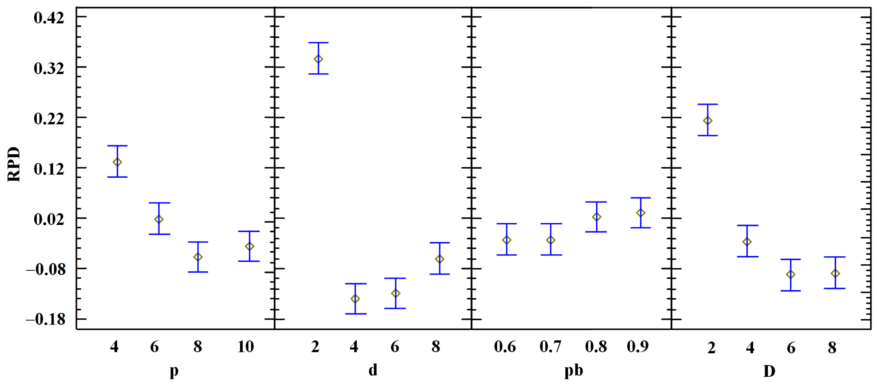
There are four parameters in total to calibrate for the PBIG, namely p, d, pb, and D. A larger Design of Experiments (DOE) [34] is carried out based on the following factor: (1) parameter p tested at four levels: 4, 6, 8, 10; (2) parameter d tested at four levels: 2, 4, 6, 8; (3) parameter pb tested at four levels: 0.6, 0.7, 0.8, 0.9; (4) parameter D tested at four levels: 2, 4, 6, 8. We select the following seven instances with different sizes from each other: la06, la11, la21, la26, la31, la36, and swv01. Each instance is solved by the algorithm for each combination of the factors with five independent replications. The average RPD (ARPD) obtained by the algorithm is calculated as a response variable. The stopping criterion is the elapsed CPU time not less than 6 mn2 milliseconds (ms). The multi-factor Analysis of Variance (ANOVA) technique is used to analyze the computational results. The ANOVA results are shown in Table 2. It can be seen from Table 2 that the parameters p, d, and D are statistically significant, whereas the parameter pb is not. The means plots of these factors, together with least significant difference (LSD) 95% confidence intervals, are illustrated in Fig. 1. Recall that if the LSD intervals for two means are not overlapping, then the difference between the two means is statistically significant.
Figure 1 suggests that for the values of parameter p, 8 is statistically better than 4 and 6, although its difference from 10 is not significant. For the values of parameter d, 4 is statistically better than 2 and 8. The values 6 and 8 are relatively better than 2 and 4 for the parameter D, while no statistical significance is found for the parameter pb. Finally, the parameters of the algorithm are set as p = 8, d = 4, pb = 0.7, and D = 6.
4.2. Comparisons with Other Metaheuristics
Among the metaheuristics developed for the NWJSP in the literature, the MCLM [16] and the HABC [18] algorithms are two state-of-the-art approaches. Therefore, these two algorithms are used to compare with the proposed PBIG in this subsection. We bypassed the other algorithms either because it provided a low-level performance or because it was hard to compare with the PBIG due to different performance indexes. Like the MCLM and HABC algorithms, the PBIG is applied to 22 small instances and 40 large instances with 20 replications. It should be noted that the MCLM was implemented in Java on a Pentium 4 processor and its average central processing unit (CPU) time was 6.55 s for the small instances and 654.48 s for the large instances, while the HABC was implemented in C on an identical processor and its average CPU time was 4.63 and 570.40 s for the small and large instances, respectively. Both the MCLM and the HABC adopted a stopping criterion determined by the current results found by the algorithm, and thus the computational time of the algorithm was not controllable. Such kind of stopping criterion makes it difficult to compare the algorithms in a fair way. Take instance Swv09 as an example, the average CPU time of the MCLM was 448 s whereas that of the HABC was 1531.08 s, and it was difficult to determine which algorithm was better although the RPD results of the MCLM were worse than those of the HABC. For this reason, the stopping criterion of the PBIG was set as the elapsed CPU time not less than 3 mn2 ms for the small instances and 60 mn2 ms for the large instances to facilitate the comparisons under the same criterion by future researchers. Using this stopping criterion, the PBIG required less average CPU time than the MCLM and HABC. We adopt the original results from [16,18] and do not reimplement the MCLM and HABC. The computational results are given in Table 3 and Table 4 for the small and large instances, respectively. In Table 3 and Table 4, TA denotes the average CPU time (in seconds) of 20 runs. Best denotes the best makespan value among 20 runs for the corresponding algorithm. RPDB denotes the RPD value of the Best. ARPD denotes the average RPD value over 20 runs. Best results among the three algorithms are shown in bold for Best, RPDB, and ARPD. NA denotes that the value was not provided in the original results. The column noted as BKS shows the reference solution used in the RPD. Note that the BKS values in Table 3 are also optimal solutions of the small instances.
Table 3 shows that the PBIG can optimally solve all the small instances except Orb05. Further, for all the instances except Orb05 and La01, the PBIG can find the optimal solutions for every single run since the RPDB and ARPD values are both 0.00. The average RPDB and ARPD values of the PBIG are both 0.01, which are better than those of the MCLM (0.39, 0.45) and HABC (0.23, 0.47), whereas the average computational time of the PBIG (2.55 s) is much less than that of the MCLM (6.55 s) and HABC (4.63 s). It can be seen clearly from Table 4 that the results obtained by the PBIG and HABC are clearly better that that of the MCLM. Besides, Table 4 illustrates that the PBIG is a competitive algorithm for the large instances, and the average computational time of the PBIG is less than half of that of the HABC. The results also show that the PBIG finds equal best solution for 25 instances and better best solution for 9 instances when compared with the HABC. The PBIG obtains the same average ARPD value (−0.64) as the HABC while the average RPDB value of the PBIG (−1.88) is slightly better that that of the HABC (−1.74), which implies that the peak performance of the PBIG is superior to that of the HABC. We do not perform statistical test due to lack of the original data for the MCLM and HABC. However, it can be concluded from the results of Table 3 and Table 4 that the proposed PBIG algorithm is a competitive metaheuristic to solve the problem under consideration, especially for the large instances.
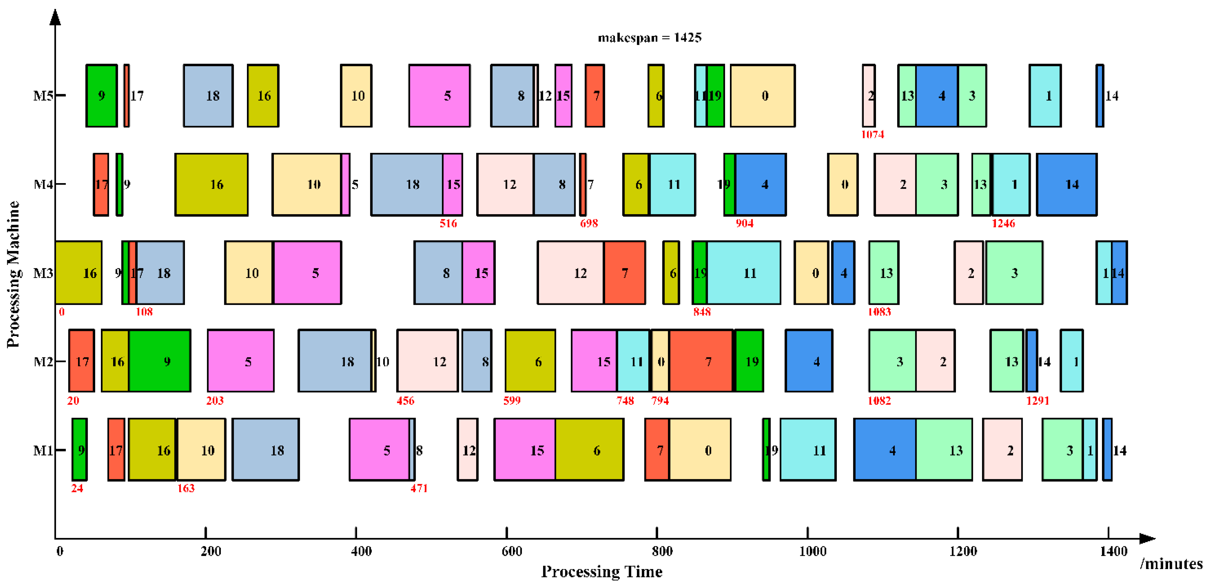
In addition, to illustrate the best scheduling results provided by the PBIG more clearly, Gantt charts are drawn in Figure 2 and Figure 3 for two instances, La11 and La12, respectively. In Figure 2 and Figure 3, we assume that time unit is minute, and the job number starts from zero. The start time of each job is marked as red. The processing times of all jobs are taken from the benchmark instances La11 and La12 (Lawrence [31]). For instance with La11, it can be seen from Table 4 that the best solutions obtained by the MCLM and HABC are 1635 and 1627, respectively. Compared with the MCLM and HABC, the PBIG can yield a solution with lower makespan value (1621). With La12, the PBIG can also yield a solution with lower makespan value than the MCLM and HABC.
5. Conclusions
This study considers the no-wait job shop scheduling problem by using a population-based iterated greedy (PBIG) algorithm. The problem is decomposed into a sequencing problem and timetabling problem. The Nawaz–Enscore–Ham (NEH) heuristic used for flow shop is extended in no-wait job shops, and an initialization scheme based on the NEH heuristic is developed to generate start solutions with both quality and diversity. Furthermore, a population-based co-evolutionary scheme is presented by imposing the iterated greedy procedure in parallel and hybridizing both the left timetabling and inverse left timetabling methods. Lastly, the proposed algorithm is compared with two effective metaheuristics in literature, and its effectiveness is demonstrated by computational results.
Considering the structural simplicity and high effectiveness of the PBIG, we hold the view that the algorithm is technically feasible to apply in practical production environment. In future, we will focus on adapting the PBIG algorithm for the multi-objective job shop scheduling problem, as well as the job shop scheduling problem with uncertainty.
Author Contributions
Conceptualization, G.D.; Formal analysis, S.Z.; Methodology, G.D.; Software, S.Z.; Supervision, G.D.; Validation, M.X.; Visualization, M.X.; Writing—original draft, M.X. All authors have read and agreed to the published version of the manuscript.
Funding
This research was funded by project ZR2019QF008 supported by Shandong Provincial Natural Science Foundation.
Institutional Review Board Statement
Not applicable.
Informed Consent Statement
Not applicable.
Data Availability Statement
The data presented in this study are available on request from the corresponding author.
Conflicts of Interest
The authors declare no conflict of interest.
References
- Pinedo, M. Scheduling: Theory, Algorithms, and Systems, 5th ed.; Springer: Berlin/Heidelberg, Germany, 2016. [Google Scholar]
- Tang, L.; Liu, J.; Rong, A.; Yang, Z. A mathematical programming model for scheduling steelmaking-continuous casting production. Eur. J. Oper. Res. 2000, 120, 423–435. [Google Scholar] [CrossRef]
- Grabowski, J.; Pempera, J. Sequencing of jobs in some production system. Eur. J. Oper. Res. 2000, 125, 535–550. [Google Scholar] [CrossRef]
- Rajendran, C. A no-wait flow shop scheduling heuristic to minimize makespan. Eur. J. Oper. Res. 1994, 45, 472–478. [Google Scholar]
- Hall, N.; Sriskandarajah, C. A survey of machine scheduling problems with blocking and no-wait in process. Oper. Res. 1996, 44, 510–525. [Google Scholar] [CrossRef]
- Lenstra, J.K.; Kan, A.H.G.R.; Brucker, P. Complexity of machine scheduling problems. Ann. Discret. Math. 1997, 1, 343–362. [Google Scholar]
- Sahni, S.; Cho, Y. Complexity of scheduling shops with no-wait in process. Math. Oper. Res. 1979, 4, 448–457. [Google Scholar] [CrossRef]
- Mascis, A.; Pacciarelli, D. Job-shop scheduling with blocking and no-wait constraints. Eur. J. Oper. Res. 2002, 143, 498–517. [Google Scholar] [CrossRef]
- Van den Broek, J. MIP-Based Approaches for Complex Planning Problems. Ph.D. Thesis, Technische Universiteit Eindhoven, Eindhoven, The Netherlands, 2009. [Google Scholar]
- Bürgy, R.; Gröflin, H. Optimal job insertion in the no-wait job shop. J. Comb. Optim. 2013, 26, 345–371. [Google Scholar] [CrossRef]
- Macchiaroli, R.; Mole, S.; Riemma, S. Modelling and optimization of industrial manufacturing processes subject to no-wait constraints. Int. J. Prod. Res. 1999, 37, 2585–2607. [Google Scholar] [CrossRef]
- Schuster, C.; Framinan, J. Approximate procedures for no-wait job shop scheduling. Oper. Res. Lett. 2003, 31, 308–318. [Google Scholar] [CrossRef]
- Schuster, C. No-wait job shop scheduling: Tabu search and complexity of subproblems. Math. Methods Oper. Res. 2006, 63, 473–491. [Google Scholar] [CrossRef]
- Framinan, J.M.; Schuster, C. An enhanced timetabling procedure for the no-wait job shop problem: A complete local search approach. Comput. Oper. Res. 2006, 331, 1200–1213. [Google Scholar] [CrossRef]
- Zhu, J.; Li, X.; Wang, Q. Complete local search with limited memory algorithm for no-wait job shops to minimize makespan. Eur. J. Oper. Res. 2009, 198, 378–386. [Google Scholar] [CrossRef]
- Zhu, J.; Li, X. An effective meta-heuristic for no-wait job shops to minimize makespan. IEEE Trans. Autom. Sci. Eng. 2012, 9, 189–198. [Google Scholar] [CrossRef]
- Mokhtari, H. A two-stage no-wait job shop scheduling problem by using a neuro-evolutionary variable neighborhood search. Int. J. Adv. Manuf. Technol. 2014, 74, 1595–1610. [Google Scholar]
- Aitzai, A.; Benmedjdoub, B.; Boudhar, M. Branch-and-bound and PSO algorithms for no-wait job shop scheduling. J. Intell. Manuf. 2016, 27, 679–688. [Google Scholar] [CrossRef]
- Li, X.; Xu, H.; Li, M. A memory-based complete local search method with variable neighborhood structures for no-wait job shops. Int. J. Adv. Manuf. Technol. 2016, 87, 1401–1408. [Google Scholar]
- Sundar, S.; Suganthan, P.N.; Jin, C.T.; Xiang, C.T.; Soon, C.C. A hybrid artificial bee colony algorithm for the job-shop scheduling problem with no-wait constraint. Soft Comput. 2017, 21, 1193–1202. [Google Scholar]
- Ruiz, R.; Stutzle, T. A simple and effective iterated greedy algorithm for the permutation flowshop scheduling problem. Eur. J. Oper. Res. 2007, 177, 2033–2049. [Google Scholar]
- Lee, C.H. A dispatching rule and a random iterated greedy metaheuristic for identical parallel machine scheduling to minimize total tardiness. Int. J. Prod. Res. 2018, 56, 2292–2308. [Google Scholar] [CrossRef]
- Ruiz, R.; Pan, Q.K.; Naderi, B. Iterated greedy methods for the distributed permutation fowshop scheduling problem. OMEGA 2019, 83, 213–222. [Google Scholar] [CrossRef]
- Ribas, I.; Companys, R.; Tort-Martorell, X. An iterated greedy algorithm for solving the total tardiness parallel blocking flow shop scheduling problem. Expert Syst. Appl. 2019, 121, 347–361. [Google Scholar] [CrossRef]
- Samarghandi, H.; ElMekkawy, T.Y.; Ibrahem, A.M. Studying the effect of different combinations of timetabling with sequencing algorithms to solve the no-wait job shop scheduling problem. Int. J. Prod. Res. 2013, 51, 4942–4965. [Google Scholar] [CrossRef]
- Deng, G.; Su, Q.; Zhang, Z.; Liu, H.; Zhang, S.; Jiang, T. A population-based iterated greedy algorithm for no-wait job shop scheduling with total flow time criterion. Eng. Appl. Artif. Intell. 2020, 88, 103369. [Google Scholar] [CrossRef]
- Nawaz, M.; Enscore, J.E.E.; Ham, I. A heuristic algorithm for the m-machine, n-job flow-shop sequencing problem. Omega 1983, 11, 91–95. [Google Scholar] [CrossRef]
- Fisher, H.; Thompson, G.L. Probabilistic Learning Combinations of Local Job-Shop Scheduling Rules. Industrial Scheduling; Prentice-Hall: Englewood Cliffs, NJ, USA, 1963; pp. 225–251. [Google Scholar]
- Applegate, D.; Cook, W. A computational study of the job-shop problem. ORSA J. Comput. 1991, 3, 149–156. [Google Scholar] [CrossRef]
- Adams, J.; Balas, E.; Zawack, D. The shifting bottleneck procedure for job shop scheduling. Manag. Sci. 1988, 34, 391–401. [Google Scholar] [CrossRef]
- Lawrence, S. Resource Constrained Project Scheduling: An Experimental Investigation of Heuristic Scheduling Techniques; Technical Report; Carnegie-Mellon University: Pittsburgh, PA, USA, 1984. [Google Scholar]
- Storer, R.H.; Wu, S.D.; Vaccari, R. New search spaces for sequencing instances with application to job shop scheduling. Manag. Sci. 1992, 38, 1495–1509. [Google Scholar] [CrossRef]
- Deng, G.; Zhang, Z.; Jiang, T.; Zhang, S. Total flow time minimization in no-wait job shop using a hybrid discrete group search optimizer. Appl. Soft Comput. 2019, 81, 105480. [Google Scholar] [CrossRef]
- Montgomery, D.C. Design and Analysis of Experiments, 8th ed.; Wiley: New York, NY, USA, 2012. [Google Scholar]
Figure 1.
Means plot for the parameters with least significant difference (LSD) 95% confidence intervals.
Figure 1.
Means plot for the parameters with least significant difference (LSD) 95% confidence intervals.

Figure 2.
Scheduling Gantt chart obtained by the PBIG for the instance La11.

Figure 3.
Scheduling Gantt chart obtained by the PBIG for the instance La12.


Table 1.
Notations used throughout the paper.
| Notation. | Description | Notation | Description |
|---|---|---|---|
| m | number of machines | ti | start time of Ji |
| n | number of jobs | job permutation | |
| M = {M1, M2, …, Mm} | set of m machines | t[i] | start time of |
| J = {J1, J2, …, Jn} | set of n jobs | operation of on | |
| oi,u | u-th operation of Ji | processing time of | |
| Mi,u | machine on which oi,u is processed | start time difference set | |
| pi,u | processing time of oi,u | makespan of | |
| Pi,u = | cumulated processing time of Ji when oi,u is finished | start time table of | |
| = {(u,v)| Mi,u = Mj,v} | pairs of operations processed on the same machine | cumulated processing time of when is finished | |
| Li | total processing times of Ji |
Table 2.
Analysis of variance (ANOVA) results for the calibration.
| Source | Sum of Squares | Df | Mean Square | F-Ratio | p-Value |
|---|---|---|---|---|---|
| MAIN EFFECTS | |||||
| A: p | 54.9931 | 3 | 18.3310 | 16.8500 | 0.0000 |
| B: d | 343.396 | 3 | 114.465 | 105.220 | 0.0000 |
| C: pb | 5.45246 | 3 | 1.81749 | 1.67000 | 0.1737 |
| D: D | 142.747 | 3 | 47.5825 | 43.7400 | 0.0000 |
| E: instance | 7962.73 | 6 | 1327.12 | 1219.90 | 0.0000 |
| REDIDUAL | 9797.72 | 8941 | 1.09582 | ||
| TOTAL (CORRECTED) | 18307.0 | 8959 |
Table 3.
Results for the modified complete local search with memory (MCLM), hybrid artificial bee colony (HABC) and population-based iterated greedy (PBIG) on the small instances.
Table 3.
Results for the modified complete local search with memory (MCLM), hybrid artificial bee colony (HABC) and population-based iterated greedy (PBIG) on the small instances.
| Instance. | n, m | BKS | MCLM | HABC | PBIG | ||||||
|---|---|---|---|---|---|---|---|---|---|---|---|
| RPDB | ARPD | TA(s) | RPDB | ARPD | TA(s) | RPDB | ARPD | TA(s) | |||
| Ft06 | 6, 6 | 73 | 0.00 | 0.00 | 0.00 | 0.00 | 0.00 | 0.15 | 0.00 | 0.00 | 0.65 |
| La01 | 10, 5 | 971 | 0.00 | 0.00 | 4.55 | 0.41 | 0.41 | 0.78 | 0.00 | 0.02 | 1.50 |
| La02 | 10, 5 | 937 | 0.00 | 0.00 | 7.60 | 2.56 | 2.56 | 1.41 | 0.00 | 0.00 | 1.50 |
| La03 | 10, 5 | 820 | 0.00 | 0.00 | 3.10 | 0.00 | 0.00 | 0.70 | 0.00 | 0.00 | 1.50 |
| La04 | 10, 5 | 887 | 0.00 | 0.00 | 6.25 | 0.00 | 0.00 | 0.87 | 0.00 | 0.00 | 1.50 |
| La05 | 10, 5 | 777 | 0.51 | 0.90 | 3.90 | 0.51 | 0.51 | 1.14 | 0.00 | 0.00 | 1.50 |
| Ft10 | 10, 10 | 1607 | 0.00 | 0.00 | 7.85 | 0.00 | 0.00 | 9.86 | 0.00 | 0.00 | 3.00 |
| Orb01 | 10, 10 | 1615 | 0.00 | 0.00 | 6.65 | 0.00 | 0.00 | 8.00 | 0.00 | 0.00 | 3.00 |
| Orb02 | 10, 10 | 1485 | 2.16 | 2.16 | 6.70 | 0.00 | 0.00 | 6.86 | 0.00 | 0.00 | 3.00 |
| Orb03 | 10, 10 | 1599 | 0.00 | 0.00 | 13.75 | 0.00 | 0.00 | 10.07 | 0.00 | 0.00 | 3.00 |
| Orb04 | 10, 10 | 1653 | 0.00 | 0.12 | 7.85 | 0.00 | 0.00 | 5.28 | 0.00 | 0.00 | 3.00 |
| Orb05 | 10, 10 | 1365 | 0.00 | 0.00 | 8.50 | 0.37 | 0.37 | 4.77 | 0.15 | 0.15 | 3.00 |
| Orb06 | 10, 10 | 1555 | 0.00 | 0.00 | 3.55 | 0.00 | 0.00 | 5.76 | 0.00 | 0.00 | 3.00 |
| Orb07 | 10, 10 | 689 | 0.00 | 0.00 | 7.25 | NA | NA | NA | 0.00 | 0.00 | 3.00 |
| Orb08 | 10, 10 | 1319 | 0.00 | 0.00 | 6.40 | 0.00 | 0.00 | 8.99 | 0.00 | 0.00 | 3.00 |
| Orb09 | 10, 10 | 1445 | 0.00 | 0.00 | 4.25 | 0.00 | 0.28 | 4.10 | 0.00 | 0.00 | 3.00 |
| Orb10 | 10, 10 | 1557 | 0.00 | 0.00 | 11.85 | 0.00 | 0.00 | 5.51 | 0.00 | 0.00 | 3.00 |
| La16 | 10, 10 | 1575 | 1.84 | 1.84 | 5.65 | 0.00 | 0.00 | 5.43 | 0.00 | 0.00 | 3.00 |
| La17 | 10, 10 | 1371 | 0.00 | 0.12 | 11.85 | 0.00 | 0.00 | 4.62 | 0.00 | 0.00 | 3.00 |
| La18 | 10, 10 | 1417 | 2.82 | 2.82 | 6.15 | 0.00 | 5.22 | 7.13 | 0.00 | 0.00 | 3.00 |
| La19 | 10, 10 | 1482 | 0.00 | 0.61 | 5.00 | 0.00 | 0.43 | 3.44 | 0.00 | 0.00 | 3.00 |
| La20 | 10, 10 | 1526 | 1.31 | 1.31 | 5.40 | 0.00 | 0.00 | 3.00 | 0.00 | 0.00 | 3.00 |
| Average | 0.39 | 0.45 | 6.55 | 0.23 | 0.47 | 4.63 | 0.01 | 0.01 | 2.55 | ||
Table 4.
Results for the MCLM, HABC and PBIG on the large instances.
| Instance | n, m | BKS | MCLM | HABC | PBIG | |||||||||
|---|---|---|---|---|---|---|---|---|---|---|---|---|---|---|
| Best | RPDB | ARPD | TA(s) | Best | RPDB | ARPD | TA(s) | Best | RPDB | ARPD | TA(s) | |||
| La06 | 15, 5 | 1248 | 1248 | 0.00 | 0.75 | 90.00 | 1248 | 0.00 | 0.00 | 39.99 | 1248 | 0.00 | 0.00 | 67.50 |
| La07 | 15, 5 | 1172 | 1178 | 0.51 | 2.46 | 83.00 | 1172 | 0.00 | 0.92 | 90.19 | 1172 | 0.00 | 0.44 | 67.50 |
| La08 | 15, 5 | 1244 | 1244 | 0.00 | 0.47 | 80.00 | 1244 | 0.00 | 0.15 | 85.63 | 1244 | 0.00 | 0.48 | 67.51 |
| La09 | 15, 5 | 1358 | 1365 | 0.52 | 0.73 | 106.00 | 1362 | 0.29 | 0.67 | 34.43 | 1362 | 0.29 | 0.61 | 67.50 |
| La10 | 15, 5 | 1287 | 1287 | 0.00 | 0.04 | 69.00 | 1294 | 0.54 | 0.70 | 65.42 | 1294 | 0.54 | 0.84 | 67.50 |
| La11 | 20, 5 | 1671 | 1635 | −2.15 | −0.58 | 439.00 | 1627 | −2.63 | −1.97 | 259.37 | 1621 | −2.99 | −1.08 | 120.02 |
| La12 | 20, 5 | 1452 | 1429 | −1.58 | 0.57 | 593.00 | 1434 | −1.24 | 0.00 | 168.97 | 1425 | −1.86 | 0.17 | 120.02 |
| La13 | 20, 5 | 1624 | 1605 | −1.17 | −0.15 | 303.00 | 1580 | −2.71 | −1.47 | 222.40 | 1582 | −2.59 | −0.09 | 120.02 |
| La14 | 20, 5 | 1691 | 1648 | −2.54 | −1.16 | 314.00 | 1640 | −3.02 | −2.24 | 156.58 | 1640 | −3.02 | −1.96 | 120.02 |
| La15 | 20, 5 | 1694 | 1685 | −0.53 | 1.09 | 424.00 | 1679 | −0.89 | −0.09 | 240.56 | 1677 | −1.00 | 0.35 | 120.02 |
| La21 | 15, 10 | 2048 | 2048 | 0.00 | 0.11 | 78.00 | 2043 | −0.24 | 0.27 | 71.42 | 2043 | −0.24 | −0.04 | 135.01 |
| La22 | 15, 10 | 1887 | 1902 | 0.80 | 0.99 | 142.00 | 1852 | −1.85 | −1.12 | 91.66 | 1852 | −1.85 | −1.19 | 135.01 |
| La23 | 15, 10 | 2032 | 2022 | −0.49 | 1.47 | 50.00 | 2032 | 0.00 | 0.71 | 120.56 | 2032 | 0.00 | 0.14 | 135.01 |
| La24 | 15, 10 | 2015 | 2015 | 0.00 | 0.77 | 98.00 | 1994 | −1.04 | −0.02 | 97.64 | 1994 | −1.04 | −0.30 | 135.01 |
| La25 | 15, 10 | 1917 | 1930 | 0.68 | 2.07 | 71.00 | 1906 | −0.57 | −0.57 | 92.53 | 1906 | −0.57 | −0.57 | 135.01 |
| La26 | 20, 10 | 2553 | 2532 | −0.82 | 1.91 | 349.00 | 2506 | −1.84 | 0.30 | 223.46 | 2506 | −1.84 | 1.66 | 240.02 |
| La27 | 20, 10 | 2747 | 2715 | −1.17 | 0.28 | 388.00 | 2674 | −2.66 | −2.62 | 154.83 | 2673 | −2.69 | −2.19 | 240.02 |
| La28 | 20, 10 | 2624 | 2560 | −2.44 | 1.77 | 313.00 | 2560 | −2.44 | 0.62 | 197.33 | 2581 | −1.64 | 0.77 | 240.03 |
| La29 | 20, 10 | 2489 | 2367 | −4.90 | −2.48 | 445.00 | 2389 | −4.02 | −2.70 | 531.94 | 2405 | −3.37 | −2.18 | 240.03 |
| La30 | 20, 10 | 2665 | 2544 | −4.54 | −1.51 | 376.00 | 2452 | −7.99 | −3.00 | 248.25 | 2452 | −7.99 | −3.50 | 240.03 |
| La31 | 30, 10 | 3745 | 3575 | −4.54 | −1.40 | 3099.00 | 3592 | −4.09 | −2.60 | 1716.18 | 3479 | −7.10 | −2.35 | 540.16 |
| La32 | 30, 10 | 4028 | 3835 | −4.79 | 0.56 | 3314.00 | 3913 | −2.86 | −0.35 | 1590.40 | 3877 | −3.75 | −0.68 | 540.19 |
| La33 | 30, 10 | 3749 | 3574 | −4.67 | −1.52 | 3003.00 | 3529 | −5.87 | −3.37 | 1544.34 | 3560 | −5.04 | −2.51 | 540.18 |
| La34 | 30, 10 | 3824 | 3684 | −3.66 | −0.88 | 3375.00 | 3610 | −5.60 | −2.76 | 1405.05 | 3615 | −5.47 | −2.55 | 540.20 |
| La35 | 30, 10 | 3760 | 3698 | −1.65 | 1.27 | 3083.00 | 3593 | −4.44 | −0.41 | 1797.55 | 3687 | −1.94 | 0.43 | 540.19 |
| La36 | 15, 15 | 2685 | 2736 | 1.90 | 4.98 | 189.00 | 2685 | 0.00 | 0.29 | 76.42 | 2685 | 0.00 | 0.00 | 202.51 |
| La37 | 15, 15 | 2962 | 2962 | 0.00 | 0.11 | 93.00 | 2938 | −0.81 | 0.98 | 184.41 | 2831 | −4.42 | 0.06 | 202.51 |
| La38 | 15, 15 | 2617 | 2525 | −3.52 | −1.73 | 91.00 | 2525 | −3.52 | −1.08 | 311.66 | 2525 | −3.52 | −2.80 | 202.51 |
| La39 | 15, 15 | 2697 | 2729 | 1.19 | 2.43 | 116.00 | 2703 | 0.22 | 0.88 | 146.87 | 2687 | −0.37 | 0.34 | 202.51 |
| La40 | 15, 15 | 2594 | 2580 | −0.54 | −0.54 | 61.00 | 2594 | 0.00 | 0.00 | 190.51 | 2594 | 0.00 | 0.00 | 202.51 |
| Swv01 | 20, 10 | 2328 | 2333 | 0.22 | 0.37 | 516.00 | 2318 | −0.43 | −0.02 | 874.70 | 2318 | −0.43 | −0.17 | 240.02 |
| Swv02 | 20, 10 | 2418 | 2418 | 0.00 | 0.38 | 488.00 | 2417 | −0.04 | −0.02 | 961.12 | 2417 | −0.04 | −0.02 | 240.02 |
| Swv03 | 20, 10 | 2415 | 2381 | −1.41 | −0.41 | 517.00 | 2381 | −1.41 | −0.92 | 1018.02 | 2381 | −1.41 | −0.89 | 240.02 |
| Swv04 | 20, 10 | 2506 | 2462 | −1.76 | −0.30 | 426.00 | 2506 | 0.00 | 0.29 | 1728.64 | 2462 | −1.76 | −0.10 | 240.02 |
| Swv05 | 20, 10 | 2333 | 2333 | 0.00 | 0.00 | 285.00 | 2333 | 0.00 | 0.00 | 535.69 | 2333 | 0.00 | 0.00 | 240.02 |
| Swv06 | 20, 15 | 3291 | 3291 | 0.00 | 1.69 | 747.00 | 3291 | 0.00 | 0.40 | 885.67 | 3291 | 0.00 | 0.05 | 360.02 |
| Swv07 | 20, 15 | 3271 | 3219 | −1.59 | −0.95 | 584.00 | 3188 | −2.54 | −2.54 | 829.20 | 3188 | −2.54 | −2.43 | 360.01 |
| Swv08 | 20, 15 | 3530 | 3423 | −3.03 | −2.21 | 413.00 | 3423 | −3.03 | −1.78 | 1150.09 | 3423 | −3.03 | −2.56 | 360.02 |
| Swv09 | 20, 15 | 3307 | 3270 | −1.12 | −0.28 | 448.00 | 3246 | −1.84 | −0.86 | 1531.08 | 3246 | −1.84 | −1.12 | 360.02 |
| Swv10 | 20, 15 | 3488 | 3451 | −1.06 | 0.12 | 520.00 | 3462 | −0.75 | −0.22 | 1425.36 | 3462 | −0.75 | −0.64 | 360.02 |
| Average | −1.25 | 0.28 | 654.48 | −1.73 | −0.64 | 577.40 | −1.88 | −0.64 | 238.16 | |||||
Publisher’s Note: MDPI stays neutral with regard to jurisdictional claims in published maps and institutional affiliations. |
© 2021 by the authors. Licensee MDPI, Basel, Switzerland. This article is an open access article distributed under the terms and conditions of the Creative Commons Attribution (CC BY) license (https://creativecommons.org/licenses/by/4.0/).
Share and Cite
MDPI and ACS Style
Xu, M.; Zhang, S.; Deng, G. No-Wait Job Shop Scheduling Using a Population-Based Iterated Greedy Algorithm. Algorithms 2021, 14, 145. https://0-doi-org.brum.beds.ac.uk/10.3390/a14050145
AMA Style
Xu M, Zhang S, Deng G. No-Wait Job Shop Scheduling Using a Population-Based Iterated Greedy Algorithm. Algorithms. 2021; 14(5):145. https://0-doi-org.brum.beds.ac.uk/10.3390/a14050145
Chicago/Turabian StyleXu, Mingming, Shuning Zhang, and Guanlong Deng. 2021. "No-Wait Job Shop Scheduling Using a Population-Based Iterated Greedy Algorithm" Algorithms 14, no. 5: 145. https://0-doi-org.brum.beds.ac.uk/10.3390/a14050145
Note that from the first issue of 2016, this journal uses article numbers instead of page numbers. See further details here.