
Approximately Optimal Control of Nonlinear Dynamic Stochastic Problems with Learning: The OPTCON Algorithm


Department of Economics, University of Klagenfurt, 9020 Klagenfurt, Austria
*
Author to whom correspondence should be addressed.
Algorithms 2021, 14(6), 181; https://0-doi-org.brum.beds.ac.uk/10.3390/a14060181
Submission received: 31 March 2021
/
Revised: 31 May 2021
/
Accepted: 4 June 2021
/
Published: 8 June 2021
(This article belongs to the Special Issue Stochastic Algorithms and Their Applications)
Abstract
:OPTCON is an algorithm for the optimal control of nonlinear stochastic systems which is particularly applicable to economic models. It delivers approximate numerical solutions to optimum control (dynamic optimization) problems with a quadratic objective function for nonlinear economic models with additive and multiplicative (parameter) uncertainties. The algorithm was first programmed in C# and then in MATLAB. It allows for deterministic and stochastic control, the latter with open loop (OPTCON1), passive learning (open-loop feedback, OPTCON2), and active learning (closed-loop, dual, or adaptive control, OPTCON3) information patterns. The mathematical aspects of the algorithm with open-loop feedback and closed-loop information patterns are presented in more detail in this paper.
1. Introduction
Optimal control of stochastic processes is a topic which occurs in many contexts of applied mathematics such as engineering, biology, chemistry, economics, and management science. These techniques are used to steer the behavior of a plant, natural, human or social system over a certain (finite or infinite) time period where the system is driven by differential or difference equations whose time path can be influenced by an external controller. The controller (decision maker, policy maker) aims at achieving the best trajectory of his/her controls according to some criterion (performance measure, objective function) over that time horizon.
Unfortunately, only a few special cases can be solved explicitly, in particular the linear-quadratic-Gaussian problem, where the dynamic system is linear, the objective function is quadratic, and the stochastics are confined to additive normally distributed noise affecting the system dynamics (e.g., [1]). In this case, it is possible to separate the estimation of the state and the optimization of its behavior due to the property of certainty equivalence (the separation theorem). For most practical applications, however, especially those where the parameters of the system are not known precisely, an exact solution to the optimal stochastic control problem is not available and some kind of approximation is required. One of the reasons is the curse of dimensionality, which prevents the solving of dynamic functional equations for multivariable systems [2,3]. This is particularly complicated by the so-called dual effect of controls preventing the separation of estimation and control in adaptive processes; it was discovered by [4] that “the control must have a reciprocal, ‘dual’ character: to a certain extent they must be of a probing nature, but also controlling to a known degree” ([4], p. 31). The dynamic functional equations for general problems of this kind are known (see, e.g., [5]) but cannot be solved except in very special cases; hence approximations are required (see [6,7,8]).
In this paper, we present the OPTCON algorithm for calculating numerically (approximately) optimal control solutions to nonlinear dynamic stochastic optimization problems without and with learning. The algorithm was developed in three stages (OPTCON1, OPTCON2, and OPTCON3) over a long period. OPTCON1 determines optimal controls for deterministic problems and stochastic problems based on the open-loop information pattern [9]. OPTCON2 solves problems with passive learning about the unknown parameters of the system model [10], so-called open-loop feedback policies (see [11] for the terminology). Finally, OPTCON3 also includes active learning (dual, adaptive control) according to an approximation procedure initiated by [12,13,14], and adapted to linear economic systems by [15,16], cf. [17]. The present paper provides mathematical details for OPTCON3, which is the most sophisticated version of the OPTCON algorithm; in [18] we concentrate on computations aspects and applications of OPTCON3.
The OPTCON algorithm is applicable for stochastic control problems with the following properties: The model of the process is multivariable, formulated in discrete time, and described by a system of nonlinear difference equations with known functional form but additive noise and (possibly) unknown parameters. The state is stochastically observable and controllable. No inequality constraints on states or controls are given. Open-loop, open-loop feedback, and closed-loop information structures can be considered. The objective function is quadratic and perfectly known; it is formulated in tracking form but can easily be transformed to the general quadratic form. Quadratic functions can be interpreted as second-order Taylor approximations to more general functional forms. There is only one decision maker; for decentralized problems, see the OPTGAME algorithm [19].
The paper has the following structure. In Section 2 the relevant basic background is provided, namely the class of problems to be solved by the algorithm as well as some basic information about the linear-quadratic framework and nonlinear system solving algorithms. Section 3 presents the OPTCON algorithm stepwise, starting with the basic version (OPTCON1) and then introducing the more advanced versions OPTCON2 and OPTCON3 for handling stochastic components in the optimal control process. In Section 4 some details on computational time and accuracy of the OPTCON algorithm are presented. Section 5 concludes.
2. Theoretical Background
2.1. Optimal Control Problem
We consider optimal control problems with a quadratic objective function and a nonlinear multivariate discrete-time dynamic system under additive and parameter uncertainties. The basis for an optimal control problem is a deterministic dynamic system to be controlled (plant, firm, economy, etc.) in discrete time in the form:
where:
- -
- is a vector of state variables that describes the state of the system at any point in time t,
- -
- is a vector of control variables; we assume that the decision maker determines the values of the control variables exactly (without randomization) according to the approximately optimal solution of the problem,
- -
- denotes a vector of non-controlled deterministic exogenous variables, whose values are known to the decision maker at time t,
- -
- T denotes the terminal time period of the finite planning horizon.
The function f is assumed to be twice continuously differentiable with respect to all of its arguments.
We assume that there is some true law of motion given by Equation (1) in the background which is at least partially unknown to the policy maker while the function f is known to him/her. The policy maker faces two sources of uncertainty, additive and parameter uncertainties where:
- -
- denotes a vector of stochastic variables of system parameters (parameter uncertainty),
- -
- is a vector of true parameters whose values are assumed to be constant but unknown to the policy maker,
- -
- is a vector of additive stochastic disturbances (system error).
and are assumed to be independent Gaussian random vectors with expectations and respectively and covariance matrices and respectively.
Including uncertainty, the system (1) can be written as:
The optimal control problem to be solved approximately assumes that there is a modeler who wishes to control the system (2). It means that the controller wishes to bring the state variables, using the control variables, as close as possible to some pre-defined desired time path, according to a given optimality criterion. The OPTCON algorithm allows for the optimal control of the system (2) using a quadratic objective function. To this end the modeler needs to define the following variables:
- -
- are given target (‘ideal’) values (for ) of the state variables,
- -
- are given target (‘ideal’) values (for ) of the control variables,
- -
- is an symmetric matrix defining the relative weights of the state and control variables in the objective function. In a frequent special case, includes a discount factor with .
The resulting intertemporal objective function is given in quadratic tracking form:
with
2.2. Linear-Quadratic Optimal Control (LQ) Framework
The novel feature of the OPTCON algorithm is the combination of a nonlinear dynamic system and the above-mentioned stochastics when solving optimal control problems. Before we can discuss this technique in detail, a few words should be said about the underlying linear-quadratic optimal control framework. The dynamic system is given in linear form as
The corresponding optimal control objective function can be written in the same form as in (3) and (4). Using well-known LQ optimization techniques, the rules for defining control variables can be found iteratively backwards in time using dynamic Riccati equations. We start from the familiar LQ framework (e.g., [20]), which was adapted to economic models by [15,21,22]. The same standard technique is applied in the OPTCON algorithm whenever an optimal control for a linearized system should be obtained.
2.3. Solving Nonlinear Dynamic Systems
The OPTCON algorithm allows us to find approximately optimal control solutions for nonlinear stochastic systems. In the solution process, the nonlinear dynamic system (2) should be solved in a large number of iterations. For this reason the choice of an appropriate solver is important to guarantee obtaining reliable solutions taking the computational costs into account. In the OPTCON algorithm, different solution algorithms are included attaching different importance to the trade-off between reliability and computational speed. At the moment the following methods can be used: Levenberg–Marquardt [24], trust region [25], Newton–Raphson [26], or Gauss–Seidel [27].
3. The OPTCON Algorithm
3.1. The OPTCON1 Algorithm
The first version of the OPTCON algorithm, the OPTCON1 algorithm, was developed by [9]. It allows us to calculate an open-loop (OL) solution to a nonlinear stochastic dynamic optimal control problem with a quadratic objective function under additive and parameter uncertainties. Open-loop controls either do not take account of the effect of uncertainties in the system or assume the stochastics (expectation and covariance matrices of additive and multiplicative disturbances) to be given for all time periods at the beginning of the planning horizon. The basic idea behind this algorithm is that it extends linear-quadratic stochastic optimal control techniques (see, e.g., [1]) to nonlinear problems using an iterative method of linear approximations.
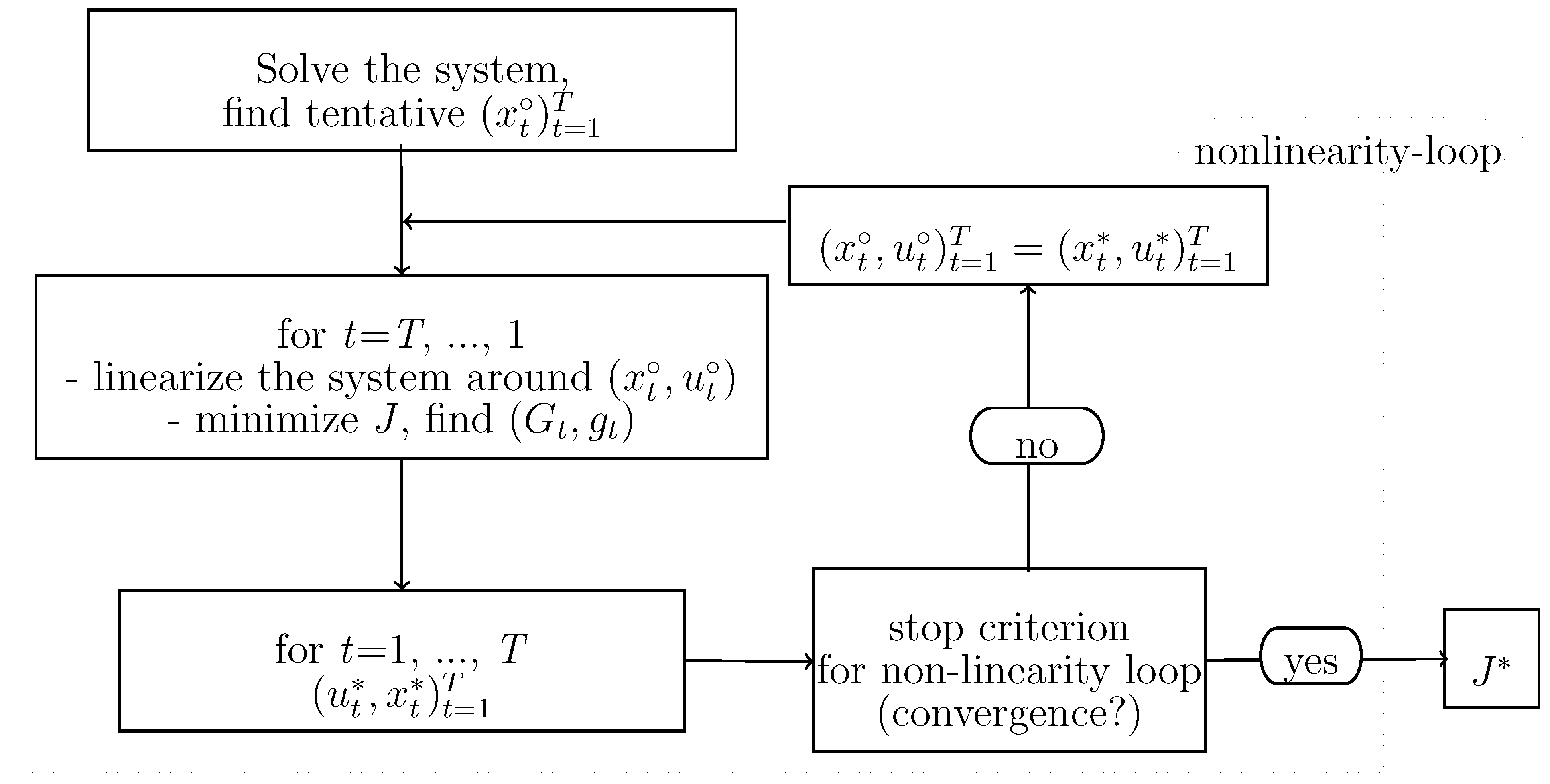
The OPTCON algorithm solves the nonlinear optimal control problem iteratively by a sequence of linear approximations where the next approximation is derived using the optimal control solution of the previous one. The (optimal) solutions of the intermediate linear approximations are iterated from one time path to another until the algorithm converges. The criterion for convergence is that the difference in the values of the state and control variables of current and previous iterations is smaller than a pre-specified number. or the maximal number of iterations is reached. In each iteration the same procedure is conducted, namely linearizing and optimizing the linearized system. The system is linearized around the previous iteration’s result and the problem is solved for the resulting time-varying linearized system. The solution of the linearized model is obtained via Bellman’s principle of optimality and is used as the tentative path for the next iteration, starting off the procedure all over again. If the OPTCON algorithm converges, the solution of the last iteration is taken as the approximately optimal solution to the nonlinear problem and the value of the objective function is calculated. Figure 1 shows the structure of the OPTCON1 algorithm.
3.2. The OPTCON2 Algorithm
The second version of the algorithm (called OPTCON2, see [10,23] for more details) extends the first version with a passive learning strategy (open-loop feedback (OLF)). OLF uses the idea of re-estimating the model at the end of each time period . For that purpose, the model builder (policy maker) observes the current situation and uses the new information, namely the current values of the state variables, to improve his/her knowledge of the system.
Recall that the stochastic system includes two kinds of uncertainties, namely additive (random system errors) and multiplicative (‘structural’ errors in parameters). We assume that there is some true law of motion in the background which is unknown to the policy maker. The passive learning strategy deals with the ‘true’ parameters which generate the model. However, the policy maker does not know these true parameters and works with the ‘wrong’ estimated parameters . The idea of the OLF strategy is to observe the outcome of the model in each time period and use this information to bring the estimated parameters closer to the true values .
The OLF strategy of the OPTCON2 algorithm consists of the following (rough) steps running in a forward loop.
In each time period S () do the following:
- Find an (approximately) optimal open-loop solution for the remaining subproblem (for the time periods from S to T) using the OPTCON1 algorithm.
- Fix the predicted solution for time period S, namely and .
- Observe the realized state variables which result from the chosen control variables (), the true law of motion with parameter vector , and the realization of the random disturbances . The main difference between and is that the former is driven by the true dynamic process with parameter vector and the latter by the estimated dynamic system with .
- Update the parameter estimate (via the Kalman filter and using the difference between and ) and use it in the next iteration step .
The last step is carried out using the idea of the Kalman filter (see, e.g., [28] or [29]). The updating procedure according to the Kalman filter consists of two distinct phases, prediction and correction. First (the prediction phase), the predicted values of the state variables , the vector of parameters , and the covariances of the parameters are calculated using the estimates from the previous time period. Next (the correction phase), these ‘a priori’ values of the state variables, the vector of the parameters, and the values of the covariances are corrected using the current observations of the state variables.
The phase of calculating the predicted values of and is integrated in the previous steps of the OPTCON2 algorithm. At the end of time period S the predicted values of are calculated and is known.
The correction phase is reduced to the calculation of the parameter estimates and the parameter covariances because the ‘corrected’ values of the state variables are calculated in the previous step of the algorithm or simply observed. As explained before, the updating procedure is based on the difference between and at the end of each time period.
The OPTCON2 algorithm allows us to find an approximate solution of the optimal control problem using a passive learning strategy. The policy maker uses real observations in each time period to update his/her knowledge about the stochastic dynamic system. In many cases it allows him/her to obtain more reliable results (see [30] for a performance study on optimal control with a passive learning strategy).
3.3. The OPTCON3 Algorithm
In this section we present the detailed description of the OPTCON3 algorithm. As mentioned above, the latest version of the OPTCON algorithm includes an active learning strategy. In the literature this strategy is also called closed-loop, adaptive, or dual control. The passive learning method in the OPTCON2 algorithm uses current observations to update the information about the dynamic system. The active learning strategy in OPTCON3 actively uses system perturbations to improve the optimal control performance by reducing the uncertainty in the future.
The procedure for finding the closed-loop solution in the OPTCON3 algorithm is based on the linear active learning control method in [15]. Similar to the iterative structure in the OPTCON2 algorithm, the optimization runs in a forward loop (). However, in each time period, more information about future measurements is used. To this end the objective function J (as defined in Equations (3) and (4)) is extended for stochastic components. We define in each time period as the approximate total cost-to-go with periods remaining. The approximate cost-to-go is broken down into three terms: . is called deterministic term and incorporates only non-stochastic components. is the cautionary factor that includes the stochastic elements in the current period. is called probing term and captures the effect of dual learning on the uncertainty in the future periods. and constitute a separate quadratic minimization problem constrained by the nonlinear system. The original system needs to be expanded to the perturbation form . The optimization problem has to be solved for the perturbed system, where is the perturbed objective function. Using Taylor expansion of nonlinear system and Bellman optimization technique, we obtain the solution as a quadratic function of . The original can be derived from . To take uncertain parameters into account, all the terms and formulas need to be adjusted to the augmented system .
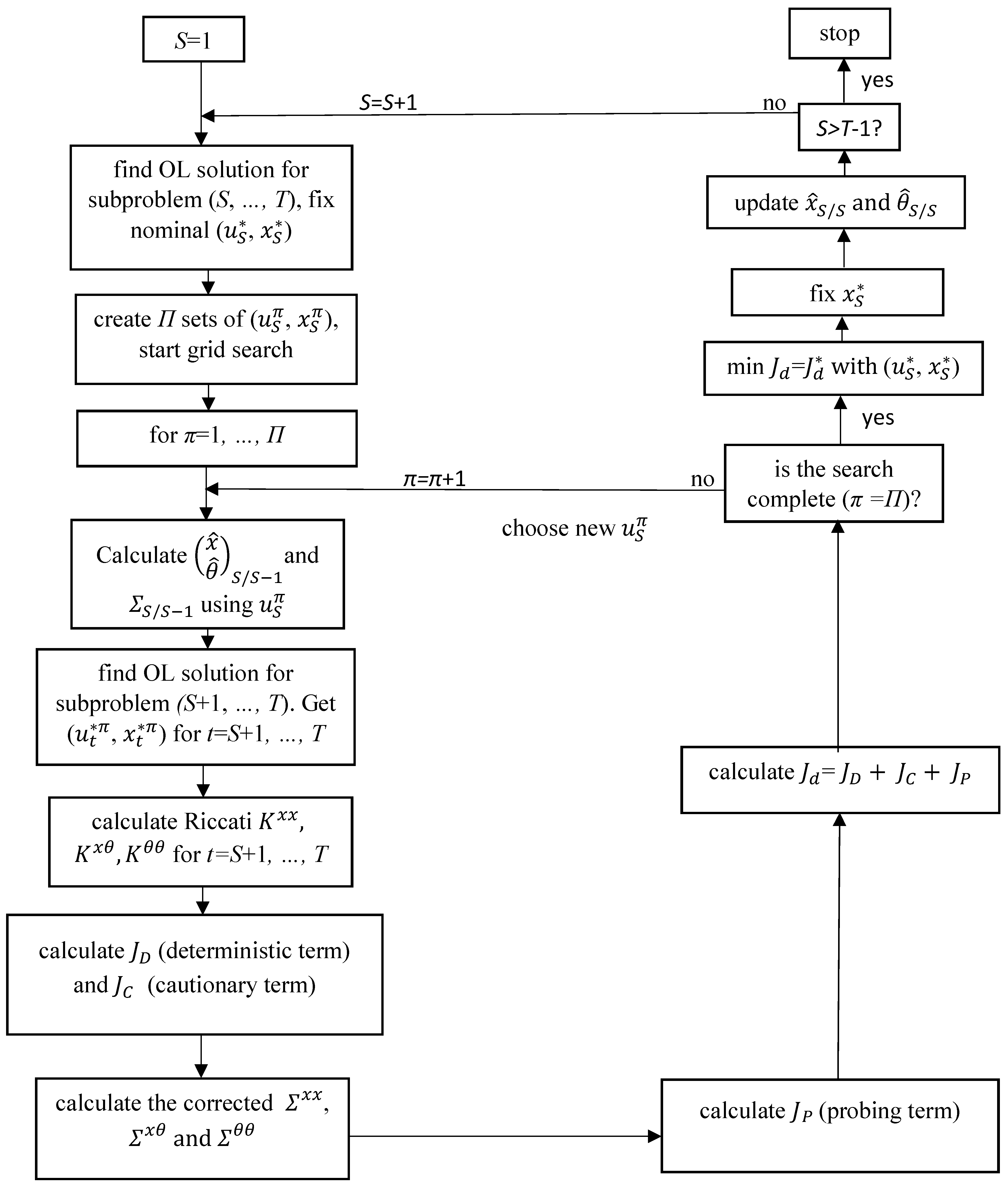
Next, a schematic structure of the OPTCON3 algorithm is presented. This structure is visualized in Figure 2.
The optimization is carried out in a forward loop from 1 to T conducting following procedure in each time period S (). The subproblem from S to T is solved via the open-loop (OL) strategy (see Figure 1 in Section 3.1). The OL solution for the time period S is fixed. After that the core part of the dual control strategy starts, where the system is actively perturbed to learn about it in order to minimize the uncertainty and the objective function values in the future. In the OPTCON3 algorithm a grid search method is used (instead of grid search many other methods can be applied, such as gradient optimization or a more advanced heuristic approach). In the so-called “-loop” we create a grid of possible solutions around the existing path . In each iteration (), i.e., in each grid point, the optimal control solution is obtained and evaluated using the objective function. Inside the -loop (for each ), the following steps are carried out.
An optimal open-loop solution for the subproblem from to T is determined. Then the OL solution for the time period is fixed. Next, after some auxiliary calculations (including, among other, Riccati matrices), the deterministic , cautionary , and probing terms of the cost-to-go are determined in a forward loop from to T. Once the iteration of the -loop has been completed, the total approximate objective function can be obtained. When the search is completed, i.e., the approximately optimal path with has been found, the obtained optimal control in time period is carried out by the policy maker. As a result of these controls and the true dynamic systems the actual values of the state variables can be obtained. This new information is used by the policy maker to update and to adjust the parameter estimate , whereby the Kalman filter is used. Using the updated stochastic parameters, the same active learning procedure is applied for the remaining time periods from to T.
The OPTCON3 algorithm basically uses the technique presented in [13,15] but is augmented by approximating, in each step, the nonlinear system in a series of linear systems (iterative procedure as described in Section 3.1).
The following steps (I–IV) of the OPTCON3 algorithm describe how to obtain an approximately optimal dual control solution to a stochastic problem.
The algorithm needs the following input values (A legitimate question would be how to obtain the required (tentative) inputs. It obviously depends on the research question. In the case of some numerical experiments, one can resort to Monte Carlo simulations. In the case of a real-world application, one can estimate system parameters by an appropriate method or simply guess some values):
| f | system function |
| initial values of state variables | |
| tentative path of control variables | |
| expected values of system parameters | |
| covariance matrix of system parameters | |
| covariance matrix of system noise | |
| system noises | |
| path of exogenous variables | |
| target path for state variables | |
| target path for control variables | |
| , , | weighting matrices of objective function |
| , | weighting vectors of objective function |
| discount factor of objective function. |
As a result of the algorithm, an approximately optimal solution , and the corresponding value of the objective function are obtained.
Step I: Do the following search steps [1], [2] and [3] for each :
Step I-[1]: Find the OL solution for the subproblem : apply the procedure already used in OPTCON1. Fix .
Step I-[2]: Run a grid search of size around , i.e., perform steps (A)–(G) for each :
Step I-2A: Find the OL solution for the subproblem (, …, T).
• The nonlinearity loop is run until the stop criterion is fulfilled (the stop criterion is fulfilled when the difference between the values of the current and the previous iteration is smaller than a pre-specified number or the maximum number of iterations is achieved). As a result the approximately optimal solution has been found. Then go to the next step I-2B.
Notes:
- -
- After several runs of the nonlinearity loop, only the solution ( for the time period will be taken as the optimal (nominal) solution. The calculations of the pairs for other periods ( > ) have to be done again, taking into account the re-estimated parameters for all periods.
- -
- After linearization the parameter matrices for the linearized system are obtained: and , where , , and are the derivatives of the system function f with respect to , , and respectively.
Step I-2B: Do a backward recursion to obtain auxiliary matrices for calculating components of the objective function.
Initialize the following auxiliary matrices for backward recursion:
Calculate the Riccati matrices , , and and the auxiliary matrices , , , , , , , , and backwards in time from T to .
where .
is the derivative of the system function with respect to .
Step I-2C: Calculate the deterministic component of the approximate objective function and the cautionary component :
Step I-2D: Repeat steps [a]–[c] for each :
- [a]:
- Calculate the components and :
- [b]:
- Calculate the matrix :with
- [c]:
- Compute the probing component :
Step I-2E: Calculate the sum of the deterministic, cautionary, and probing terms over the periods :
Step I-2F: Take a new control (a new point in the grid search) and go to step I-2A.
Step I-[3]: Choose an optimal with . End of grid search. Fix the corresponding .
Step II: Calculate the following (a) and (b) for only one time period S:
- (a)
- (b)
Step III: Update the parameter estimates and :
Step IV: Set and , go to Step I and run the procedure for the time period .
The OPTCON3 algorithm is finished when and the approximately optimal dual control and state variables have been found for all periods.
3.4. Computational Details for the AL Procedure
This subsection includes the technical computations for the AL procedure of the OPTCON3 algorithm.
The basic tasks are applying Bellman’s principle of optimality, linearization of the nonlinear system in perturbation form, minimizing the objective function, and inserting the obtained feedback rule for controls back into the objective function. In this way the (temporary) components of the optimal objective function can be derived. After that, due to the stochastic nature of the parameters (), all the components have to be adjusted to the extended system .
For use the (Taylor) series expansion:
where , are the gradients and , , and are the Hessian matrices; , , and is a nominal path.
Thus,
and
Next, apply the Taylor expansion to the nonlinear system, i.e., linearize the system function f in (2) around the reference values:
This can be rewritten in perturbation form:
Next, we have to prove that the term (21) can be expressed in the quadratic form as a function of only.
Assume
and apply the method of induction. By doing so the parameters g, and H are determined.
The next step is to prove that rule (23) is also true for .
Start with
By second order expansion we get:
Use and assumption (23)
Taking expectations over yields
Put (22) into (24) and set
Then by taking expectations over
The terms which are higher than second order are dropped here.
Then use the following notations:
and get
Apply the rule and take expectations over :
where .
Define
Note that because . Moreover . Thus,
Use the following rule:
and get
Defining
and
we get
This shows that is a quadratic function of .
Next, using the results of [31] we find the solution of the g recursion:
Let us define a deterministic term and a stochastic term , so that . By working backwards from period T the following can be shown:
Next, solve it partially for the stochastic term . For that define with .
Using again the backward recursion get the equation:
Then
where .
and
.
Then
This objective function can be split into three parts:
deterministic:
cautionary:
probing:
In this way the optimal control problem is solved and the components of the objective function are found. However, these are not the final results. In the next step, the stochastic parameters have to be taken into account, i.e., the extension of the system has to be considered.
3.5. Extension of the System
Recall that the algorithm deals with a quadratic criterion function when the parameters of the system equations are unknown. One technique to incorporate the uncertain parameters is to treat the random parameters as additional state variables.
Thus, apply the equations of the objective function to the system
Then
and
In order to calculate the adjusted components of the objective function (especially (40) and (41)) we need the terms H and .
First, we calculate the adapted using Definition (30):
where
and
We know that , , , and . Then we get
Define
Then using and we get the following:
Use the definition and get the following:
For the calculation of H we need the term :
Now we can calculate the term H for the extended system:
Thus,
After that we go back to the components of the objective function. According to (41) we need to calculate the term .
Thus,
Next we calculate . According to (40) we need to calculate and :
Thus,
Under the assumption (Kendrick (1981), Appendix J) the deterministic term is
where is a nominal path.
In order to calculate the components of the objective function we need to determine one more term, .
Use
where , , , .
Use the linearized system, i.e., apply:
, ,
and
4. Computational Aspects
In this paper we concentrate on mathematical details of the OPTCON algorithm. However, it is important to mention the computational characteristics of this algorithm. In order to show computational time and accuracy we used two different models: the MacRae model and the ATOPT model. As it would go beyond the scope of the present paper, we do not discuss these models and their economic interpretation (see detailed descriptions in [18]) but provide computational details of applying different versions of the OPTCON algorithm. We compared four different optimization strategies: deterministic solution (det), stochastic open-loop solution (OL) as described in Section 3.1, stochastic passive learning solution (OLF) as described in Section 3.2, and stochastic active learning solution (AL) as described in Section 3.3. In the case of the active learning strategy, a grid search with 100 grid points for each control variable was applied (see parameter in Step-I-[2] in Section 3.3). All calculations were performed on a Windows 10 computer with 16 GB RAM. The OPTCON algorithm is programmed in MATLAB (MATLAB R2020a); the MATLAB computer code is available on request.
The MacRae model is a simple linear model with one state and one control variable. One parameter is stochastic and the optimal control was calculated for two periods only. Table 1 summarizes the computational performance of the OPTCON algorithm for the MacRae model. In the case of a linear-quadratic deterministic optimal control framework convergence can be shown analytically. This is true for the MacRae model, at least for the deterministic and the OL case. Moreover, as a check for the special case of a linear system, we compared the results of OPTCON with those of the same model calculated by available software and found them to be the same apart from round-off errors.
The ATOPT model is a small nonlinear model consisting of three equations, one control variable, and two stochastic parameters. The optimal control is calculated for five periods. Table 1 summarizes the computational performance of the OPTCON algorithm for the MacRae model. Table 2 summarizes the computational performance of the OPTCON algorithm for the ATOPT model.
5. Concluding Remarks
In this paper, we described the OPTCON algorithm for the approximately optimal control of stochastic processes under a quadratic objective function. For systems with complete information, either deterministic or stochastic with known statistical characteristics of the disturbances, the open-loop version of OPTCON1 is suitable. OPTCON2 assumes partial information, in particular uncertain parameters of the system, with passive storage of information accruing during the control horizon, i.e., not used for control purposes. If active storage of information is possible, the dual control policy of OPTCON3 is appropriate. All three versions of OPTCON were programmed first in C# and then in MATLAB. We have applied OPTCON1 to various economic policy problems ([32,33], among others); Monte Carlo experiments with OPTCON2 and OPTCON3 have also yielded satisfactory results in terms of computing time. The results of approximately optimal policies were also as expected from the point of view of the economic problems under consideration. Due to the numerical nature of the algorithm, we cannot prove convergence in general; however, no problems of non-convergence have occurred so far. For future research, more applications are desirable to gain more insight into the different policies resulting from the various assumptions about the information structure of adaptive stochastic policy problems.
Author Contributions
Conceptualization, R.N., D.B. and V.B.-N.; methodology, V.B.-N., R.N. and D.B.; software, D.B.; formal analysis, V.B.-N.; writing—original draft preparation, V.B.-N., D.B. and R.N.; writing—review and editing, R.N., D.B. and V.B.-N.; visualization, D.B. and V.B.-N.; supervision, R.N.; funding acquisition, V.B.-N. All authors have read and agreed to the published version of the manuscript.
Funding
This research was funded by the Austrian Science Fund FWF (grant T 1012-GBL).
Conflicts of Interest
The authors declare no conflict of interest.
References
- Athans, M. The role and use of the stochastic linear-quadratic-Gaussian problem in control system design. IEEE Trans. Autom. Control 1971, 16, 529–552. [Google Scholar] [CrossRef]
- Bellman, R. Dynamic Programming; Princeton University Press: Princeton, NJ, USA, 1957. [Google Scholar]
- Bellman, R. Adaptive Control Processes: A Guided Tour; Princeton University Press: Princeton, NJ, USA, 1961. [Google Scholar]
- Fel’dbaum, A.A. Optimal Control Systems; New York Academic Press: New York, NY, USA, 1965. [Google Scholar]
- Aoki, M. Optimization of Stochastic Systems: Topics in Discrete-Time Systems; Academic Press: Cambridge, MA, USA, 1967; Volume 32. [Google Scholar]
- Bertsekas, D.P. Dynamic Programming and Optimal Control; Athena Scientific: Belmont, MA, USA, 2005; Volume 1, 2. [Google Scholar]
- Powell, W. Approximate Dynamic Programming: Solving the Curses of Dimensionality; John Wiley & Sons: Hoboken, NJ, USA, 2011. [Google Scholar]
- Si, J.; Barto, A.; Powell, W.; Wunsch, D. Handbook of Learning and Approximate Dynamic Programming; John Wiley & Sons: Hoboken, NJ, USA, 2004; Volume 2. [Google Scholar]
- Matulka, J.; Neck, R. OPTCON: An Algorithm for the Optimal Control of Nonlinear Stochastic Models. Ann. Oper. Res. 1992, 37, 375–401. [Google Scholar] [CrossRef]
- Blueschke-Nikolaeva, V.; Blueschke, D.; Neck, R. Optimal Control of Nonlinear Dynamic Econometric Models: An Algorithm and an Application. Comput. Stat. Data Anal. 2012, 56, 3230–3240. [Google Scholar] [CrossRef] [Green Version]
- Kendrick, D.A.; Amman, H.M. A Classification System for Economic Stochastic Control Models. Comput. Econ. 2006, 27, 453–481. [Google Scholar] [CrossRef]
- Bar-Shalom, Y.; Tse, E. Dual effect, certainty equivalence, and separation in stochastic control. IEEE Trans. Autom. Control 1974, 19, 494–500. [Google Scholar] [CrossRef]
- Bar-Shalom, Y.; Tse, E. Caution, probing, and the value of information in the control of uncertain systems. In Annals of Economic and Social Measurement; NBER: Cambridge, MA, USA, 1976; Volume 5, pp. 323–337. [Google Scholar]
- Tse, E.; Bar-Shalom, Y.; Meier, L. Wide-sense adaptive dual control for nonlinear stochastic systems. IEEE Trans. Autom. Control 1973, 18, 98–108. [Google Scholar] [CrossRef]
- Kendrick, D.A. Stochastic Control for Economic Models; McGraw-Hill: New York, NY, USA, 1981. [Google Scholar]
- Kendrick, D.A. Caution and probing in a macroeconomic model. J. Econ. Dyn. Control 1982, 4, 149–170. [Google Scholar] [CrossRef]
- Amman, H.; Kendrick, D. Active learning monte carlo results. J. Econ. Dyn. Control 1994, 18, 119–124. [Google Scholar] [CrossRef]
- Blueschke-Nikolaeva, V.; Blueschke, D.; Neck, R. OPTCON3: An Active Learning Control Algorithm for Nonlinear Quadratic Stochastic Problems. Comput. Econ. 2019, 56, 145–162. [Google Scholar] [CrossRef] [PubMed] [Green Version]
- Behrens, D.; Neck, R. Approximating Solutions for Nonlinear Dynamic Tracking Games. Comput. Econ. 2015, 45, 407–433. [Google Scholar] [CrossRef] [Green Version]
- Athans, M.; Falb, P. Optimal Control: An Introduction to the Theory and Its Applications; McGraw-Hill Book Co.: New York, NY, USA, 1966. [Google Scholar]
- Chow, G.C. Analysis and Control of Dynamic Economic Systems; John Wiley & Sons: New York, NY, USA, 1975. [Google Scholar]
- Chow, G.C. Econometric Analysis by Control Methods; John Wiley & Sons: New York, NY, USA, 1981. [Google Scholar]
- Blueschke-Nikolaeva, V. OPTCON2: An Algorithm for the Optimal Control of Nonlinear Stochastic Models; Südwestdeutscher Verlag für Hochschulschriften: Saarbrücken, Germany, 2013. [Google Scholar]
- Conn, A.R.; Gould, N.I.M.; Toint, P.L. Trust-Region Methods; Society for Industrial and Applied Mathematics and Mathematical Programming Society: Philadelphia, PA, USA, 2000. [Google Scholar]
- Coleman, T.; Li, Y. An interior trust region approach for nonlinear minimization subject to bounds. SIAM J. Optim. 1996, 6, 418–445. [Google Scholar] [CrossRef] [Green Version]
- Kelley, C. Solving Nonlinear Equations with Newton’s Method; SIAM: Philadelphia, PA, USA, 2003. [Google Scholar]
- Rheinboldt, W. Methods for Solving Systems of Nonlinear Equations; SIAM: Philadelphia, PA, USA, 1998. [Google Scholar]
- Kalman, R.E. A new approach to linear filtering and prediction problems. J. Basic Eng. 1960, 82D, 33–45. [Google Scholar] [CrossRef] [Green Version]
- Welch, G.; Bishop, G. An Introduction to the Kalman Filter; Technical Report; Department of Computer Science, University of North Carolina: Chapel Hill, NC, USA, 2006. [Google Scholar]
- Blueschke, D.; Blueschke-Nikolaeva, V.; Neck, R. Stochastic control of linear and nonlinear econometric models: Some computational aspects. Comput. Econ. 2013, 42, 107–118. [Google Scholar] [CrossRef]
- Bar-Shalom, Y.; Tse, E.; Larson, R. Some recent advances in the development of closed-loop stochastic control and resource allocation algorithms. In Proceedings of the IFAC Symposium on Stochastic Control, Budapest, Hungary, 25–27 September 1974. [Google Scholar]
- Neck, R.; Matulka, J. Stochastic optimum control of macroeconometric models using the algorithm OPTCON. Eur. J. Oper. Res. 1994, 73, 384–405. [Google Scholar] [CrossRef]
- Neck, R.; Karbuz, S. Optimal budgetary and monetary policies under uncertainty: A stochastic control approach. Ann. Oper. Res. 1995, 58, 379–402. [Google Scholar] [CrossRef]
Figure 1.
Flow chart of OPTCON1.

Figure 2.
Flow chart of OPTCON3.


Table 1.
Computational aspects of optimal control for the MacRae model.
| Method | Computational Time | Convergence 1 |
|---|---|---|
| det | 0.024879 sec. | 2 |
| OL | 0.036867 sec. | 2 |
| OLF | 0.134725 sec. | 2 |
| AL | 0.771425 sec. | 2 |
1 The number of iterations for convergence is available for the deterministic and OL solution techniques. In the case of the OLF and AL solution techniques the number of iterations for S = 1 is given, as this is the optimization for the whole planing horizon.
Table 2.
Computational aspects of optimal control for the ATOPT model.
| Method | Computational Time | Convergence |
|---|---|---|
| det | 0.148106 sec. | 15 |
| OL | 0.134021 sec. | 7 |
| OLF | 0.265504 sec. | 7 |
| AL | 15.726499 sec. | 7 |
Publisher’s Note: MDPI stays neutral with regard to jurisdictional claims in published maps and institutional affiliations. |
© 2021 by the authors. Licensee MDPI, Basel, Switzerland. This article is an open access article distributed under the terms and conditions of the Creative Commons Attribution (CC BY) license (https://creativecommons.org/licenses/by/4.0/).
Share and Cite
MDPI and ACS Style
Blueschke, D.; Blueschke-Nikolaeva, V.; Neck, R. Approximately Optimal Control of Nonlinear Dynamic Stochastic Problems with Learning: The OPTCON Algorithm. Algorithms 2021, 14, 181. https://0-doi-org.brum.beds.ac.uk/10.3390/a14060181
AMA Style
Blueschke D, Blueschke-Nikolaeva V, Neck R. Approximately Optimal Control of Nonlinear Dynamic Stochastic Problems with Learning: The OPTCON Algorithm. Algorithms. 2021; 14(6):181. https://0-doi-org.brum.beds.ac.uk/10.3390/a14060181
Chicago/Turabian StyleBlueschke, Dmitri, Viktoria Blueschke-Nikolaeva, and Reinhard Neck. 2021. "Approximately Optimal Control of Nonlinear Dynamic Stochastic Problems with Learning: The OPTCON Algorithm" Algorithms 14, no. 6: 181. https://0-doi-org.brum.beds.ac.uk/10.3390/a14060181
Note that from the first issue of 2016, this journal uses article numbers instead of page numbers. See further details here.