
Unbiased Fuzzy Estimators in Fuzzy Hypothesis Testing


Department of Civil Engineering, Democritus University of Thrace, 67100 Xanthi, Greece
*
Author to whom correspondence should be addressed.
Algorithms 2021, 14(6), 185; https://0-doi-org.brum.beds.ac.uk/10.3390/a14060185
Submission received: 16 May 2021
/
Revised: 13 June 2021
/
Accepted: 15 June 2021
/
Published: 17 June 2021
Abstract
:In this paper, we develop fuzzy, possibilistic hypothesis tests for testing crisp hypotheses for a distribution parameter from crisp data. In these tests, fuzzy statistics are used, which are produced by the possibility distribution of the estimated parameter, constructed by the known from crisp statistics confidence intervals. The results of these tests are in much better agreement with crisp statistics than the ones produced by the respective tests of a popular book on fuzzy statistics, which uses fuzzy critical values. We also present an error that we found in the implementation of the unbiased fuzzy estimator of the variance in this book, due to a poor interpretation of its mathematical content, which leads to disagreement of some fuzzy hypotheses tests with their respective crisp ones. Implementing correctly this estimator, we produce test statistics that achieve results in hypotheses tests that are in much better agreement with the results of the respective crisp ones.
1. Introduction
Testing statistical hypotheses is a main branch of inferential statistics (see [1]). A statistical hypothesis is an assertion about a parameter of the probability distribution of a random variable.
After the introduction of the notion of fuzzy sets by Zadeh [2], many approaches have been proposed for fuzzy hypothesis testing, using fuzzy set theory (see [3]).
The problem of testing hypotheses with fuzzy data was analyzed for the first time in [4] and in the sequel in [5,6], where the author extended both Neyman–Pearson and Bayes theories to this framework (in [5]) and worked on the same problem in the context of fuzzy decision problems (in [6]).
Fuzzy hypothesis testing with crisp data is presented in [7] in the sense of Neyman–Pearson, using the extension principle and -cuts, where fuzzy critical regions are introduced, leading to a fuzzy conclusion, as well as in [8,9], where the author provides new definitions for the probability of type I and type II errors and presented the best test for the one-parameter exponential family. The problem of testing fuzzy hypotheses when the observations are crisp is also studied in [10], where the authors give new definitions for the probability of type I and type II errors and prove a version of the Neyman–Pearson Lemma. They also study the problem of testing hypotheses from a Bayesian point of view for which the observations are ordinary and the hypotheses are fuzzy (see [11]).
In [12], testing hypotheses about the mean of a fuzzy random variable is introduced. This approach is applicable to practical situations where either the observed data or the hypotheses are fuzzy (formalized in linguistic terms). These fuzzy tests result in a fuzzy decision for the acceptance or rejection of the null hypotheses with a degree of confidence between 0 and 1. They are generalizations of the classical tests, so that they are reduced to the classical tests if both the data and the parameters are crisp. Fuzzy hypothesis tests are also developed in [13,14,15] for cases in which the available data are fuzzy and in [16], where the authors propose fuzzy hypothesis testing for a proportion with crisp data as the exact generalized one-tailed hypergeometric test with fuzzy hypotheses. Fuzzy hypothesis testing in the framework of the randomized and non-randomized hypergeometric test for a proportion is presented in [17].
In [18], the fuzzy p-value concept is used for testing hypotheses with fuzzy data and in [19] it is generalized on the basis of Zadeh’s probability measure of fuzzy events [2] for testing fuzzy hypotheses with crisp data. In [20], a fuzzy p-value is obtained, using fuzzy test statistics constructed by fuzzy estimators for cases in which both the data and the hypotheses are crisp.
Two different ways of making inference from set-valued data are presented in [21]. A detailed review on possibilistic interpretations of statistical tests (where hypotheses and/or data are fuzzy) and statistical decisions is presented in [22,23] and a comprehensive review with regard to statistical properties of different approaches for calculating fuzzy p-values, in [24].
In [25], the authors demonstrate how to accomplish a fuzzy test with fuzzy data and fuzzy formulated hypotheses and discuss the defuzzification of fuzzy test decisions by means of the signed distance method. In [26], the author reviews and compares the R packages “FPV” and “Fuzzy.p.value” for hypothesis testing in fuzzy environments by using the fuzzy p-value for decision making.
In [27], the authors systematically review the literature, identifying papers proposing advances in fuzzy hypothesis testing and its applications. Then, they look at each contained paper through the lens of the key research questions.
In [28,29], fuzzy hypotheses testing is developed for cases in which both the data and the hypotheses are crisp. This approach uses fuzzy critical values and fuzzy test statistics constructed by fuzzy estimators produced by a set of confidence intervals. So, the null hypothesis is rejected or not at a certain significance level, comparing a fuzzy statistic constructed by a proper fuzzy estimator with fuzzy critical values , created using probabilistic concepts. In [30], this approach is generalized using fuzzy statistics produced by non asymptotic fuzzy estimators (see [31]) and a degree of rejection or acceptance of the null hypothesis.
As it is proved in [32], the possibility distribution (see [2]) induced by confidence intervals around the mode is identical to the one obtained by the maximal specificity probability–possibility transformation. Based on this principle, we develop in this paper possibilistic fuzzy statistical tests of crisp hypotheses, which lead to a possibility of rejection or acceptance of the null hypothesis for cases in which both the hypothesis and the data are crisp, whereas the other fuzzy tests (for example, those of [12]) give crisp results when applied in such cases.
This paper is organized as follows. The next section is concerned with classical hypotheses testing. In Section 3, we present the concept of fuzzy estimators and, also, find out that in the examples of [29,33,34,35], the unbiased fuzzy estimator of the variance introduced in [29] is not implemented as described there and propose its correct implementation. In Section 4, we develop possibilistic hypothesis tests for cases in which both the data and the hypotheses are crisp. In Section 5, Section 6 and Section 7, we present fuzzy hypothesis tests about the mean and the variance, and compare their results as well as the results of the respective tests developed in [29,30] with those of crisp statistics (Examples 2 and 3).
2. Classical Hypothesis Testing
In classical crisp statistics, the problem of testing a hypothesis for a parameter of the distribution of a random variable X is deciding whether to reject or accept the null hypothesis at a significance level against the alternative hypothesis from a random sample of observations of X, using a test statistic U, which is evaluated for the sample observations, resulting in a value u. The space of possible values of U is decomposed into a rejection region and its complement, the acceptance region [1]. Depending on the alternative hypothesis , the rejection region has one of the following forms:
(a) , if the alternative hypothesis is (one sided test from the right), where the following is true:
(b) , if the alternative hypothesis is (one sided test from the left), where the following is true:
(c) , if the alternative hypothesis is (two sided test), where the following is true:
and are the critical values of the test, which are determined by the distribution of U. So, is rejected if the value u of the test statistic U is in the rejection region and not rejected if u is in the acceptance region.
If the value u of the test statistic of a hypothesis test is close to its critical value, then the crisp test is unstable since a very small change in the sample may lead from rejection to no rejection of or vice-versa, as shown in Example 1. Using a degree of rejection or acceptance of (see [30]) the above problem is eliminated.
3. Fuzzy Estimation
The estimation of a parameter of the probability density function (or probability function of a discrete random variable) of a distribution is one of the main purposes of inferential statistics.
Let X be a random variable with probability density function (or probability function for a discrete random variable) , where is nan unknown parameter, which has to be estimated from a random sample of observations of X. For the estimation of , a statistic U is used (estimator of ), which is a function of . For a specific sample where are the observed values of , a point estimator for is obtained, which is not of high interest since the probability of this being the required value of is zero. A way to estimate in the crisp statistics is to find a confidence interval for in which the value of can be found with probability . We use here since , usually employed for confidence intervals, is reserved for -cuts of fuzzy numbers. Usually, or or or or for , , , or confidence intervals. Starting arbitrarily with (we could begin with or , etc.) and using as the confidence interval, we have the following confidence intervals:
Among other methods, a fuzzy estimation method is proposed in [29], according to which by placing all the above confidence intervals one on the top of the other, a triangular shaped fuzzy number is constructed, the cuts of which are the confidence intervals:
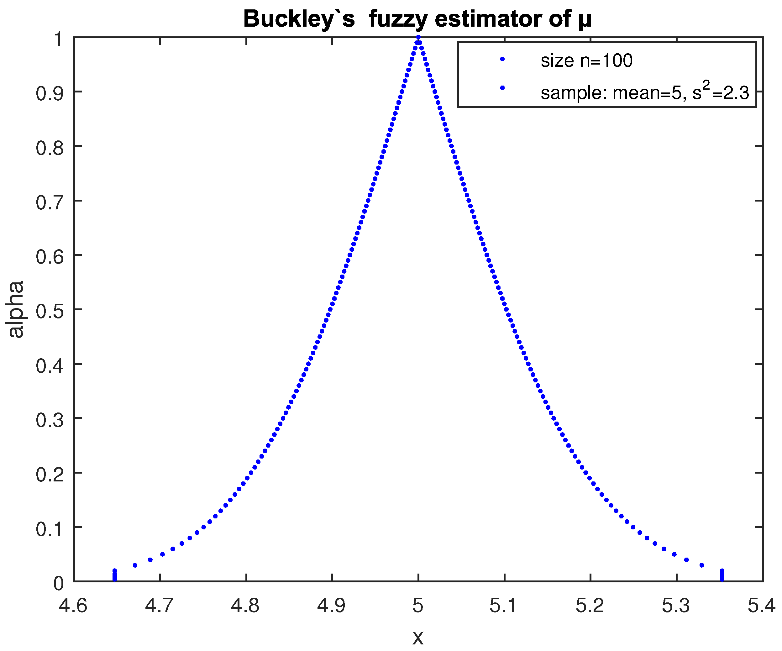
To finish the “bottom” of in order to make it a complete fuzzy number, one needs to drop its graph straight down to complete its cuts (see Figure 1). So, a fuzzy estimator of is produced from a given sample, the possibility distribution of which are the confidence intervals of
The fuzzy estimator produced in this way contains much more information than just a single interval estimate.
For the construction of test statistics used in fuzzy hypothesis testing about an unknown parameter , we use the fuzzy estimator , the -cuts of the possibility distribution of which are the confidence intervals of
since, as proved in [32], this possibility distribution is identical to the one obtained by the maximal specificity probability–possibility transformation. In order to easily handle the possibility representation, especially for further computations, the possibility distribution is restricted to the interval that corresponds to the largest confidence interval for the considered probability distribution (see [32]).
3.1. Estimation of the Mean of a Normal Variable with Known Variance
If the random variable X follows normal distribution with known variance , then the confidence interval of the mean of X derived from a random sample of observations of X of size n and sample mean is [1].
where and , the inverse distribution function of the standard normal distribution. So according to (6), the -cuts of the possibility distribution of the fuzzy estimator of mean are as follows (see [29,30]):
where
Implementing (7), we get the fuzzy estimator of Figure 2.
3.2. Estimation of the Mean of a Random Variable from a Large Sample (with Unknown Variance)
If the random variable X follows any distribution, then, according to the central limit theorem (see [1]), the confidence interval of the mean of X derived from a random sample of observations of X of large size n () with sample mean and variance and is given by (6), substituting with s. So according to (5), the -cuts of the possibility distribution of the fuzzy estimator of the mean are as follows:
where is given by (8).
3.3. Estimation of the Variance of a Normal Variable
If the random variable X follows normal distribution, then the confidence interval of the variance of X derived from a random sample of observations of X of size n and sample variance is as follows [1]:
where ( the inverse distribution function of the distribution)
So according to (5), the -cuts of the possibility distribution of the fuzzy estimator of the variance are as follows:
Therefore, the -cuts of the fuzzy estimator of the standard deviation of X are as follows:
It can be shown that the above fuzzy estimator is biased because its core is not at . A fuzzy estimator of a parameter is defined as biased if its core is not at the crisp point estimator of the parameter.
In [29], an unbiased fuzzy estimator of the variance of a normal random variable is obtained from a sample of size n and variance by putting one above the other for the following confidence intervals:
where
and ( the inverse distribution function of the distribution)
For a value of , the corresponding value of is as follows [29]:
where the probability density function of the distribution. The range of this one to one and onto function is . So, the cuts of the correct unbiased fuzzy estimator are as follows:
where the function and its inverse (it gives as a function of ) are implemented numerically.
In the implementation of of [29], the -cuts defined by (14) (instead of its -cuts of (18)) are used for the construction of and the statistics generated by it.
4. Possibilistic Statistical Tests of Crisp Hypotheses
We denote by 1 the rejection and by 0 the acceptance of a hypothesis for a parameter of the distribution of a random variable X from a sample of n observations of X. Hence, a possibilistic test of a crisp hypothesis with alternative is a decision rule, defined as two functions: , which gives the degree in which the observed value u of the test statistic U belongs to the rejection region (see Section 1) (the possibility of the proposition “u is in the rejection region”), and , which gives the degree in which the observed value u of the test statistic U belongs to the acceptance region (see Section 1) (the possibility of the proposition “u is in the acceptance region”).
Using the fuzzy estimator of (see Section 2) and interval arithmetics, we derive the -cuts of the possibility distribution of the respective fuzzy test statistic . So, the possibilities of rejection or acceptance of are as follows:
(a) For one sided test from the right (alternative hypothesis ), the possibility of rejection of is equal to the Necessity of Strict Dominance index (see [23,36]).
which represents the necessity that the fuzzy set strictly dominates the fuzzy set of the right critical value , the membership function of which is as follows:
where is the critical value of the one sided from the right, defined in (1). So if the core of is at the right of , (19) gives the following:
where is the left part of the possibility distribution and is the ordinate of the point of intersection of with the vertical at .
The possibility of acceptance of is as follows:
which represents the necessity that the fuzzy set strictly dominates the fuzzy set of . So if the core of is at the left of , (22) gives the following:
where is the right part of the possibility distribution and is the ordinate of the point of intersection of with the vertical at .
(b) For , the one sided test from the left (alternative hypothesis ), the possibility of rejection of is equal to the Necessity of Strict Dominance index of to , where the membership function of the critical value is as follows ( the critical value of the one sided from the left defined in (2)):
So if the core of is at the left of , (25) gives the following:
where is the ordinate of the point of intersection of the right part of the possibility distribution of with the vertical at .
The possibility of acceptance of is as follows:
So if the core of is at the right of , (27) gives the following:
where is the ordinate of the point of intersection of the left part of the possibility distribution of with the vertical at .
(c) For the two-sided test (alternative hypothesis ), the possibility of rejection of is equal to the following:
where ( and are the critical values of the two-sided defined in (3)).
So if the core of is at the right of , (33) gives the following:
where and if it is at the left of , it gives the following:
where .
The possibility of acceptance of is as follows:
So if the core of is between and , (34) gives the following:
where and (the ordinates of the point of intersection of the right part of the possibility distribution of with the vertical at and of its left part with the vertical at ).
If the possibility of the rejection or acceptance of is very low (for example lower than ), then we cannot make a decision on rejecting or accepting .
5. Tests on the Mean of a Normal Distribution with Known Variance or of Any Distribution from a Large Sample
We test at the significance level the null hypothesis for the mean of a random variable X, which follows the normal distribution with known variance , using a random sample of observations of X of size n.
In the crisp case, we test , using the statistic (see [1]).
where is the statistic of the sample mean. It is known that under the null hypothesis () Z follows the standard normal distribution , so is rejected from a given sample:
(a) For the one sided test from the right, if
(b) For the one sided test from the left, if ,
(c) For the two sided test, if or , where
the value of the statistic (35) for the given sample,
and the inverse distribution function of the standard normal distribution. Meanwhile, is not rejected if .
In the fuzzy case, the test of is based on the fuzzy statistic
which is generated by substituting in (35) with the fuzzy estimator of the mean value for the given sample, the cuts of the membership function of which are given by (7).
From (38), (7) and interval arithmetics follow that the cuts of the possibility distribution of the fuzzy statistic are as follows:
Hence, the cuts of the possibility distribution of for the given sample are as follows:
where the crisp value of the statistic Z for this sample, which is given by (36).
The membership functions of the critical values and of the one-sided tests are as follows:
and for the two-sided test,
Having the cuts of the possibility distribution of the fuzzy statistic of (39) and the critical values and , we can evaluate the possibility of the rejection or acceptance of from (21), (23), (26), (28) for and (40) for one sided tests or from (31), (32), (34) and (41) for the two-sided test.
If the sample is large and X follows any distribution, then in the crisp case, we test using the statistic
where is the statistic of the sample mean and s, the sample standard deviation [1]. It is known that under the null hypothesis (), Z follows the standard normal distribution according to the central limit theorem [1], so is rejected or not by one sided tests, using (21), (23), (26), (28) for given in (39) for the following sample value:
of the statistic Z or (31), (32), (34) for the two-sided test.
Example 1.
We test the null hypothesis at significance level with alternative (two-sided test) for the mean value μ of the temperature X, using the two large random samples of 50 observations each of the Appendix A (monthly values for selected Greek weather stations) [37].
The mean and the standard deviation of the first sample are and , so in the crisp test, we evaluate the value of the statistic Z for the first sample from (42):
Since
is rejected by this crisp test.
For the second sample the mean and variance are and , so the value of the statistic Z in this case is the following:
Therefore, since the following is true:
is not rejected by the crisp test.
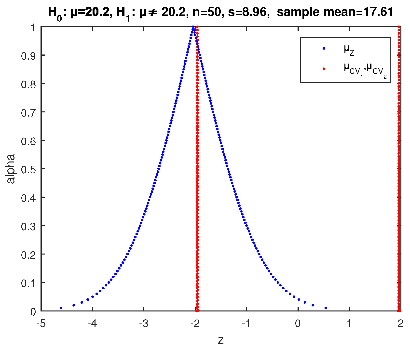
Applying the above described two-sided fuzzy test of , implementing the possibility distribution (39) of for the value of (42) and the critical values (41) for the first sample, we get the results of Figure 4, where the point of intersection of and has . So according to (32), the possibility of rejection of is . Hence, we cannot make a decision on whether to reject or not from this sample.
Implementing (39) and (41) for the second sample, we take Figure 5, where the point of intersection of and has , so according to (34), the possibility of acceptance of is . Therefore, we cannot make a decision on whether to reject or not from this sample.
Example 2.
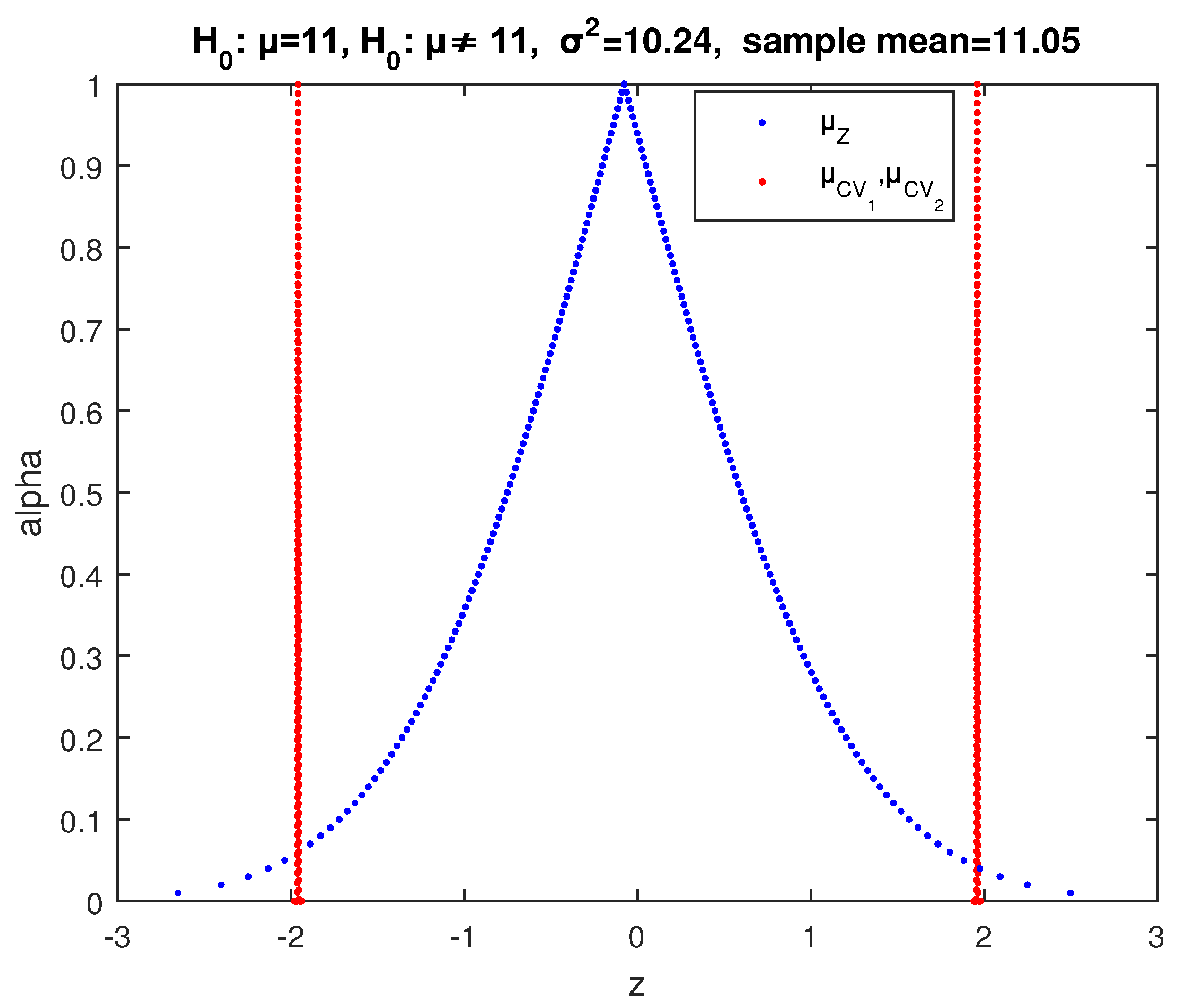
We test at significance level the null hypothesis with alternative (two-sided test) for the mean μ of a random variable X, which follows normal distribution with variance , using a sample of observations with sample mean .
The value of the test statistic (35) is found by (36) to be as follows:
so the crisp p-value of the test is as follows:
Therefore, in this case, the crisp test gives acceptance of with a very high p-value (near to the maximum value, 1).
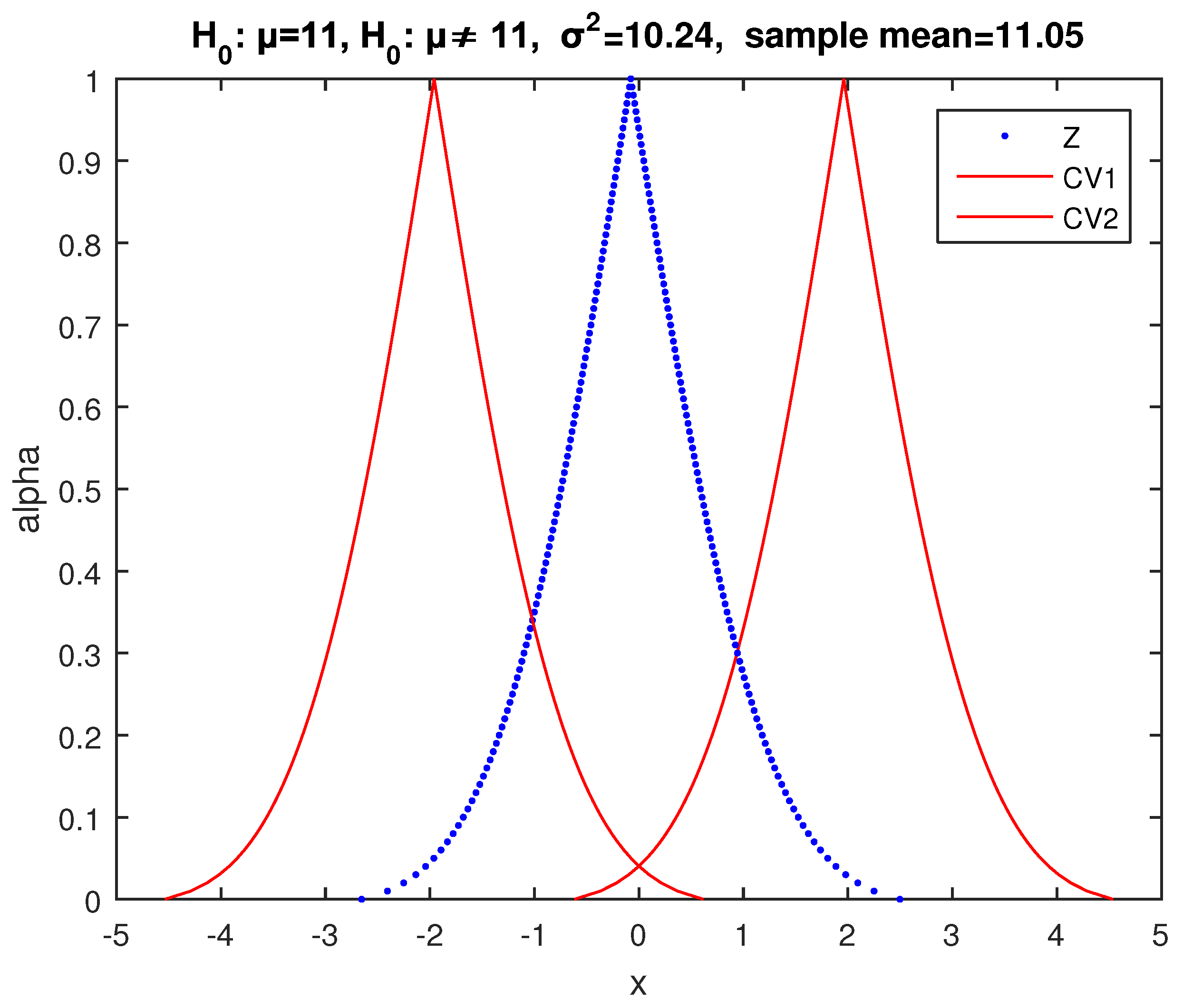
We apply the above two-sided fuzzy test of implementing (39) and (41). So, we obtain the results of Figure 6, where the core of is between the cores of and the point of intersection of , and has and of and has . Hence, according to (34), the possibility of acceptance of is as follows:
so is accepted by this test with possibility .
6. Hypotheses Tests for the Variance of a Normal Distribution
We test at significance level the null hypothesis for the variance of a normal random variable X, using a random sample of observations of X of size n and variance .
In the crisp case, we test , using the test statistic
where is the sample variance, which follows distribution with degrees of freedom under the null hypothesis [1]. is rejected from a given random sample (omitting in the implied degrees of freedom):
(a) For one-sided test from the left (alternative ), if
and is the inverse distribution function of the distribution.
(b) For one-sided test from the right (alternative ), if
(c) For two-sided test (alternative ), if
where
and
the crisp value of the statistic (43). Otherwise, is not rejected.
In the fuzzy case for the test of , we use the fuzzy statistic generated by substituting in (43) with a fuzzy estimator of the following variance:
Using the cuts of the unbiased fuzzy estimator given in (14) and interval arithmetics, we obtain from (48) the cuts of the possibility distribution of the following test statistic:
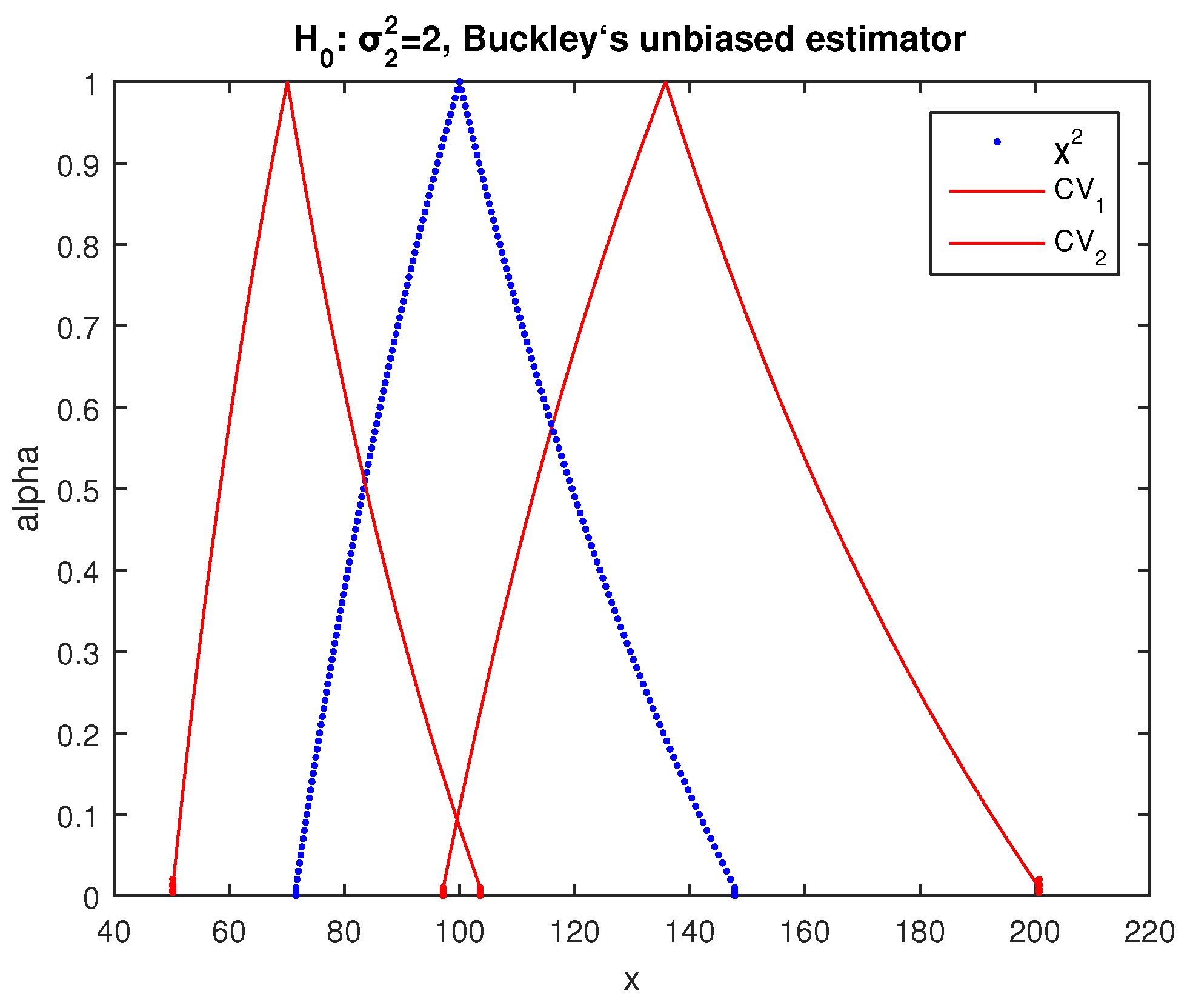
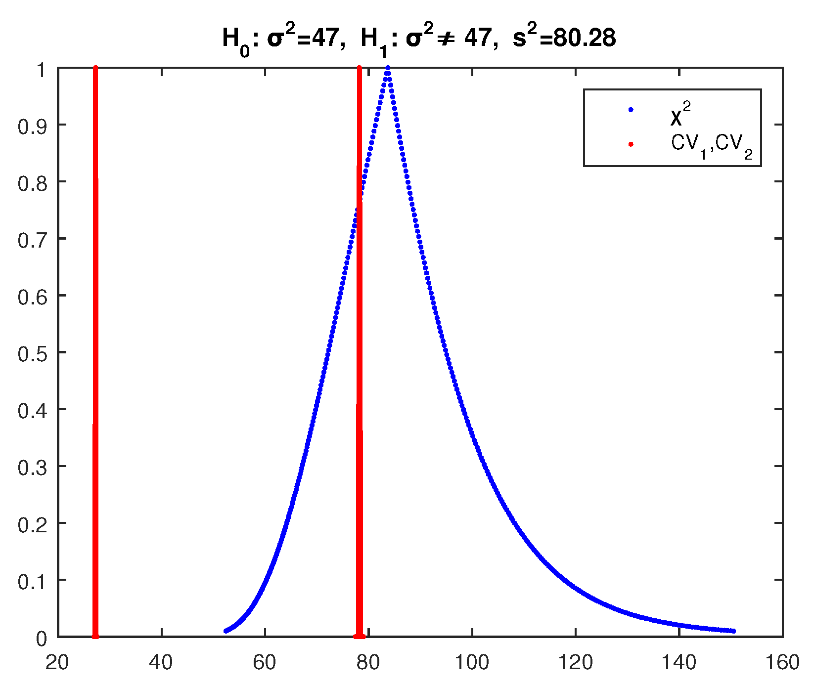
As illustrated in Figure 8 and Figure 9, the shape of this test statistic is significantly different than the shape of the respective test statistic produced by the implementation of used in [29], which is as expected since the shape of the two implementations (14) and (18) of are different.
The membership functions of the critical values and of one-sided tests are as follows:
and for the two-sided test
where the inverse distribution function of the distribution with degrees of freedom.
Having the cuts of the possibility distribution of the fuzzy statistic and the critical values and , we can evaluate the possibility of rejection or acceptance of from (21), (23), (26), (28) for and (50) for one sided tests or from (31), (32), (34) and (51) for two sided test.
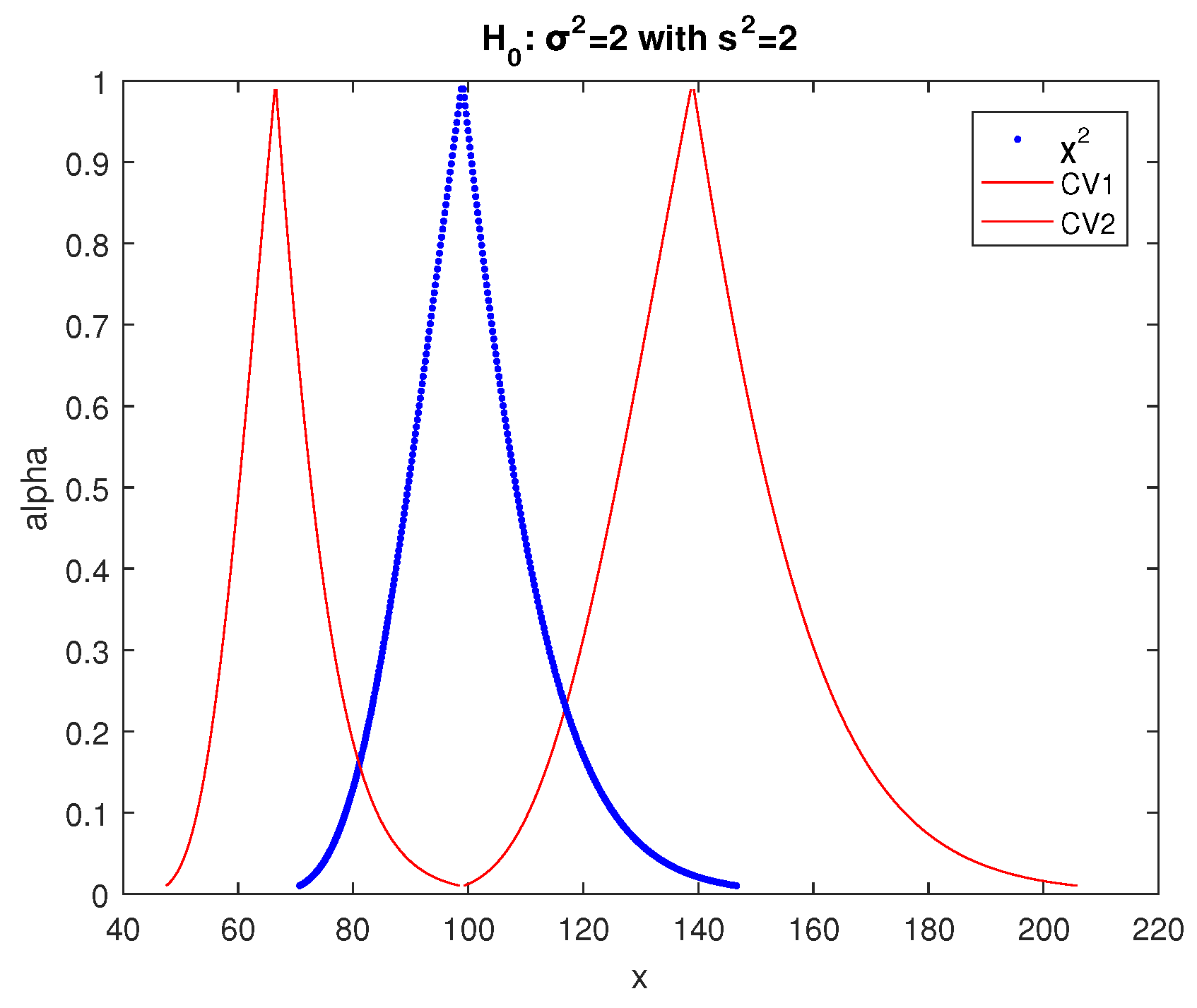
Example 3.
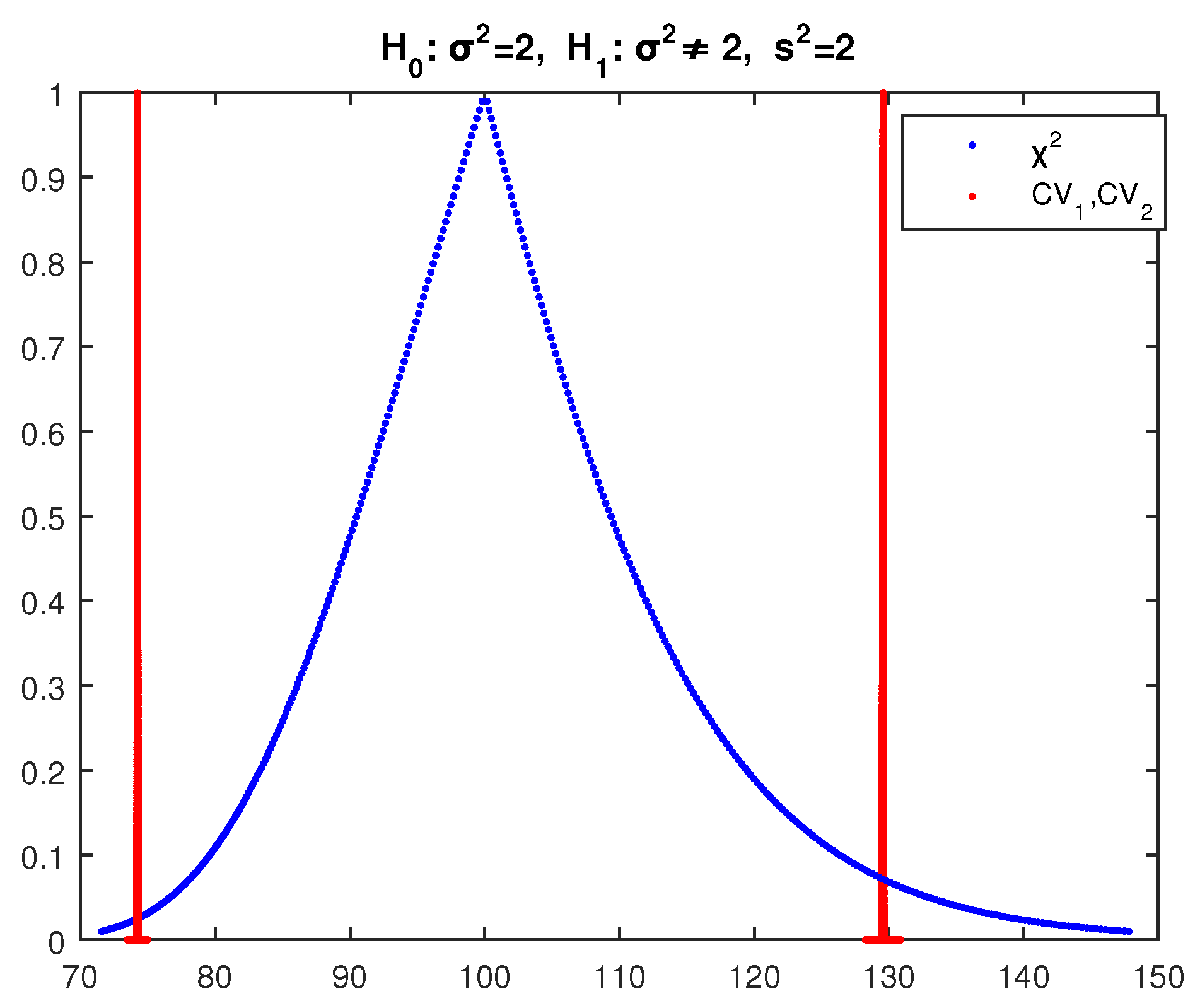
We test at significance level the null hypothesis with alternative for the variance of a normal random variable, using a random sample of 101 observations with sample variance .
The crisp test in this case gives acceptance of with the largest possible difference between the test statistic and the critical values since the p-value is 1 (the test statistic is exactly in the middle of the no-rejection region), so it is the best case for the acceptance of .
Applying the above fuzzy test, we get the results of Figure 8, where the core of is between the cores of and and the point of intersection of , and has and of and , , so according to (34) the possibility of acceptance of is as follows:
The respective fuzzy test of of [29] gives the results of Figure 9, where the possibility of acceptance of is as follows:
and the test of of [30] gives the results of Figure 10, where the possibility of acceptance of is as follows:
The results of the fuzzy hypothesis tests proposed in this paper are in much better agreement with the results of the respective crisp tests than the results of the respective tests of [29]. This happens because of the following:
- (1)
- The former are based on the correct implementation of , according to the theory, whereas the latter contain the error of using -cuts instead of -cuts.
- (2)
- The tests of [29] use fuzzy critical values, which are created using probabilistic concepts.
The above are illustrated by the characteristic case of the hypothesis test of Example 3 in which the crisp value of the test statistic is exactly in the middle of the acceptance region (p-value), which is the best case of acceptance. As shown in this example, the test, which uses the implementation of of [29], gives a significantly lower possibility of acceptance of () than the test which uses our implementation of (). So, the latter is in much better agreement with the crisp statistical tests than the former.
The possibilistic tests developed in this paper are in better agreement with the results of the respective crisp tests than the results of the tests of [30], which also use the same fuzzy critical values as [29]. This is illustrated in Examples 2 and 3 in which the crisp value of the test statistic is exactly in the middle of the acceptance region. As shown in these examples, the tests of [30] give a significantly lower degree of acceptance of ( for Example 2 and for Example 3) than the respective tests of this paper ( for both examples). So, the latter are in better agreement with the crisp statistical test than the former. This happens in all relevant examples (statistic in the middle of the acceptance region).
Example 4.
We test the null hypothesis at significance level with alternative (two-sided test) for the variance of the temperature X, using the two large random samples of 50 observations each of the Appendix A (monthly values for selected Greek weather stations) [37].
The crisp value of the test statistic (43) for the first sample is found by (47) to be as follows (the sample variance is ):
The critical values of this crisp test are (, the inverse distribution function of the distribution).
So since , is rejected by the crisp test for this sample.
For the second sample (variance ), the value of the test statistic (43) is found by (47) to be as follows:
So since is not rejected by the crisp test for this sample.
Applying the above fuzzy test for the first sample, we get the results of Figure 11, where the core of is at the right of the core of and their point of intersection has . So according to (31), the possibility of rejection of is as follows:
For the second sample, we get the results of Figure 12, where the core of is between the cores of and and the point of intersection of and has and of and , . So according to (34), the possibility of acceptance of is as follows:
Therefore, we cannot make a decision on accepting from this test.
7. Hypothesis Tests for the Mean of a Normal Random Variable with Unknown Variance
We test at significance level the null hypothesis for the mean value of a random variable X, which follows normal distribution with unknown variance, using a random sample of observations of X of size n with sample mean and variance and .
In this case, the test statistic is
where and S are the statistics of the sample mean and the standard deviation.
It is known [1] that under the null hypothesis (), T follows t distribution with degrees of freedom. So in the crisp case, is rejected from a given random sample:
(a) For the one sided test from the right (alternative ), if , where
the value of the statistic (52),
the critical value of the test and is the inverse distribution function of the t distribution with degrees of freedom.
(b) For the one sided test from the left (alternative ), if .
(c) For the two-sided test ( alternative ), if or while, if , then is not rejected.
In the fuzzy case for the test of we use the following fuzzy statistic:
which is generated by substituting and S in (52) with the fuzzy estimators and of the mean and standard deviation. The cuts of are given by (13) and (as described in [29,30]) the cuts of the possibility distribution of are as follows:
From (53), (55), (56), (13) and fuzzy number arithmetics follows that the cuts of the possibility distribution of the fuzzy statistic are as follows:
where .
The membership functions of the critical values and of the one-sided tests are as follows:
and for the two-sided test,
where is the inverse distribution function of the t distribution with degrees of freedom.
Having the cuts (57) of the possibility distribution of the fuzzy statistic T and the critical values and , we can evaluate the possibility of rejection or acceptance of from (21), (23), (26), (28) for and (58) for one-sided tests or from (31), (32), (34) and (59) for the two-sided test.
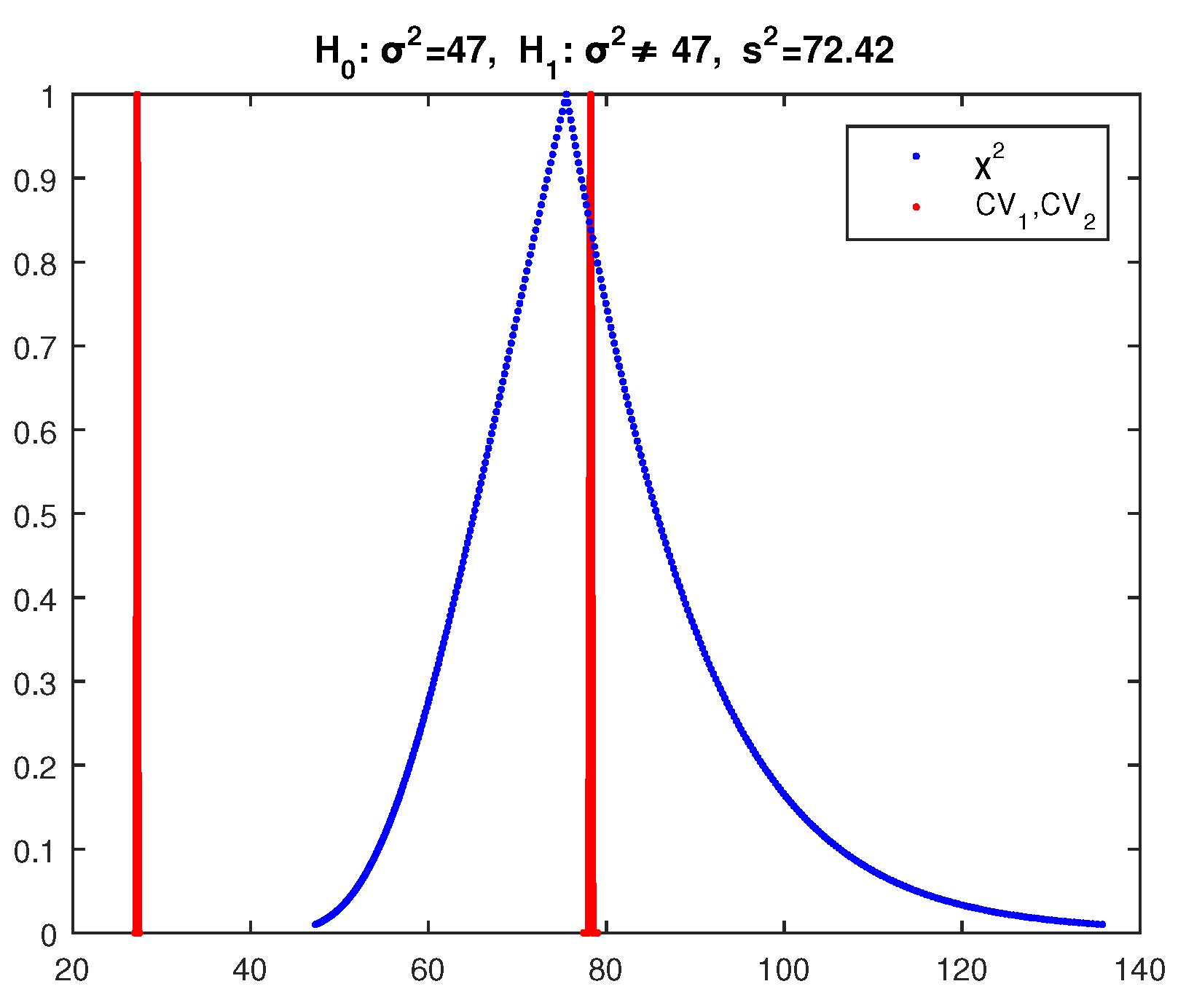
Example 5.
We test the null hypothesis at significance level with alternative (two sided test) for the mean μ of a normal random variable X, using a sample of observations with sample mean and variance and .
In the crisp case, the value of the statistic (52) is evaluated by (53)
so the value is , which is much higher than the significance level . Hence, is accepted by the crisp test with high p-value (the test statistic is almost at the center of the acceptance region).
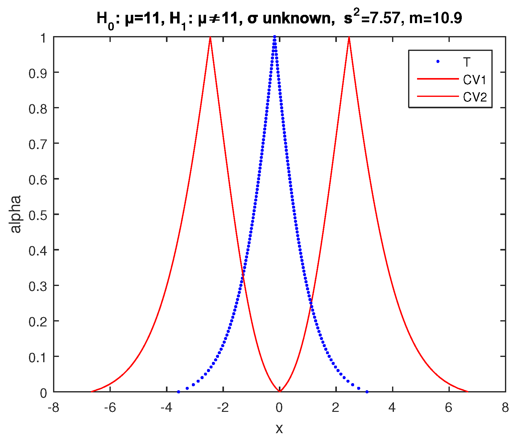
We apply the above two-sided fuzzy test of , implementing (57) and (59). So, we obtain the results of Figure 13, where the core of is between the cores of and and the points of intersection of and and of and have and . Hence, according to (34), the possibility of acceptance of is
so is accepted by this test with possibility .
Applying the respective test of [29,30], we get the results of Figure 14, where we see that the possibility of acceptance of is as follows:
Example 6.
We test the null hypothesis at significance level with alternative (two sided test) for the mean μ of a normal random variable X, using a sample of observations with sample mean and variance and .
In the crisp case, the value of the statistic (52) is evaluated by (53)
so the value is , which is almost zero. Hence, is rejected by the crisp test.
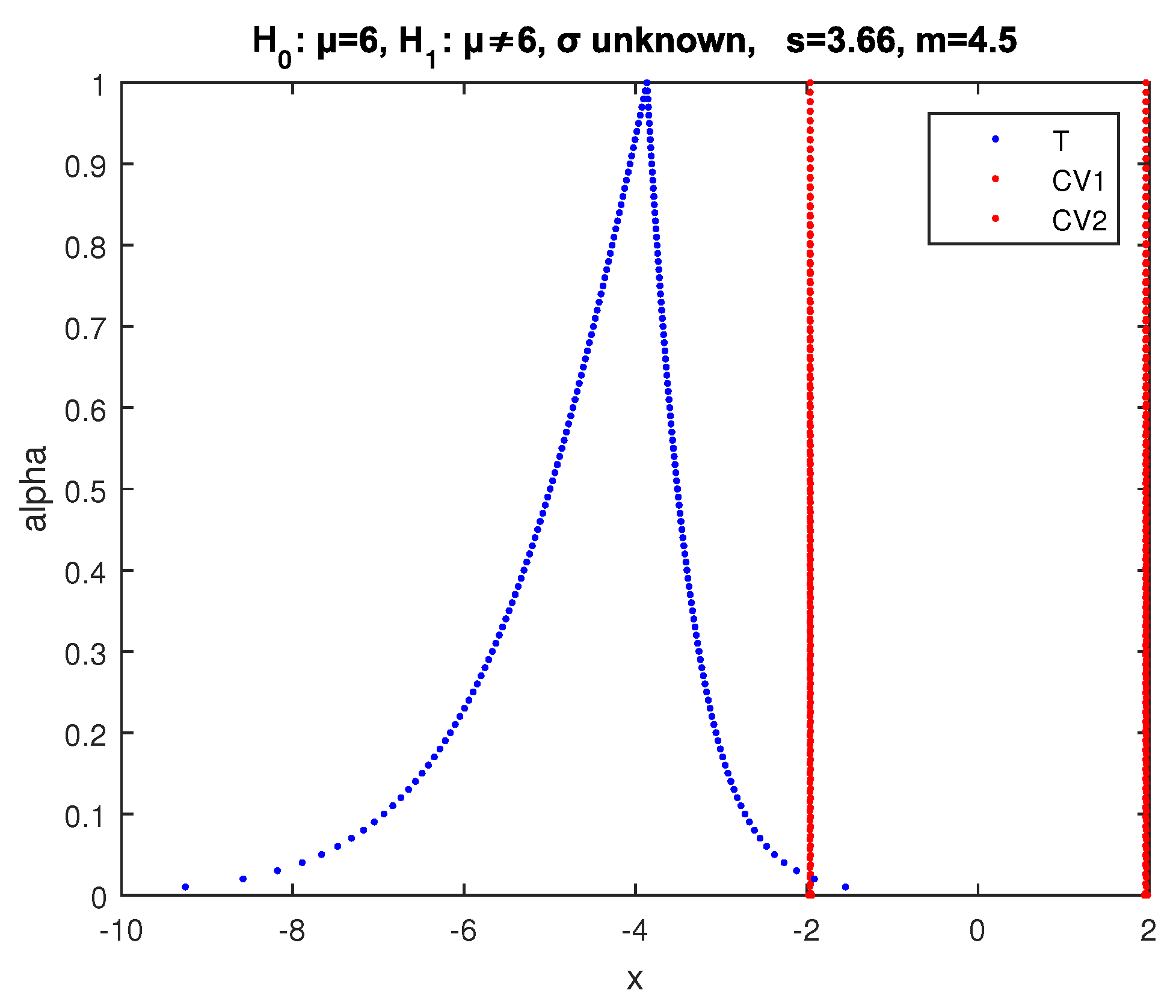
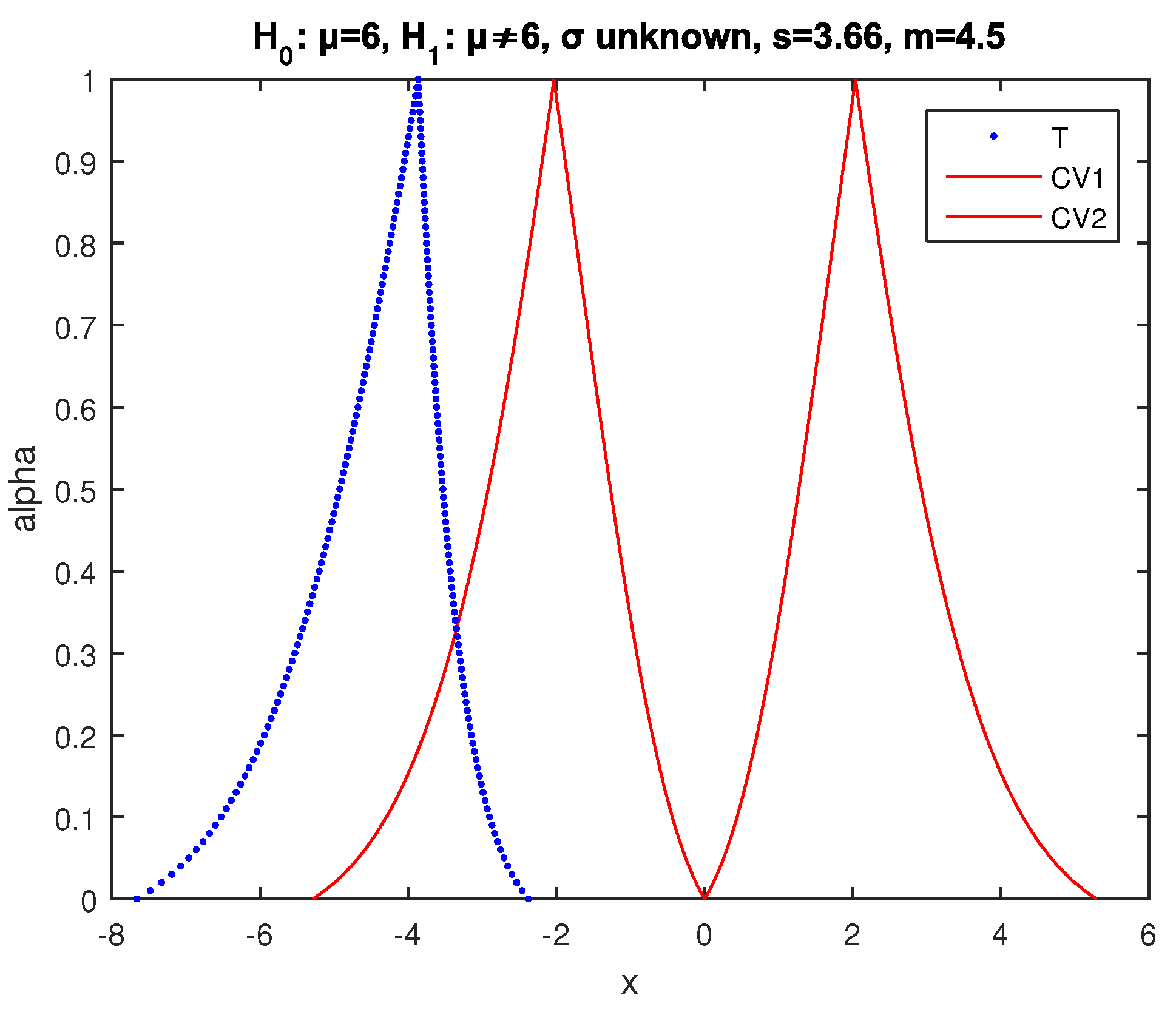
We apply the above test implementing (57) and (59). So, we take the results of Figure 15, where the core of is at the left of the core of and the point of intersection of and has . Hence, according to (32), the possibility of rejection of is .
Applying the respective test of [30], we get the results of Figure 16, where we see that the possibility of acceptance of is as follows:
A similar result with even lower possibility of acceptance is obtained by the respective test of [29].
8. Conclusions
If the value of the test statistic of a hypothesis is close to a critical value of the test, then the crisp hypothesis test is unstable since a very small change in the sample may lead from rejection to no rejection of or vice-versa, as shown in Examples 1 and 4. Our possibilistic approach, which uses fuzzy estimators for the construction of the test statistic and a possibility of rejection or acceptance of the null hypothesis , gives better results than the crisp test since it gives us the possibility of rejection or acceptance of , as shown in Examples 1 and 4, where we get a very low possibility of rejection or acceptance of the null hypothesis, which means “no decision”.
We can also conclude the following:
- (1)
- The use of the fuzzy critical values of [29,30] in hypothesis tests leads to wrong results, since they are not in good agreement with the crisp tests, which have been known for nearly one hundred years (Examples 2, 3 and 5). Meanwhile, the possibilistic fuzzy hypothesis tests developed in this paper give results which are in much better agreement with the crisp tests.
- (2)
- The use of the implementation of of [29] in the hypothesis tests leads, also, to wrong results since they are not in good agreement with the crisp tests (Example 3). Meanwhile, the fuzzy hypothesis tests, which are based on test statistics produced by the correct implementation of (taking into consideration the relation between the significance level a and the parameter ), give results which are in better agreement with the crisp tests.
We believe that with the help of all the above, new horizons can be opened in the fuzzy hypothesis testing of several topics, such as the following:
- (a)
- (b)
- (c)
- The regression coefficient and the predicted value of Y for a given in a linear regression model , using fuzzy test statistics constructed by the fuzzy estimators and produced by the known classical statistics confidence intervals, of ( and the sample regression coefficient and its standard deviation) and of ( and the predicted value of Y for from the given sample and its standard deviation).
Author Contributions
Data curation, N.M.; Formal analysis, B.P. All authors have read and agreed to the published version of the manuscript.
Funding
This research received no external funding.
Institutional Review Board Statement
Not applicable.
Informed Consent Statement
Not applicable.
Acknowledgments
We would like to thank the referees for their valuable remarks and suggestions.
Conflicts of Interest
The authors declare no conflict of interest.
Appendix A
Samples of temperature taken from Hellenic national meteorological service [37].
| Sample 1 |
| Sample 2 |
References
- Hogg, R.V.; Tanis, E.A. Probability and Statistical Inference, 6th ed.; Prentice Hall: Upper Saddle River, NJ, USA, 2001. [Google Scholar]
- Zadeh, L.A. Fuzzy sets. Inf. Control 1965, 8, 338–353. [Google Scholar] [CrossRef] [Green Version]
- Taheri, S.M. Trends in fuzzy statistics. Aust. J. Stat. 2003, 32, 239–257. [Google Scholar] [CrossRef]
- Tanaka, H.; Okuda, T.; Asai, K. Fuzzy information and decision in a statistical model. In Advances in Fuzzy Set Theory and Applications; Gupta, M.M., Ragade, R.K., Yager R., R., Eds.; North-Holland: Amsterdam, The Netherlands, 1979; pp. 303–320. [Google Scholar]
- Casals, M.R.; Gil, M.A.; Gil, P. On the use of Zadeh’s probabilistic definition for testing statistical hypotheses from fuzzy information. Fuzzy Sets Syst. 1986, 20, 175–190. [Google Scholar] [CrossRef]
- Casals, M.R. Bayesian testing of fuzzy parametric hypotheses from fuzzy information. Oper. Res. 1993, 27, 189–199. [Google Scholar] [CrossRef] [Green Version]
- Watanabe, N.; Imaizumi, T. A fuzzy statistical test of fuzzy hypotheses. Fuzzy Sets Syst. 1993, 53, 167–178. [Google Scholar] [CrossRef]
- Arnold, B.F. An approach to fuzzy hypothesis testing. Metrika 1996, 44, 119–126. [Google Scholar] [CrossRef]
- Arnold, B.F. Testing fuzzy hypotheses with crisp data. Fuzzy Sets Syst. 1998, 94, 323–333. [Google Scholar] [CrossRef]
- Taheri, S.M.; Behboodian, J. Neyman-Pearson Lemma for fuzzy hypotheses testing. Metrika 1999, 49, 3–17. [Google Scholar] [CrossRef]
- Taheri, S.M.; Behboodian, J. ABayesian approach to fuzzy hypotheses testing. Fuzzy Sets Syst. 2001, 123, 39–48. [Google Scholar] [CrossRef]
- Chachi, J.; Taheri, S.M. Optimal statistical tests based on fuzzy random variables. Iran. J. Fuzzy Syst. 2018, 15, 27–45. [Google Scholar]
- Akbari, M.G.; Hesamian, G. Testing statistical hypotheses for intuitionistic fuzzy data. Soft Comput. 2019, 23, 10385–10392. [Google Scholar] [CrossRef]
- Arefi, M. Testing statistical hypotheses under fuzzy data and based on a new signed distance. Iran. J. Fuzzy Syst. 2018, 15, 153–176. [Google Scholar]
- Hung, J.-L.; Chen, C.-C.; Lai, C.-M. Possibility Measure of Accepting Statistical Hypothesis. Mathematics 2020, 8, 551. [Google Scholar] [CrossRef] [Green Version]
- Chukhrova, N.; Johannssen, A. Fuzzy hypothesis testing for a population proportion based on set-valued information. Fuzzy Sets Syst. 2020, 387, 127–157. [Google Scholar] [CrossRef]
- Chukhrova, N.; Johannssen, A. Randomized versus non-randomized hypergeometric hypothesis testing with crisp and fuzzy hypotheses. Stat. Pap. 2018, 61, 1–37. [Google Scholar] [CrossRef]
- Filzmoser, P.; Viertl, R. Testing hypotheses with fuzzy data: The fuzzy p-value. Metrika 2004, 59, 21–29. [Google Scholar] [CrossRef]
- Parchami, A.; Taheri, S.M.; Mashinchi, M. Fuzzy p-value in testing fuzzy hypotheses with crisp data. Stat Pap. 2010, 51, 209. [Google Scholar] [CrossRef]
- Mylonas, N.; Papadopoulos, B. Fuzzy p-value of Hypotheses Tests with Crisp Data Using Non-Asymptotic Fuzzy Estimators. J. Stoch. Anal. 2021, 2, 1. [Google Scholar] [CrossRef]
- Couso, I.; Sanchez, L. Mark-recapture techniques in statistical tests for imprecise data. Internat. J. Approx. Reason. 2011, 52, 240–260. [Google Scholar] [CrossRef] [Green Version]
- Grzegorzewski, P.; Hryniewicz, O. Soft methods in hypotheses testing. In Soft Computing for Risk Evaluation and Management: Applications in Technology, Environment and Finance, in Studies in Fuzziness and Soft Computing; Ruan, D., Kacprzyk, J., Fedrizzi, M., Eds.; Physica-Verlag: Heidelberg, Germany, 2001; Volume 76, pp. 55–72. [Google Scholar]
- Hryniewicz, O. Possibilistic decisions and fuzzy statistical tests. Fuzzy Sets Syst. 2006, 157, 2665–2673. [Google Scholar] [CrossRef]
- Hryniewicz, O. Statistical properties of the fuzzy p-value. Internat. J. Approx. Reason. 2018, 93, 544–560. [Google Scholar] [CrossRef]
- Berkachy, R.; Donze, L. Testing hypotheses by fuzzy methods: A comparison with the classical approach. In Applying Fuzzy Logic for the Digital Economy and Society, in Fuzzy Management Methods; Meier, A., Portmann, E., Teran, L., Eds.; Springer: Cham, Switzerland, 2019; pp. 1–22. [Google Scholar]
- Parchami, A. Fuzzy decision making in testing hypotheses: An introduction to the packages FPV and fuzzy.p.value with practical examples. Iran. J. Fuzzy Syst. 2020, 17, 67–77. [Google Scholar]
- Chukhrova, N.; Johannssen, A. Fuzzy hypothesis testing: Systematic review and bibliography. Appl. Soft Comput. 2021, 106, 107331. [Google Scholar] [CrossRef]
- Buckley, J.J. Fuzzy statistics: Hypotheses testing. Soft Comput. 2005, 9, 512–518. [Google Scholar] [CrossRef]
- Buckley, J.J. Fuzzy Statistics; Springer: Berlin/Heidelberg, Germany, 2004. [Google Scholar]
- Mylonas, N.; Papadopoulos, B. Fuzzy hypotheses tests for crisp data using non-asymptotic fuzzy estimators and a degree of rejection or acceptance. Evol. Syst. 2021, 1–18. [Google Scholar] [CrossRef]
- Sfiris, D.; Papadopoulos, B. Non-asymptotic fuzzy estimators based on confidence intervals. Inf. Sci. 2014, 279, 446–459. [Google Scholar] [CrossRef]
- Dubois, D.; Foulloy, L.; Mauris, G.; Prade, H. Probability-possibility transformations, triangular fuzzy-sets and probabilistic inequalities. Reliab. Comput. 2004, 10, 273–297. [Google Scholar] [CrossRef]
- Kaya, I.; Kahraman, C. A new perspective on fuzzy process capability indices: Robustness. Expert Syst. Appl. 2010, 37, 4593–4600. [Google Scholar] [CrossRef]
- Kaya, I.; Kahraman, C. Fuzzy Process Capability Analysis and Applications. In Production Engineering and Management under Fuzziness, Studies in Fuzziness and Soft Computing; Kahraman, C., Yavuz, M., Eds.; Springer: Berlin/Heidelberg, Germany, 2010; Volume 252, pp. 483–513. [Google Scholar]
- Senvar, O.; Tozan, H. Process Capability and Six Sigma Methodology Including Fuzzy and Lean Approaches. In Products and Services from R and D to Final Solutions; Fuerstner, I., Ed.; IntechOpen, 2010; Available online: https://www.intechopen.com/books/products-and-services–from-r-d-to-final-solutions/process-capability-and-six-sigma-methodology-including-fuzzy-and-lean-approaches (accessed on 1 January 2020). [CrossRef] [Green Version]
- Dubois, D.; Prade, H. Ranking of fuzzy numbers in the setting of possibility theory. Inf. Sci. 1983, 30, 183–224. [Google Scholar] [CrossRef]
- Hellenic National Meteorological Service. Available online: http://www.hnms.gr/emy/el/climatology/climatologymonth (accessed on 1 January 2020).
Figure 1.
Buckley’s fuzzy estimator of the mean of a random variable X, which follows normal distribution with variance , derived from a sample of observations with sample mean .
Figure 1.
Buckley’s fuzzy estimator of the mean of a random variable X, which follows normal distribution with variance , derived from a sample of observations with sample mean .

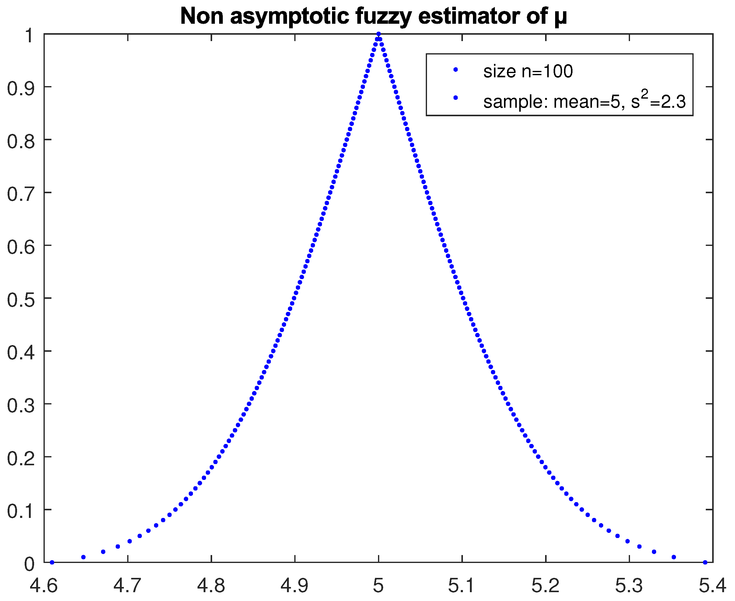
Figure 2.
The possibility distribution of the fuzzy estimator of the mean of a random variable X, which follows normal distribution with variance derived from a sample of observations with sample mean .
Figure 2.
The possibility distribution of the fuzzy estimator of the mean of a random variable X, which follows normal distribution with variance derived from a sample of observations with sample mean .

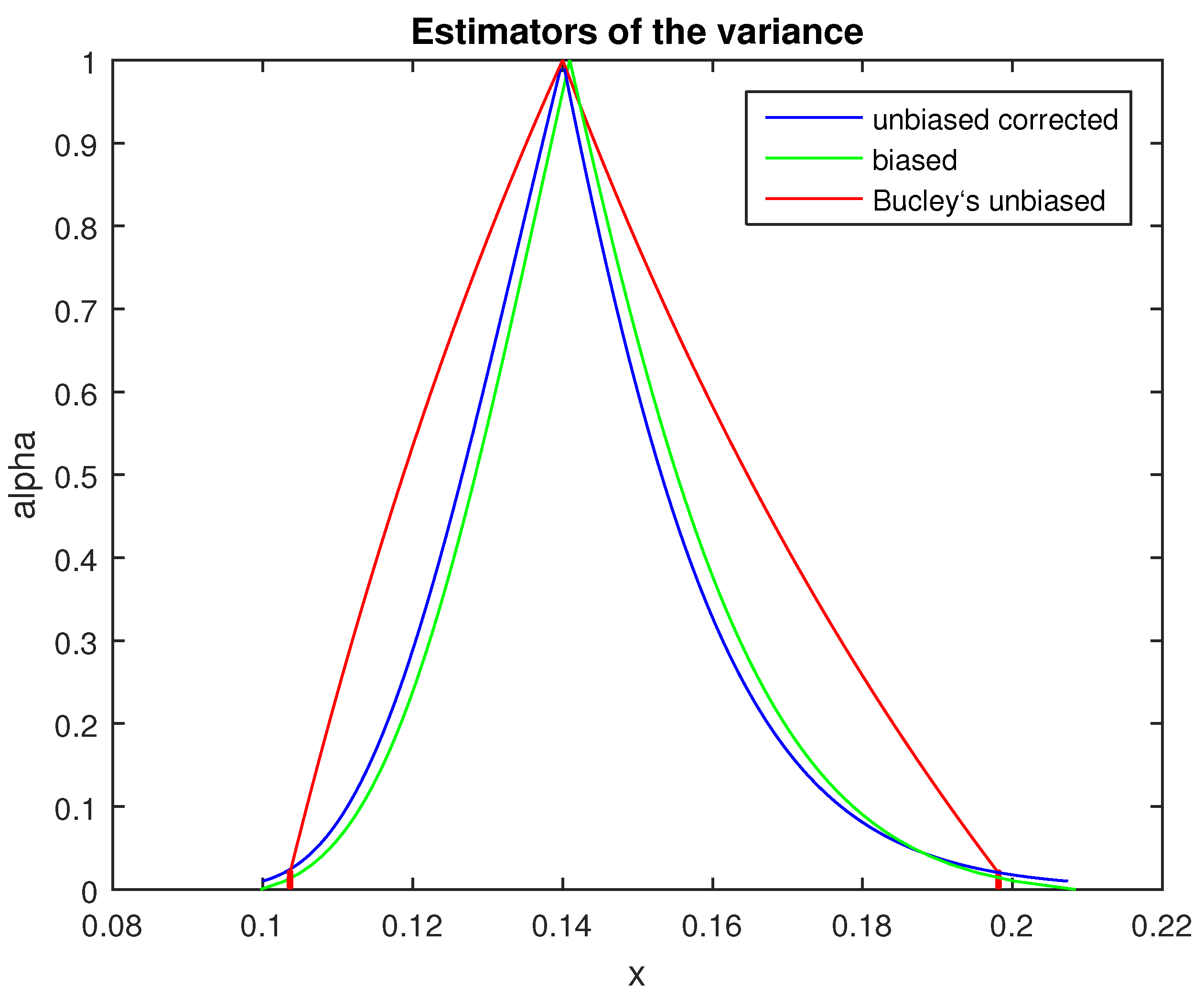
Figure 3.
Non-asymptotic fuzzy estimators of the variance : correct unbiased (blue line), biased (green line), unbiased used in [29] (red line).
Figure 3.
Non-asymptotic fuzzy estimators of the variance : correct unbiased (blue line), biased (green line), unbiased used in [29] (red line).

Figure 4.
The possibility distribution of the fuzzy statistic Z for the test of Example 1 from a sample with .
Figure 4.
The possibility distribution of the fuzzy statistic Z for the test of Example 1 from a sample with .

Figure 5.
The possibility distribution of the fuzzy statistic Z for the test of Example 1 from a sample with .
Figure 5.
The possibility distribution of the fuzzy statistic Z for the test of Example 1 from a sample with .

Figure 6.
The possibility distribution of the fuzzy statistic for the two-sided test of Example 2.

Figure 7.
Fuzzy statistic and critical values for the respective test of Example 2 in [30].
Figure 7.
Fuzzy statistic and critical values for the respective test of Example 2 in [30].

Figure 8.
The possibility distribution of the fuzzy statistic for the test of of Example 3.

Figure 9.
The possibility distribution of the fuzzy statistic and the fuzzy critical values for the respective test of of Example 3 in [29].
Figure 9.
The possibility distribution of the fuzzy statistic and the fuzzy critical values for the respective test of of Example 3 in [29].

Figure 10.
The possibility distribution of the fuzzy statistic and critical values for the respective test of of Example 3 in [30].
Figure 10.
The possibility distribution of the fuzzy statistic and critical values for the respective test of of Example 3 in [30].

Figure 11.
The fuzzy statistic for the test of Example 4 for a sample with variance .

Figure 12.
The possibility distribution of the fuzzy statistic for the test of Example 4 for a sample with variance .
Figure 12.
The possibility distribution of the fuzzy statistic for the test of Example 4 for a sample with variance .

Figure 13.
The possibility distribution of the fuzzy statistic for the test of of Example 5.

Figure 14.
The possibility distribution of the fuzzy statistic and the fuzzy critical values for the respective test of [15] of of Example 5.
Figure 14.
The possibility distribution of the fuzzy statistic and the fuzzy critical values for the respective test of [15] of of Example 5.

Figure 15.
The fuzzy statistic for the test of Example 6.

Figure 16.
The fuzzy statistic and the fuzzy critical values for the test of of [30] for Example 6.
Figure 16.
The fuzzy statistic and the fuzzy critical values for the test of of [30] for Example 6.

Publisher’s Note: MDPI stays neutral with regard to jurisdictional claims in published maps and institutional affiliations. |
© 2021 by the authors. Licensee MDPI, Basel, Switzerland. This article is an open access article distributed under the terms and conditions of the Creative Commons Attribution (CC BY) license (https://creativecommons.org/licenses/by/4.0/).
Share and Cite
MDPI and ACS Style
Mylonas, N.; Papadopoulos, B. Unbiased Fuzzy Estimators in Fuzzy Hypothesis Testing. Algorithms 2021, 14, 185. https://0-doi-org.brum.beds.ac.uk/10.3390/a14060185
AMA Style
Mylonas N, Papadopoulos B. Unbiased Fuzzy Estimators in Fuzzy Hypothesis Testing. Algorithms. 2021; 14(6):185. https://0-doi-org.brum.beds.ac.uk/10.3390/a14060185
Chicago/Turabian StyleMylonas, Nikos, and Basil Papadopoulos. 2021. "Unbiased Fuzzy Estimators in Fuzzy Hypothesis Testing" Algorithms 14, no. 6: 185. https://0-doi-org.brum.beds.ac.uk/10.3390/a14060185
Note that from the first issue of 2016, this journal uses article numbers instead of page numbers. See further details here.