Dynamical Recovery of Complex Networks under a Localised Attack

Abstract

In real systems, some damaged nodes can spontaneously become active again when recovered from themselves or their active neighbours. However, the spontaneous dynamical recovery of complex networks that suffer a local failure has not yet been taken into consideration. To model this recovery process, we develop a framework to study the resilience behaviours of the network under a localised attack (LA). Since the nodes’ state within the network affects the subsequent dynamic evolution, we study the dynamic behaviours of local failure propagation and node recoveries based on this memory characteristic. It can be found that the fraction of active nodes switches back and forth between high network activity and low network activity, which leads to the spontaneous emergence of phase-flipping phenomena. These behaviours can be found in a random regular network, Erdős-Rényi network and Scale-free network, which shows that these three types of networks have the same or different resilience behaviours under an LA and random attack. These results will be helpful for studying the spontaneous recovery real systems under an LA. Our work provides insight into understanding the recovery process and a protection strategy of various complex systems from the perspective of damaged memory.

1. Introduction

Network science has attracted a lot of attention, and it can map the actual system into a network by treating individuals/entities as nodes and the relationship between individuals as edges [1,2,3]. There is much interest in the question of how to keep the resilience of a system after node or link failures. Previous studies mainly focused on the network structures [3,4,5,6,7], network dynamics [8,9,10,11], and failure mechanisms [12,13,14,15]. Most research on the network assumes that the network is static, while many real systems dynamically evolve. For example, traffic networks with flow changes over time [16], while friendship networks decreased in size with time increasing [17]. For some systems in real-world scenarios, after the collapse, they can spontaneously recover. For example, the transportation network returned to normal after a period of congestion. Additionally, the financial network may recover after most of its components fail from a financial crisis. To model these actual phenomena, Majdandzic et al. [12] developed a framework for understanding dynamic networks based on the node recovery process and found that they can lead to the spontaneous emergence of macroscopic phase-flipping phenomena. Based on this, the model is developed for interacting dynamical networks and shows a very rich phase diagram [14]. After that, the research on recovery networks became an important research topic and has been paid extensive close attention [18,19,20]. For example, Shang proposed the recovery strategy for complex networks under random failures by considering that a fraction of the failed nodes are localised and recovered [21].

However, most researches did not consider the dynamical recovery impact of different failure mechanisms and only studied the network under random failures. In real life, some natural disasters, such as earthquakes, floods, or military attacks on infrastructure networks, often spread from one node to the surroundings in turn [22]. This failure mechanism is named a localised attack (LA) [22,23]. The main difference between an LA and random failure (RA) is that the former is only limited to a local area, while the latter is distributed throughout the whole network. This localised attack on some networks is more destructive than random failure [24,25] because a cluster of nodes failing can trigger an avalanche. Previous studies mainly focused on static networks and did not consider dynamic networks under such failure. However, in real scenarios, such transient dynamics, such as failure propagation, and the recovery process take place by turn after suffering initial failure. Therefore, it is interesting and of practical application to study how to enhance the resilience of dynamic networks against localised attacks based on dynamical recovery.

In this paper, the recovery model is based on three fundamental assumptions: (i) internal failure is independent of the neighbourhood, (ii) external failure is induced by failed neighbouring nodes if their number exceeds a threshold, and (iii) the implementation of spontaneous recovery after a period of time. Here, we mainly focus on the resilience behaviours through the above local failure propagation and recovery strategy.

2. Model and Results

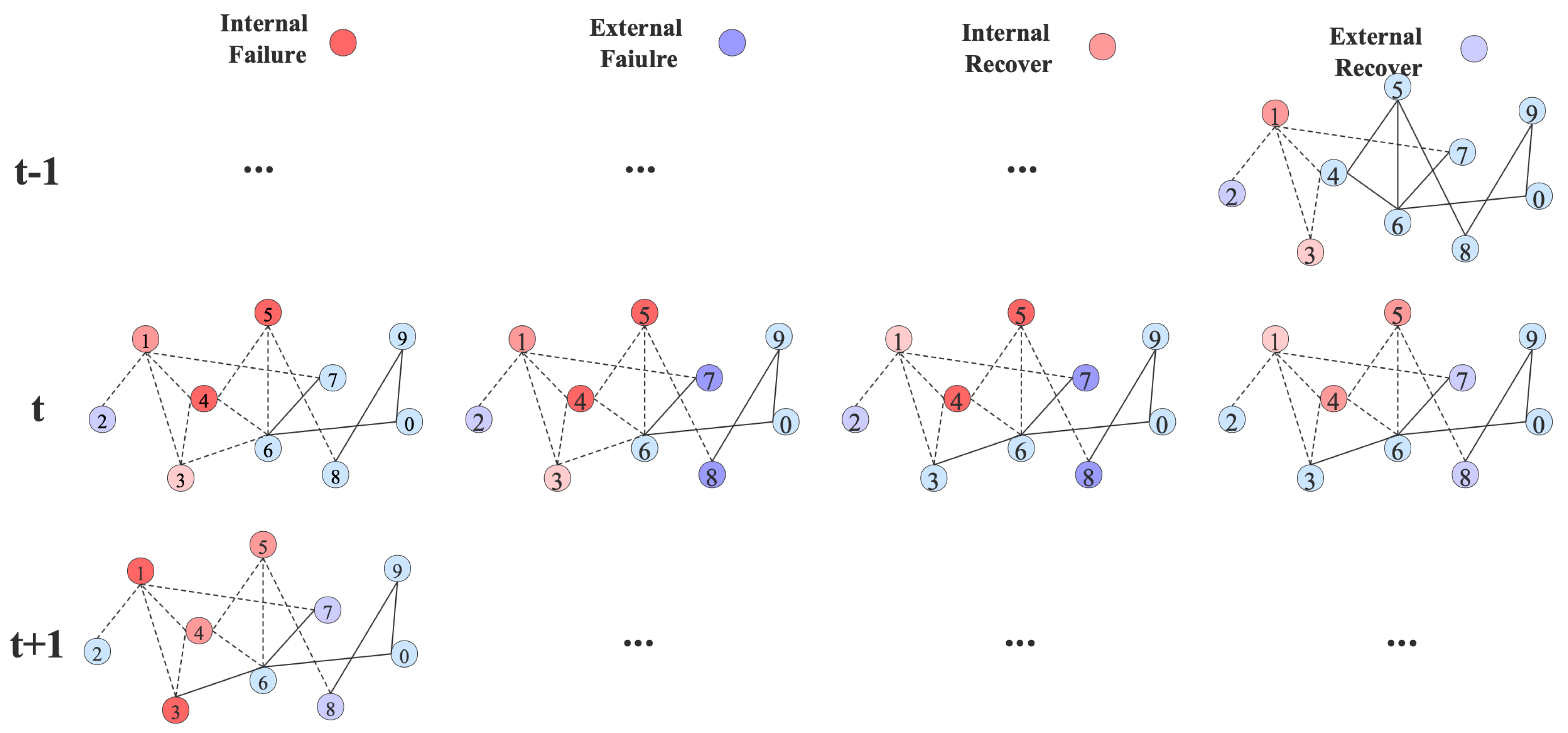
Here, we assume that the p fraction of nodes subject to localised failure at each time, which means that these inactive $p·N$ nodes are independent of other inactive nodes. This is assumed as the internal failure, and the external failure is dependent on nodes’ active neighbours. For the case of external failure, we assume that if a node i has no more than m active neighbours, it will fail with probability r. Meanwhile, different from the normal dynamics, the inactive nodes suffering internal or external failure will spontaneously conduct internal or external recovery after a period of time $\tau$ or ${\tau }^{{}^{\prime }}$. For example, an ecological network is damaged by extreme weather (internal failure) and influences deterioration of the surrounding environment (external failure). Additionally, the inactive nodes triggered by different failure mechanisms will have different internal and external recovery times. Imagining that on each failed node, a small clock is activated to measure the time l passed since the last failure of the node. As the time l reaches value $\tau$ or ${\tau }^{{}^{\prime }}$, the node completely internally or externally recovers. The schematic illustration is shown in Figure 1, and for simplicity, we set that there will be two nodes internally failing, and $m=1,r=1,\tau =2,$ and ${\tau }^{{}^{\prime }}=1$. The network system will go through four procedures, in turn, at each step: internal failure, external failure, internal recover, and external recover. As shown in Figure 1, a blue node represents an active node. A red (Purple) node is in an internal (external) failure state, and the lighter the colour, the larger the l.

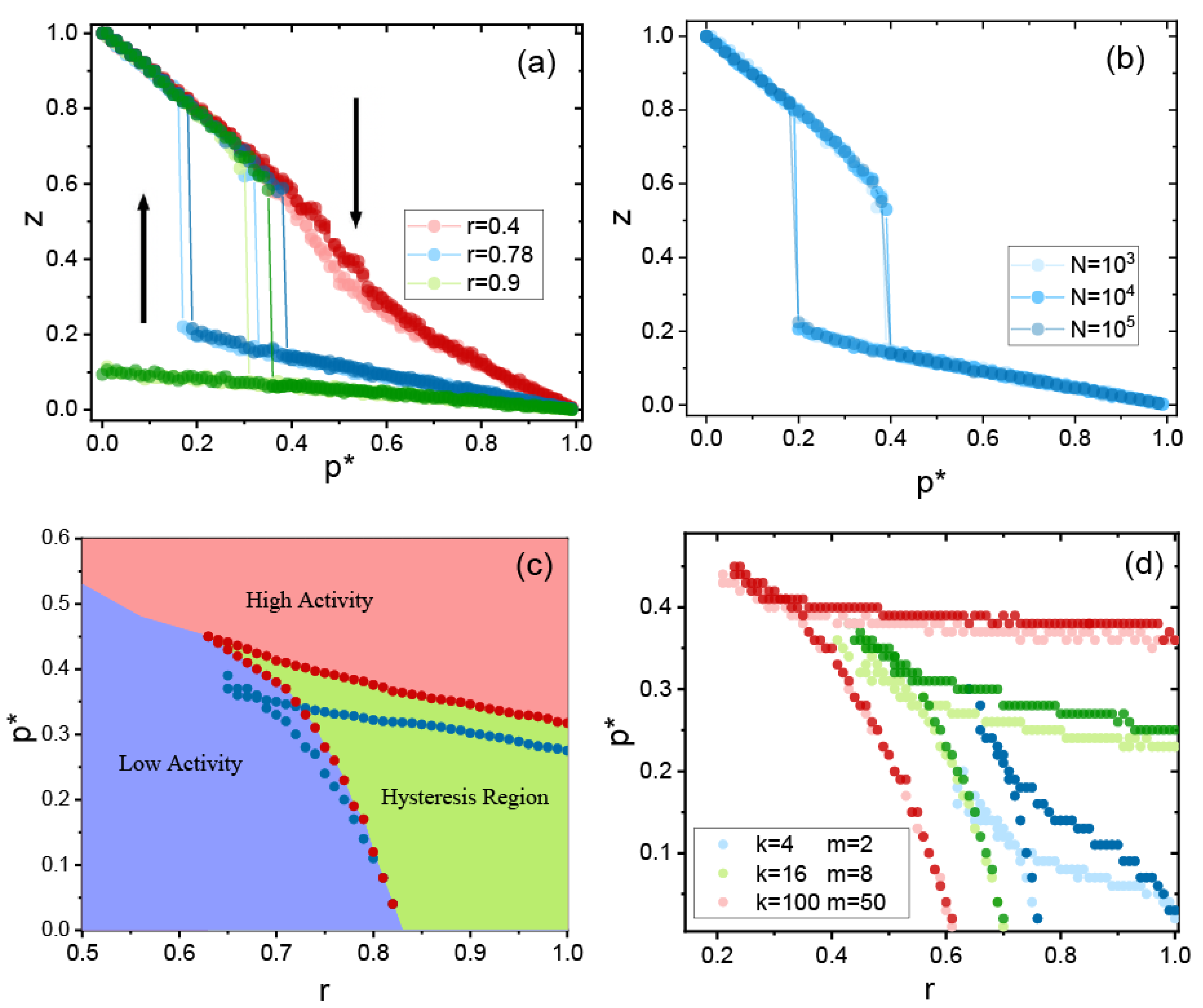
We perform numerical simulations for random regular (RR) networks with a Kronecker delta degree distribution ($P\left(k\right)={\delta }_{k,<k>}$), Erdos-Rényi (ER) networks with a Poissonian degree distribution ($P\left(k\right)=\frac{e^{-<k>}<k{>}^k}{k!}$) [26], and Scale-Free (SF) networks with a power law degree distribution ($P\left(k\right)\sim k^{-\lambda }$) [27]. Here, $<k>$ is the average degree of the network, and $\lambda$ is the power law index of SF network. In simulations, without a loss of generality, we adopt the recovery times $\tau =100$ and ${\tau }^{{}^{\prime }}=1$. In view of the relationship between p and $\tau$ in ref. [12], we define the parameter $p^{*}=1-e^{-p\tau }$ as representing the internally failed nodes. Figure 2 shows a fraction $z\left(t\right)$ of the average active nodes for the RR network with an average degree $<k>=10$ as a function of t at the same $p^{*}$ but a different dynamic process. We set $m=4,r=0.78$, and a fraction $p=0.3$ of nodes are initially localised failure.

Since the system dynamically alternates between localised failure and spontaneous recovery at every step, this dynamic process with memory means the previous stable state will affect the next system state. $p^{*}$ denotes the the average fraction of internally failed nodes, and it can change from 0 to 1 and then turn to change from 0 to 1. Since the initial state under each $p^{*}$ depends on the final stable state of the previous $p^{*}$, the same $p^{*}$ at a different direction may have a different result. As shown in Figure 2, we simulated the results of the RR network for all $p^{*}$ with a step size of 0.01. In Figure 2a, $p^{*}$ = 0.3 ($p^{*}$ changes from 0 to 1) depends on the final stable state of $p^{*}$ = 0.29, but the second $p^{*}$ = 0.3 ($p^{*}$ changes from 1 to 0) shown in Figure 2b depends on the final stable state of $p^{*}$ = 0.31. The result in this figure shows that the active nodes changed over time in the increasing direction, and the eventually stable fraction is close to 0.69. However, for the decreasing direction, $z\left(t\right)$ tends to be stable at around 0.17, and it is very different from the previous one. Due to the memory nature during system failure and recovery, the same $p^{*}$ value at different directions leads to different states, respectively.

These results highlight that the fraction of active nodes at different failure stages displays a diver’s steady state even though all the parameters are the same due to system’s damaged memory. In Figure 3a, we show the fraction of the average active nodes z in a steady state as a function of $p^{*}$ at three different r values for the RR network with $<k>=10$ and $m=4$ under a localised attack. As $r=0.4$, the system has weak external failures, and the fraction of average active nodes z shows continuous phase behaviours for the increasing or decreasing directions of $p^{*}$. As r equals $0.78$ or $0.9$ with strong external failures, the system z both shows dis-continuous phase behaviours for the increasing or decreasing directions of $p^{*}$, in which the jump thresholds are different values. The hysteresis shown in Figure 3a is the characteristic feature of a first-order phase transition. Comparing the dynamics under RA (light symbols) and LA (dark symbols), it can easily be found that the critical point of LA is a bit larger than RA, which means that the RR network is more resilient under LA than RA. It is easy to explain because, for LA, only the internal failure nodes on the outer shell of the attacked hole will affect the external failure of nodes, but for RA, all internal failure nodes will affect the remaining active nodes. These results are also consistent with the results of a single static RR network [22]. In order to reduce the impact of the number of nodes, we also compare the average fraction of active nodes z when $r=0.78$ under LA, which is shown in Figure 3b. The results imply that the impact of the network’s finite size on the RR network is almost negligible, and the jump points are almost the same for different $N={10}^3,{10}^4,{10}^5$ when $r=0.78$. By repeating this procedure for different r values, we obtain the two-parameter ($r,p^{*}$) phase diagram shown in Figure 3c. The jump points split the phase diagram into three regions: one is the high-activity region (purple), which means there are more active nodes, the other one is the low-activity region (pink), and the hysteresis region (green) is between the other two regions. One can observe that the initial condition (fraction of failed nodes) determines the final stable state, and if the fraction of failed nodes is smaller than one in the unstable state, the dynamic will reach the high-activity region. However, if there are more failed nodes, it will be easier to reach the low-activity region. Figure 3d compares the dynamic behaviours under RA and LA, and the critical value of an LA is always larger than the one under an RA. Under the same conditions, whether it is a static or a dynamic recovery for the RR network, an LA always makes the network more robust compared to an RA. We also study the resilience of RR with different parameters, as shown in Figure 3d. The system shows more resilience under the LA (dark points) in contrast to RA (light points). In addition, the average degree $<k>$ and the number of active neighbours m both affect the width of the hysteresis region. The larger average degree, the wider the hysteresis region displayed by the system. These results will be helpful for studying the spontaneous recovery in real systems under LA.

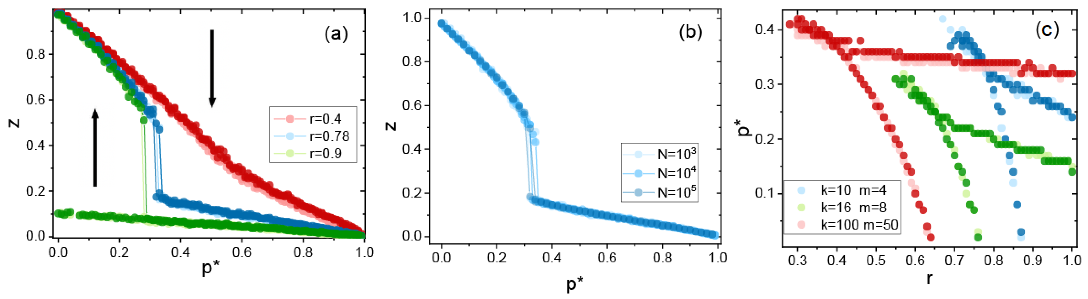
Next, the dynamic recovery network in an ER network is studied. Figure 4a shows z as a function of $p^{*}$, and the results imply that these two simulated results under RA (light symbol) and LA (dark symbol) almost overlap. Similar to the RR network, there also exists discontinuous phase transitions, and the probability of external failure not only affects the value of the critical point but also affects the hysteresis region. We also compare the influence of the size of the ER network in Figure 4b. The fractions of active nodes as $r=0.78$ for different N are almost same. As the parameters ($r,p^{*}$) change, the different initial node states can evolve into the hysteresis region, as shown in Figure 4c. Not surprisingly, the phase diagrams of the ER network under these two failure mechanisms almost show the same behaviours. This phenomena can also be found in a single static ER network [22].

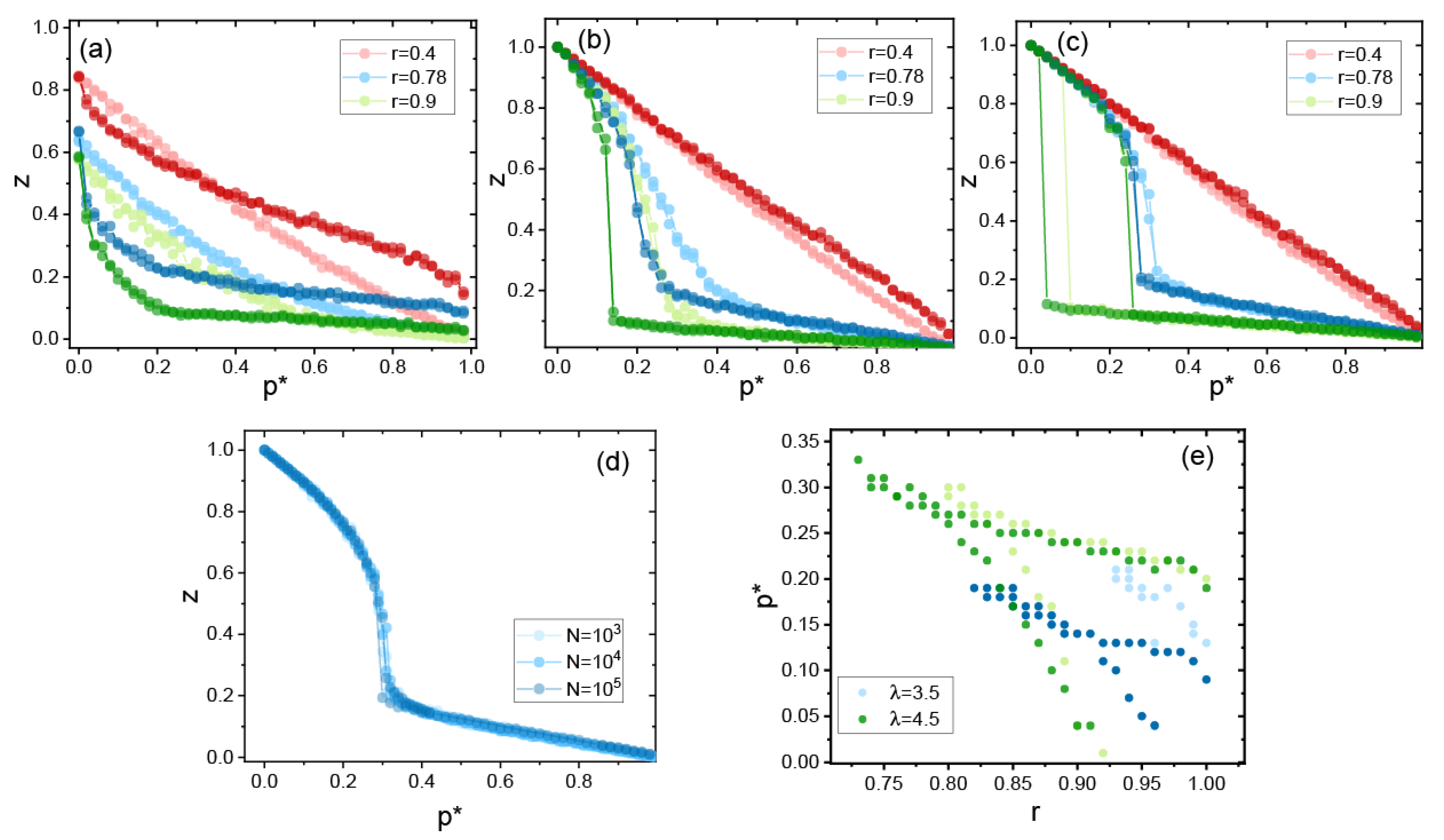
Scale-free networks also have similar phase transition behaviours, which are shown in Figure 5a–c. However, when the power index is $\lambda =2.5$, the results both show second-order continuous phase transition behaviours under RA and LA. The proportion of internally failed nodes under different failure modes affects the proportion of average active nodes z. As the internally failed nodes become smaller, the network system shows strong resilience under RA (light symbols) than LA (dark symbols). However, as $p^{*}$ increases, the network system under LA shows more resilience than RA. With the increase of $\lambda$, there is a first-order jump phenomenon for larger r values. To compare the influence of the network size, we simulate the SF network with $\lambda =4.5$ and $r=0.78$ in Figure 5d. It can be found that there is almost no effect on the jump point. Figure 5e shows the two regions for different $\lambda$ values. When $\lambda =2.5$, there are no jump points. However, when $\lambda =3.5,4.5$, they have similar results with RR and ER networks and show the phase-flipping phenomena.

3. Conclusions

Here, we study the dynamical behaviours of network systems, including RR, ER, and SF networks, by considering the dynamic spontaneous recovery after a more realistic localised attack. After the internal failure, the node also has a probability to become inactive if it does not have enough active neighbours, which is the external failure mechanism. We assume that each node can be active after a certain period of time, if it has failed internally or externally. From comparing with the network under an internally random attack, we found that the RR network was more resilient under an LA than an RA. This is because, under LA, only the outer shell of the attacked hole will affect the external failure rather than the all of the internally failed nodes under RA. For the ER network, it has the same dynamic resilience for both attacking strategies, and this result is the same as the static ER network under these two types of failures [22]. However, for the SF network, it has more resilience under RA and LA for a larger power index. The dynamics of these three networks show both the phase-flipping phenomena and the proportion of the active nodes that switch back and forth between high network activity and low network activity. We also find that a strong hysteresis behaviour exists analogous to phase transitions near a critical point for these networks. Additionally, the results also imply that the system resilience mainly depends on the proportion of internally failed nodes for both attacking strategies. These findings show a potential application for repairing damaged real systems. The code has been shared in GitHub, and the link is https://github.com/wwwfanang/Local-Recovery-Network.git accessed on 1 August 2021.

References

- Borgatti, S.P.; Mehra, A.; Brass, D.J.; Labianca, G. Network analysis in the social sciences. Science 2009, 323, 892–895. [Google Scholar] [CrossRef] [Green Version]
- Colizza, V.; Barrat, A.; Barthélemy, M.; Vespignani, A. The role of the airline transportation network in the prediction and predictability of global epidemics. Proc. Natl. Acad. Sci. USA 2006, 103, 2015–2020. [Google Scholar] [CrossRef] [PubMed] [Green Version]
- Cohen, R.; Erez, K.; Ben-Avraham, D.; Havlin, S. Breakdown of the internet under intentional attack. Phys. Rev. Lett. 2001, 86, 3682. [Google Scholar] [CrossRef] [PubMed] [Green Version]
- Cohen, R.; Erez, K.; Havlinl, S.; Newman, M.; Barabási, A.-L.; Watts, D.J. Resilience of the internet to random breakdowns. In The Structure and Dynamics of Networks; Princeton University Press: Princeton, NJ, USA, 2011; pp. 507–509. [Google Scholar]
- Callaway, D.S.; Newman, M.E.; Strogatz, S.H.; Watts, D.J. Network robustness and fragility: Percolation on random graphs. Phys. Rev. Lett. 2000, 85, 5468. [Google Scholar] [CrossRef] [Green Version]
- Gallos, L.K.; Cohen, R.; Argyrakis, P.; Bunde, A.; Havlin, S. Stability and topology of scale-free networks under attack and defense strategies. Phys. Rev. Lett. 2005, 94, 188701. [Google Scholar] [CrossRef] [Green Version]
- Dong, G.; Wang, F.; Shekhtman, L.M.; Danziger, M.M.; Fan, J.; Du, R.; Liu, J.; Tian, L.; Stanley, H.E.; Havlin, S. Optimal resilience of modular interacting networks. Proc. Natl. Acad. Sci. USA 2021, 118, e1922831118. [Google Scholar] [CrossRef]
- Li, D.; Fu, B.; Wang, Y.; Lu, G.; Berezin, Y.; Stanley, H.E.; Havlin, S. Percolation transition in dynamical traffic network with evolving critical bottlenecks. Proc. Natl. Acad. Sci. USA 2015, 112, 669–672. [Google Scholar] [CrossRef] [Green Version]
- Dickison, M.; Havlin, S.; Stanley, H.E. Epidemics on interconnected networks. Phys. Rev. E 2012, 85, 066109. [Google Scholar] [CrossRef] [Green Version]
- Shang, Y. Attack robustness and stability of generalized k-cores. New J. Phys. 2019, 21, 093013. [Google Scholar] [CrossRef]
- Liu, Y.; Sanhedrai, H.; Dong, G.; Shekhtman, L.M.; Wang, F.; Buldyrev, S.V.; Havlin, S. Efficient network immunization under limited knowledge. Natl. Sci. Rev. 2021, 8, nwaa229. [Google Scholar] [CrossRef]
- Majdandzic, A.; Podobnik, B.; Buldyrev, S.V.; Kenett, D.Y.; Havlin, S.; Stanley, H.E. Spontaneous recovery in dynamical networks. Nat. Phys. 2014, 10, 34–38. [Google Scholar] [CrossRef]
- Shang, Y. Percolation of attack with tunable limited knowledge. Phys. Rev. E 2021, 103, 042316. [Google Scholar] [CrossRef] [PubMed]
- Majdandzic, A.; Braunstein, L.A.; Curme, C.; Vodenska, I.; Levy-Carciente, S.; Stanley, H.E.; Havlin, S. Multiple tipping points and optimal repairing in interacting networks. Nat. Commun. 2016, 7, 1–10. [Google Scholar] [CrossRef] [Green Version]
- Dong, G.; Fan, J.; Shekhtman, L.M.; Shai, S.; Du, R.; Tian, L.; Chen, X.; Stanley, H.E.; Havlin, S. Resilience of networks with community structure behaves as if under an external field. Proc. Natl. Acad. Sci. USA 2018, 115, 6911–6915. [Google Scholar] [CrossRef] [Green Version]
- Zeng, G.; Gao, J.; Shekhtman, L.; Guo, S.; Lv, W.; Wu, J.; Liu, H.; Levy, O.; Li, D.; Gao, Z.; et al. Multiple metastable network states in urban traffic. Proc. Natl. Acad. Sci. USA 2020, 117, 17528–17534. [Google Scholar] [CrossRef] [PubMed]
- Yang, Z.; Su, Z.; Liu, S.; Liu, Z.; Ke, W.; Zhao, L. Evolution features and behavior characters of friendship networks on campus life. Expert Syst. Appl. 2020, 158, 113519. [Google Scholar] [CrossRef]
- Muro, M.A.D.; Rocca, C.E.L.; Stanley, H.E.; Havlin, S.; Braunstein, L.A. Recovery of interdependent networks. Sci. Rep. 2016, 6, 1–11. [Google Scholar]
- Podobnik, B.; Jusup, M.; Tiganj, Z.; Wang, W.-X.; Buldú, J.M.; Stanley, H.E. Biological conservation law as an emerging functionality in dynamical neuronal networks. Proc. Natl. Acad. Sci. USA 2017, 114, 11826–11831. [Google Scholar] [CrossRef] [PubMed] [Green Version]
- Böttcher, L.; Andrade, J.; Herrmann, H.J. Targeted recovery as an effective strategy against epidemic spreading. Sci. Rep. 2017, 7, 1–7. [Google Scholar] [CrossRef] [PubMed] [Green Version]
- Shang, Y. Localized recovery of complex networks against failure. Sci. Rep. 2016, 6, 1–10. [Google Scholar] [CrossRef] [Green Version]
- Shao, S.; Huang, X.; Stanley, H.E.; Havlin, S. Percolation of localized attack on complex networks. New J. Phys. 2015, 17, 023049. [Google Scholar] [CrossRef]
- Liu, Y.; Zhao, C.; Yi, D.; Stanley, H.E. Robustness of partially interdependent networks under combined attack. Chaos Interdiscip. Nonlinear Sci. 2019, 29, 021101. [Google Scholar] [CrossRef] [PubMed] [Green Version]
- Yuan, X.; Shao, S.; Stanley, H.E.; Havlin, S. How breadth of degree distribution influences network robustness: Comparing localized and random attacks. Phys. Rev. E 2015, 92, 032122. [Google Scholar] [CrossRef] [PubMed] [Green Version]
- Yuan, X.; Dai, Y.; Stanley, H.E.; Havlin, S. k-core percolation on complex networks: Comparing random, localized, and targeted attacks. Phys. Rev. E 2016, 93, 062302. [Google Scholar] [CrossRef] [Green Version]
- Gilbert, E.N. Random graphs. Ann. Math. Stat. 1959, 30, 1141–1144. [Google Scholar] [CrossRef]
- Albert, R.; Barabási, A.-L. Statistical mechanics of complex networks. Rev. Mod. Phys. 2002, 74, 47. [Google Scholar] [CrossRef] [Green Version]
Figure 1.
Schematic illustration of the dynamic recovery process under an LA. At time , after these four steps, the network changed into the fourth network in the first row. Nodes 1 and 3 are suffering internal failure, but node 3 has recovered one time (l = 1), while node 1 just internally failed the last time (). Additionally, node 2 is suffering an external failure (). At time t, nodes 4 and 5 are chosen to internally fail, and then nodes 7 and 8 only have one active neighbour, so they externally fail. Node 1, which internally fails at time , can recover one time (), and node 3 has achieved , so it can be active again, and the edge between nodes 3 and 6 can also be active. Finally, node 2 reaches the time required for external recovery, and it becomes active (). Next time, two nodes will be locally chosen again, and the node still belonging to the internal failure state can fail again, such as node 1 in the first network in the third row since its l changed to 0 again. Then, the process occurs repeatedly.
Figure 2.
Model dynamical recovery on the RR network for with . (a) The high activity steady state ( is about 0.685) for the increasing direction of (from 0 to 1). (b) The low activity steady state ( is about 0.17) for the decreasing direction of (from 1 to 0).
Figure 3.
Phase diagrams of the RR network. (a) Simulation results of the average fraction of nodes for three different r values under LA (dark symbols) and RA (light symbols). The parameters for the RR network are and . (b) Simulation results of the average fraction of nodes for three different r values under LA for different N with , and . (c) The phase diagram in model parameters () exhibits two kinds of phase transition behaviours. Low- and high-activity correspond to the cases where the fraction of active nodes of the stationary state is small or large, respectively. Red points are the dividing points between the hysteresis region and high/low-activity regions under LA. Additionally, two bunches of red points merge at a critical point located at (). Blue points are the similar results under RA. (d) Jump points for different parameters. Light points are RA, and dark points are LA. Simulation results have been averaged over 1000 network realisations.
Figure 4.
Phase diagrams of the ER network. (a) Simulation results of the average fraction of nodes for three different r, and the parameters are and . (b) Simulation results of the average fraction of nodes for three different r values under LA for different N with and . (c) The jump point for different parameters. Dark and light symbols denote LA and RA, respectively. Simulation results have been averaged over 1000 network realisations.
Figure 5.
Phase diagrams of the SF network. (a–c) Simulation results of the average fraction of nodes for three different values of r, and the parameters are and , and in proper order, . (d) Simulation results of the average fraction of nodes for three different r values under LA for different N with and . (e) Jump points for different values. Dark and light symbols denote LA and RA, respectively. Simulation results have been averaged over 1000 network realisations.
Publisher’s Note: MDPI stays neutral with regard to jurisdictional claims in published maps and institutional affiliations. |
© 2021 by the authors. Licensee MDPI, Basel, Switzerland. This article is an open access article distributed under the terms and conditions of the Creative Commons Attribution (CC BY) license (https://creativecommons.org/licenses/by/4.0/).
Share and Cite
MDPI and ACS Style
Wang, F.; Dong, G.; Tian, L. Dynamical Recovery of Complex Networks under a Localised Attack. Algorithms 2021, 14, 274. https://0-doi-org.brum.beds.ac.uk/10.3390/a14090274
AMA Style
Wang F, Dong G, Tian L. Dynamical Recovery of Complex Networks under a Localised Attack. Algorithms. 2021; 14(9):274. https://0-doi-org.brum.beds.ac.uk/10.3390/a14090274
Chicago/Turabian StyleWang, Fan, Gaogao Dong, and Lixin Tian. 2021. "Dynamical Recovery of Complex Networks under a Localised Attack" Algorithms 14, no. 9: 274. https://0-doi-org.brum.beds.ac.uk/10.3390/a14090274
Note that from the first issue of 2016, this journal uses article numbers instead of page numbers. See further details here.