Feature Selection for High-Dimensional Datasets through a Novel Artificial Bee Colony Framework

Abstract

There are generally many redundant and irrelevant features in high-dimensional datasets, which leads to the decline of classification performance and the extension of execution time. To tackle this problem, feature selection techniques are used to screen out redundant and irrelevant features. The artificial bee colony (ABC) algorithm is a popular meta-heuristic algorithm with high exploration and low exploitation capacities. To balance between both capacities of the ABC algorithm, a novel ABC framework is proposed in this paper. Specifically, the solutions are first updated by the process of employing bees to retain the original exploration ability, so that the algorithm can explore the solution space extensively. Then, the solutions are modified by the updating mechanism of an algorithm with strong exploitation ability in the onlooker bee phase. Finally, we remove the scout bee phase from the framework, which can not only reduce the exploration ability but also speed up the algorithm. In order to verify our idea, the operators of the grey wolf optimization (GWO) algorithm and whale optimization algorithm (WOA) are introduced into the framework to enhance the exploitation capability of onlooker bees, named BABCGWO and BABCWOA, respectively. It has been found that these two algorithms are superior to four state-of-the-art feature selection algorithms using 12 high-dimensional datasets, in terms of the classification error rate, size of feature subset and execution speed.

1. Introduction

Due to the rapid development of data acquisition technology, a great deal of digital information is becoming more easily collected and included in datasets. However, not all features in datasets are useful for a target problem. In other words, there are many redundant and irrelevant features in high-dimensional datasets, so feature selection (FS) is used as a vital data preprocessing step in data mining and machine learning [1]. However, FS is an NP-hard problem. For an n-dimensional dataset, there are 2n feature subsets, which is difficult to solve with an exhaustive method. With a good FS method, we can not only get higher classification accuracy, but also reduce the complexity of calculation. In order to improve the search efficiency of FS algorithms, many scholars propose algorithms, which can be roughly divided into three types: filter method, wrapper method and embedded method [2]. Among them, the wrapper method is widely used because of its good classification ability. Therefore, this paper studies the wrapper FS method.

The wrapper approach mainly consists of three parts: classifiers, feature subset evaluation criteria and search techniques [3]. Among them, an effective search technique is crucial for the performance of FS algorithms. It is worth mentioning that meta-heuristic methods, such as the artificial bee colony (ABC) algorithm [4], the particle swarm optimization (PSO) algorithm [5], the differential evolution (DE) algorithm [6], the grey wolf optimization (GWO) algorithm [7], the whale optimization algorithm (WOA) [8], and many other algorithms [9] have provided good search strategies for the FS task. Unlike the exact search mechanisms, meta-heuristic methods exhibit superior performance, as they do not generate all possible solutions for a given task. Meta-heuristic algorithms have exploration and exploitation abilities, and the trade-off between both abilities is very important for the performance of these algorithms. The exploration acts to discover various unknown regions for more potential solutions, while the exploitation attempts to generate better solutions on the basis of the information provided by existing solutions. In some meta-heuristic search techniques, the ability of exploration is stronger, while in others, the exploitation performs better [10,11]. Exploring the search region and exploiting the best solution are two contradictory criteria that must be considered simultaneously when designing a good meta-heuristic algorithm. The key to improving an algorithm is to achieve a good balance between exploration and exploitation [3,12].

The ABC algorithm is an optimization algorithm that is inspired by the foraging behavior of a honey bee swarm. ABC has been successfully applied to various optimization problems due to its good properties, such as few parameters to control, its high flexibility, and its strong global search ability [11]. However, ABC converges slowly because of the absence of a strong local exploitation ability [10,13]. From the above considerations, we propose a new framework to enhance the exploitation performance of the ABC algorithm, so as to realize a trade-off between the exploration and exploitation capabilities of the FS method, and raise the optimization efficiency and effectiveness. The contributions of this paper are as follows:

(1)

In order to trade off the exploitation and exploration abilities of ABC, we use operators with strong exploitation abilities to enhance the exploitation ability in the phase of onlooker bee;

(2)

This paper analyzes the functional behavior of the scout bee phase and finds that this phase may be redundant while dealing with high-dimensional FS problems, and so eliminating this phase can reduce the computational time of the algorithm;

(3)

The proposed framework is designed as a general framework that can be used to adapt many ABC variants for the FS problems.

The remainder of this paper is illustrated as follows: Section 2 briefly describes the related works of the ABC algorithm. In Section 3, the original ABC algorithm is introduced and analyzed. Section 4 presents the details of our proposed approach. In Section 5, comparisons of the experimental results are presented and discussed. The proposed algorithms are further analyzed in Section 6. At last, the conclusions and future work are outlined in Section 7.

2. Related Works

Recently, meta-heuristic algorithms have attracted the attention of many scholars. These algorithms can be used to solve many real engineering tasks, such as path planning [14,15,16], feature selection [17,18,19], function optimization [20,21,22], and the traveling salesman problem [23,24,25]. Although various meta-heuristics have been developed to deal with FS over the years, the significant increase in data dimensionality brings great challenges; therefore, it is worth continuing looking for effective strategies to make meta-heuristic algorithms perform better for high-dimensional FS problems [26].

ABC was proposed in 2005 by Karaboga group to optimize algebraic problems [27]. Single-objective ABC was first used to address the FS problem in 2012 [18,28]. Almost all meta-heuristic algorithms have the problem of an imbalance between exploration and exploitation [29], and the ABC algorithm is no exception. There are a lot of studies on the ABC algorithm, seeking to improve its exploitation capability. To accelerate the convergence speed of the ABC algorithm, Chao et al. [30] proposed the KnABC algorithm, which introduced Knee Points into the employed bee phase and onlooker bee phase. The results show that this algorithm has a significant effect on reducing the number of features and increasing the classification accuracy. Shunmugapriya et al. [31] utilized the ACO algorithm for colony initialization, and took the initialization results as the food sources of the ABC algorithm for further optimization so as to integrate the ACO and ABC algorithms; the resulting algorithm’s performance was better than that of ABC or ACO alone. Djellali et al. [10] proposed two hybrid ABC algorithms, i.e., ABC-PSO and ABC-GA, which integrate the PSO algorithm and GA algorithm into the framework of the original ABC algorithm in different bee phases, respectively. The experimental results showed that ABC-GA obtained better results than some other existing methods. Shunmugapriya et al. [32] proposed the EABC-FS algorithm, in which the employed bees and onlooker bees made full use of the best solutions in the current swarm to enhance the exploitation ability of the ABC algorithm. The experimental results showed that the performance of the algorithm achieved by introducing such fusion strategies was greatly improved. Moreover, many other studies have shown that the ABC algorithm faces the problem of an insufficient exploitation ability, which results in it becoming trapped in a local optimum and having a low convergence speed [28,33].

Although the above-mentioned hybrid variants of the ABC algorithm have achieved promising performance, they do not deeply analyze the exploitation and exploration abilities in different bee phases of the overall framework. Moreover, few of these algorithms have been developed for high-dimensional FS. Therefore, this paper proposes a novel exploration and exploitation trade-off ABC algorithm by modifying the original overall framework, and applies it to high-dimensional datasets. This new framework strengthens the exploitation ability in the onlooker bee phase by using operators with high exploitation capacities. Additionally, the function of scout bees is discussed in detail, and verified by experiments.

3. Introduction and Analysis of ABC Algorithm

The ABC algorithm is a kind of swarm intelligence (SI) algorithm that simulates the honey-gathering behavior of a bee swarm. This algorithm includes three types of bees: employed bees, onlooker bees and scout bees. Each food source corresponds to a solution to the given task, and the fitness of the solution indicates the quality of the food source. The overall process of the ABC algorithm is as follows [34].

First of all, it initializes a population of size SN randomly. This is calculated by Equation (1):

$$x_{id}=x_d^{min}+r*\left(x_d^{max}-x_d^{min}\right)$$

(1)

where i = 1, 2,…, SN, d = 1, 2,…, D. SN is the number of food sources. D is the dimensionality of the search space. Additionally, the number of employed bees or onlooker bees is equal to the number of food sources. r is a random number in [0, 1], distributed uniformly. $x_d^{min}$ and $x_d^{max}$ represent the maximum and minimum values of the dth dimension feature, respectively. After initialization, the bees begin to search.

(1)

Employed bee phase: According to Equation (2), a new food source is produced around the current food source, as follows:

$$x_{id}^{\prime }=x_{id}+{\phi }_{id}*\left(x_{id}-x_{kd}\right)$$

(2)

where ${\phi }_{id}$ is a random number within [−1,1]. $x_{id}$ and $x_{kd}$ represent the dth dimension feature of $x_i$ and $x_{\mathrm{k}}$, respectively. $x_{id}^{\prime }$ is compared with $x_{id}$, and if the fitness of $x_{id}^{\prime }$ is superior to $x_{id}$, $x_{id}$ is replaced by $x_{id}^{\prime }$ for entry into the next step, and its counter is reset to 0. Otherwise, $x_{id}$ is retained for entry into the next step, and its counter increases by 1.

(2)

Onlooker bee phase: Every onlooker bee selects a food source depending on the probability value $p_i$ via the roulette-wheel scheme. $p_i$ is associated with the food resource information given by the employed bee. The value of $p_i$ is generated by Equation (3).

$$p_i=\frac{fi{t}_i}{{{\displaystyle \sum }}_{i=1}^{SN}fi{t}_i}$$

(3)

where ${fit}_i$ is the fitness value of solution $x_i$. Each selected food source is updated using Equation (2).

(3)

Scout bee phase: If the counter of a food source is greater than or equal to the preset number of trials, then this food source is discarded. The value of the preset number of trials is usually called the limit for abandonment. If a food source is abandoned, then the scout bee translated from the employed bee will regenerate a food source via Equation (1) to replace the food source that is abandoned.

In the ABC algorithm, the employed bees are in charge of finding viable solutions throughout the search area, and providing the onlooker bees with food information. Based on the food information, the onlooker bees search new food sources near to the existing found food sources. In the updating process of the onlooker bee phase, the same updating formula (Equation (2)) is used to update the population as in the employed bee phase. As we can see from the above, the ABC algorithm does not take advantage of the elitism principle. Both the employed bees and onlooker bees use Equation (2) to obtain new food resources, as it has a powerful global search ability, but its search efficiency is low and its exploitation ability is not optimal. The roulette-wheel scheme can make food sources with higher fitness values easier to select, and the use of the roulette-wheel scheme in the onlooker bee phase can strengthen the exploitation ability, but this exploitation ability is far less strong than its powerful exploration ability. Therefore, as Hong and Ahn [35] have pointed out, the exploitation level of the onlooker bee phase should increase. In addition, the scout bee phase not only reduces the probability of falling into the local optimum, but it also reduces the rate of convergence. Under the action of the scout bees, the optimal solution may also be discarded [34]. Therefore, the ABC algorithm has an outstanding exploration capacity but inefficient exploitation. This imbalance renders the ABC algorithm unable to reach a better solution, because the convergence is too slow.

4. Proposed Algorithm for Feature Selection

4.1. The Proposed Framework

A meta-heuristic algorithm having a balance between exploration and exploitation ability has a great impact on its performance. For an algorithm with good exploration ability, we can enhance its exploitation ability by introducing operators with strong exploitation ability so as to regain the balance between exploration and exploitation abilities. Based on the analysis in Section 3, this paper presents a novel ABC framework. There are three points in the description of the framework:

(1)

The employed bee phase of the ABC algorithm is retained so that it can explore the search space widely and avoid reaching the local optimum;

(2)

The updating mode of the ABC algorithm’s onlooker bee phase is changed to the new updating strategy, as inspired by other algorithms with more powerful exploitation capacities. The searching scheme of these algorithms with powerful exploitation abilities is introduced as an operator. According to our observation, higher diversity in the bee swarm can help the algorithm to find more potential search space, but after a certain period, the solutions should converge and approach optimal solutions with reductions in colony diversity. We believe that applying operators with strong exploitation abilities to the optimization process can reduce the diversity of the algorithm in the late stage, and bring about a higher convergence speed. Therefore, the introduction of operators with powerful exploitation abilities can help our novel ABC framework find better solutions;

(3)

The scout bee phase is removed, because the exploration ability of the scout bee phase will increase the diversity of the algorithm during the later period. Moreover, the scout bee phase will waste the execution time, and consume computational resources and memory during the calculation process.

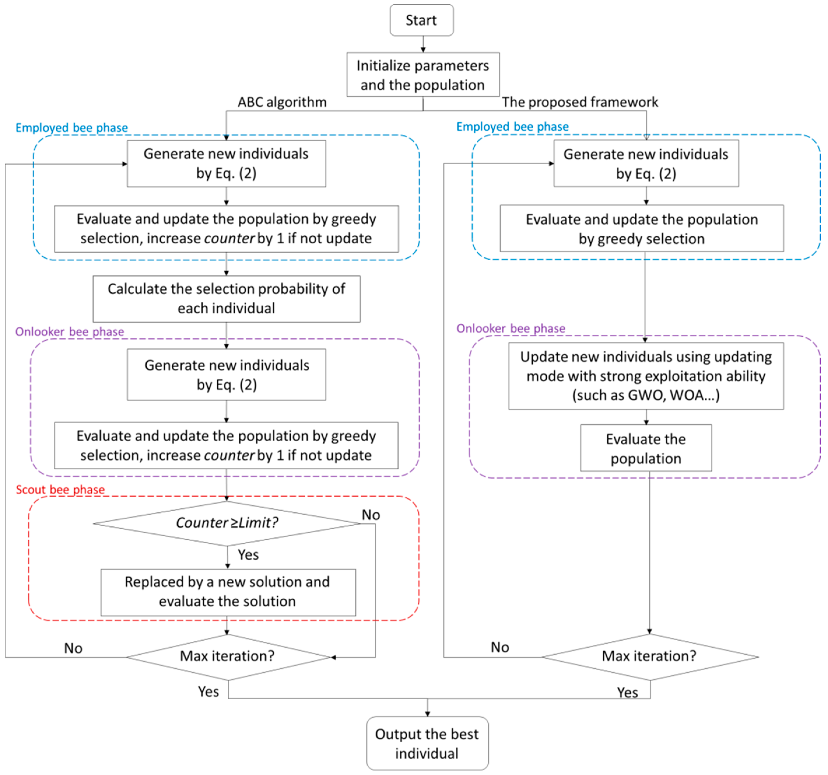
Figure 1 illustrates our proposed framework and its differences from the processes of the original ABC algorithm. Overall, the two methods utilize the same updating mechanism in the employed bee phase. However, without the scout bee phase, our method does not need to compute the value of the counter throughout the algorithm. Since the onlooker bee phase in our method is updated by the operators of an algorithm with strong exploitation abilities, we do not use roulette-wheel selection, so we do not need to calculate the selection probability of each individual.

FS is, in essence, an optimization problem in a binary searching space. The value of each element of the solutions is limited to 0 or 1 [36]. However, the ABC algorithm originally proposed is used in continuous space. To adapt our proposed ABC framework to FS, we need to transform the continuous values to binary values. This transformation is fulfilled by Equation (4).

$$x{b}_{id}=\{\begin{array}{cc}1& if \mathrm{r}<\mathrm{sigmoid}\left(x_{id}\right)\\ 0& otherwise\end{array}$$

(4)

where r is a random value in [0, 1]. The function of $sigmoid\left(x\right)$ is formulated as in Equation (5):

$$sigmoid\left(x\right)=\frac{1}{1+exp(-10*\left(x-0.5\right))}$$

(5)

4.2. Abandonment of Scout Bee Phase to Reduce the Exploration Capacity

As the last phase of the ABC algorithm, the scout bee abandons any individual that has not changed for a long time, and then creates a new individual to replace the abandoned individual. This phase has certain exploration advantages for the algorithm. However, it has been proven [34] that the scout bee phase is not active in processing high-dimensional tasks, and runs the risk of missing local optimal solutions due to its exploration ability; as such, we have removed this phase. In the following experiments, we analyze the influence of removing the scout bee phase on the diversity and convergence ability of the algorithm.

4.3. Enhancement of Exploitation—Illustrative Example with GWO and WOA

The original ABC algorithm has a low exploitation capacity, especially in the onlooker bee phase. The enhancement of the exploitation capacity in this phase is the most vital factor to regaining the trade-off between exploitation and exploration in the whole procedure of the ABC algorithm. There are many algorithms that have powerful exploitation capacities, such as the GWO algorithm and WOA algorithm. Compared with other algorithms, the GWO algorithm and WOA algorithm make full use of the information related to excellent individuals in the updating process, which gives them powerful exploitation abilities. As such, we take these two algorithms as examples. In our research, we fuse each algorithm as an operator into the onlooker bee phase, and replace the updating mode of the original ABC algorithm in the same phase to enhance the exploitation capacity of our whole framework.

In the GWO algorithm, the grey wolves are divided into four hierarchies, namely, alpha (α), beta (β), delta (δ) and omega (ω). In solving optimization problems, the α wolf is the best solution, the β and δ wolves are the second- and third-best solutions, respectively, while the ω wolves are the remaining candidates. The α, β, and δ wolves lead the wolf pack to search for prey. The position of each wolf is given as follows:

$$\begin{array}{c}{D}_{\alpha }=|C_1*X_{\alpha }-X|,\\ D_{\beta }=|C_2*X_{\beta }-X|,\\ D_{\delta }=|C_3*X_{\delta }-X|\prime \end{array}$$

(6)

$$\begin{array}{c}{X}_1=X_{\alpha }-A_1*D_{\alpha },\\ X_2=X_{\beta }-A_2*D_{\beta },\\ X_3=X_{\delta }-A_3*D_{\delta },\end{array}$$

(7)

$$X(t+1)=\frac{X_1+X_2+X_3}{3}$$

(8)

where $X_{\alpha }$, $X_{\beta }$ and $X_{\delta }$ refer to the position vectors of α, β and δ, respectively. $D_{\alpha }$, $D_{\beta }$ and $D_{\delta }$ denote the distance between the prey (α, β, δ) and the current wolf, respectively. t indicates the current iteration. $A=2a*r_1-a$, $C=2*r_2$, $r_1$ and $r_2$ are random numbers in [0, 1] that are distributed uniformly. The value of $a$ decreases linearly from 2 to 0 as the number of cycles increases. The three best solutions are used to be learnt from during the updating process of the GWO algorithm, which gives it a strong exploitation ability [7,37,38].

The WOA algorithm is also an SI algorithm, which employs the current optimal solution as the prey. The search agents update their positions based on the best solution. The mathematical model is described by the equations:

$$X(t+1)=\{\begin{array}{cc}{X}_p\left(t\right)-A*D& p<0.5,\left|A\right|<1\\ D^{\prime }*e^{bl}*\cos (2\pi l)+X_p\left(t\right)& p\ge 0.5\end{array}$$

(9)

$$\begin{array}{cc}X(t+1)=X_{\mathrm{rand}}\left(t\right)-A*D^{″}& p<0.5,\left|A\right|\ge 1\end{array}$$

(10)

where $X_p\left(t\right)$ is the best search agent, $X_{\mathrm{rand}}\left(t\right)$ is a random position vector, b is a manually determined constant, and l is a random number in [–1,1]. The equations for calculating $D$, $D^{\prime }$ and $D^{″}$ are as follows:

$$\begin{array}{c}D=\left|C*X_p\left(t\right)-X\left(t\right)\right|,\\ D^{\prime }=\left|X_p\left(t\right)-X\left(t\right)\right|,\\ D^{″}=\left|C*X_{\mathrm{rand}}\left(t\right)-X\left(t\right)\right|\end{array}$$

(11)

where A and C are calculated in the same way as above. The process of updating the WOA algorithm selects the best solution for learning, which makes the exploitation ability of the algorithm more powerful [8,12].

This paper introduces the operators of the GWO algorithm and WOA algorithm into our proposed framework to verify its validity. The names of the two methods are BABCGWO and BABCWOA, respectively. The pseudocode is outlined in Algorithm 1.

Algorithm 1: Pseudocode of BABCGWO/BABCWOA

Input: Population size SN, Maximum number of iterations NMAX. Output: The optimal individual xbest, the best fitness value f(xbest). Initialize the population by using Equation (1). Evaluate the fitness value of each individual. For it = 1 to NMAX do   For i = 1 to SN do     Select a different food source xk at random.     Produce a new food source according to Equation (2) and map it to discrete values by Equation (4).     Evaluate the fitness value of each food source.     Update xi according to greedy selection.   End   For i = 1 to SN do     Update the position using operators of GWO algorithm or WOA algorithm and map it to discrete values by Equation (4).     Evaluate the fitness value of each individual.   End End Output xbest and f(xbest).

4.4. Computational Complexity Analysis

The computational complexity of an algorithm is an important measure to evaluate its running time, which is usually expressed by the big O notation. The computational complexity of the algorithm depends on the number of individuals (SN), the dimension of the problem (D) and the number of iterations (NMAX). The time complexity of the basic ABC, BABCGWO and BABCWOA is discussed here.

For basic ABC:

(1)

In the initialization stage of the algorithm, the time complexity is $O(SN*D)$;

(2)

The time complexity of each iteration in the updating phase of the employed bee, the onlooker bee and the scout bee is $O(SN*D)+O(SN*D)+O(SN*D)\cong O(SN*D)$;

(3)

The time complexity in the process of calculating individual fitness is $O(SN)$.

For BABCGWO:

(1)

During initialization, the time complexity is $O(SN*D)$;

(2)

$O(SN*D)+O(SN*D)\cong O(SN*D)$ is required for each iteration in the evolution of the employed bee phase and grey wolf phase;

(3)

The time complexity of calculating the fitness is $O(SN)$.

For BABCWOA:

(1)

The time complexity of the initialization step is $O(SN*D)$;

(2)

The time complexity of each iteration in the updating process of employed bees and whales is $O(SN*D)+O(SN*D)\cong O(SN*D)$;

(3)

$O(SN)$ is consumed by evaluating the fitness of each individual.

According to the above analysis, it can be concluded that the basic ABC algorithm, BABCGWO algorithm and BABCWOA algorithm have the same computational complexity, and the total computational complexity is $O(SN*D*NMAX)$ after many cycles. In Section 5.2, we will conduct an experimental analysis on the specific execution time of each algorithm.

5. Experimental Studies

5.1. Experimental Design

To verify the effectiveness of the proposed FS algorithms, a series of experiments are carried out on 12 standard datasets, including two-category and multi-classification datasets. These were obtained from http://featureselection.asu.edu/datasets.php (accessed on 18 January 2020) and http://archive.ics.uci.edu/mL/datasets.php (accessed on 18 January 2020). They include microarray gene expression data, image detection data, email text data and so on. In addition, they are not only from different application fields, but also the number of features varies from 310 to 22,283, and the instances vary from 62 to 165, and this provides comprehensive experiments of the proposed and employed algorithms.

Table 1. Description for datasets.

Datasets	Features	Samples	Classes
LSVT	310	126	2
Yale	1024	165	15
colon	2000	62	2
SRBCT	2308	83	4
DBWorld	4702	64	2
Leukemia1	5327	72	3
DLBCL	5469	77	2
ALLAML	7129	72	2
Pixraw10P	10,000	100	10
Prostate	10,509	102	2
Leukemia2	11,225	72	3
GLI_85	22,283	85	2

shows the details of the datasets.

We verify the effectiveness of the BABCGWO and BABCWOA algorithms by comparing them with the ABC algorithm and their variants applied to high-dimensional datasets. The ABC algorithm without the scout bee phase is named the none-scout ABC algorithm (NSABC). The variants of the BABCGWO algorithm and BABCWOA algorithm with the added scout bee phase are named the BABCGWO with scout bees algorithm (BABCGWOWS) and the BABCWOA with scout bees algorithm (BABCWOAWS), respectively. To avoid contingency, all algorithms are run 10 times independently. The population size is set to 50; the number of iterations is 100. Each algorithm is implemented in MATLAB language.

A suitable classifier is important when assessing the feature subsets. K-nearest neighbor (KNN) [39] is a common classification method that determines which category the classifier should be assigned to according to its K neighbors. In this research, the value of K is set to 5. In order to reduce the influence of over-fitting, the average classification error rate of 10-fold cross validation is taken as the fitness value. The fitness function is computed as follows:

$$error=\frac{Number of misclassified samples}{Total number of \mathrm{samples}}$$

(12)

$$\mathrm{fitness}=\frac{{{\displaystyle \sum }}_{i=1}^{10}error}{10}$$

(13)

5.2. Experimental Results and Analysis

To test the performance of our proposed framework, the diversity, convergence curves, classification error rate, size of feature subset and computing time of algorithms are investigated in this subsection. The best results are shown in bold in the tables.

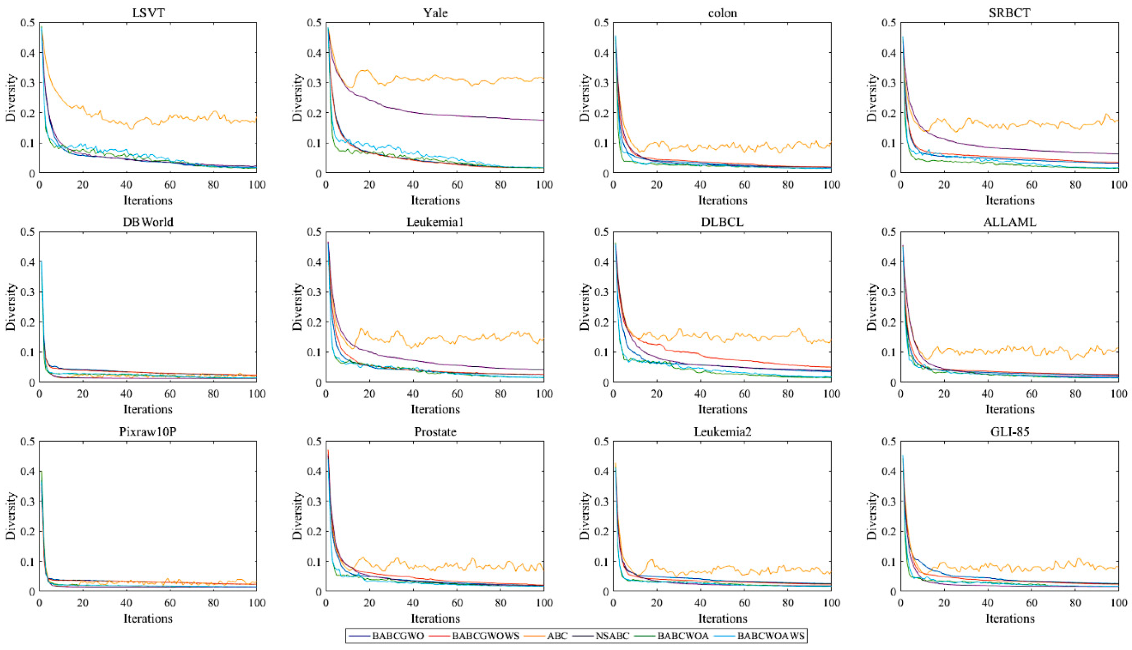
Figure 2 shows the diversity curves of six algorithms on 12 datasets. We can see that the diversity of ABC is obviously higher than that of other algorithms on all datasets, except DBWorld and Pixraw10P. According to the search process of the ABC algorithm, the exploration performance of the ABC algorithm is stronger, so its diversity is higher. In the early stage, high diversity can avoid trapping in the local optimization, but after a limited number of cycles, we need to find the optimal solution. The diversity of NSABC decreases a lot, which weakens the exploration ability of the ABC algorithm. After introducing the GWO and WOA operators into the framework, the diversity of these algorithms decreases faster than that of the NSABC algorithm in most datasets. The lower the diversity, the weaker the exploration ability of the algorithm and the stronger the exploitation ability of the algorithm. This shows that the introduction of the GWO and WOA operators strengthens the exploitation ability of the algorithm effectively. In addition, Figure 2 shows that the diversity curves of the BABCGWOWS algorithm and BABCGWO algorithm are similar, and the diversity curves of the BABCWOAWS algorithm and BABCWOA algorithm are not very different. It can be seen that scout bees have little effect on the diversity of the algorithms in this framework.

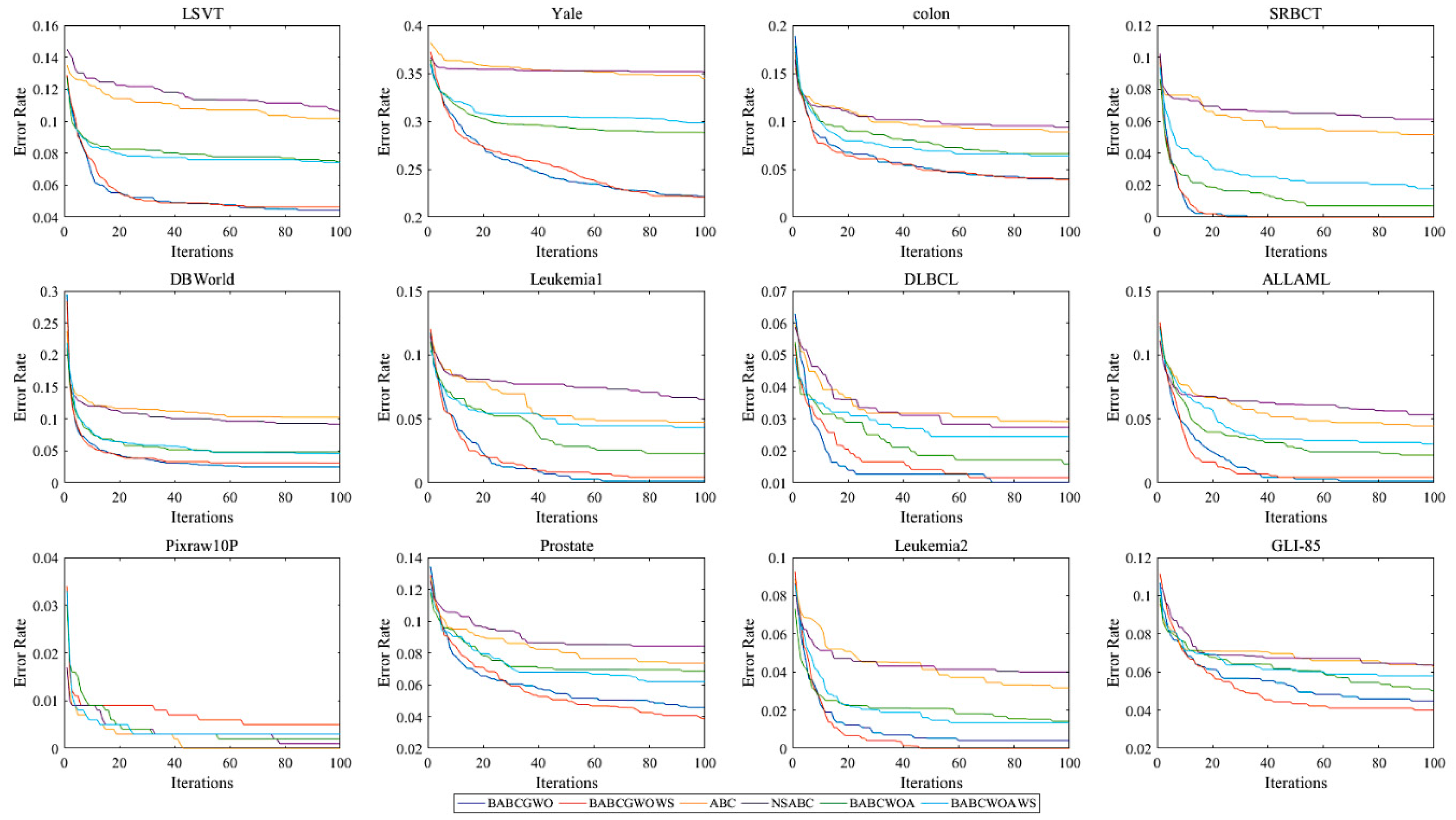
The convergence curves of the algorithms are plotted in Figure 3. This shows the decline of the error rate. Each curve is plotted by averaging the error rate obtained at each generation of the 10 runs. The convergence results of NSABC and ABC are similar on LSVT, Yale, colon, DBWorld, DLBCL, Pixraw10P and GLI_85 datasets, and the convergence results of the NSABC algorithm are slightly higher than that of the ABC algorithm on other datasets. Obviously, compared with the ABC algorithm, the BABCGWO and BABCWOA algorithms converge faster with a good-quality solution. On most datasets, the error rates of BABCGWO and BABCWOA are similar to or lower than those of BABCGWOWS and BABCWOAWS, respectively. It can be concluded that the BABCGWO and BABCWOA algorithms perform better than ABC in terms of both convergence speed and solution quality.

Table 2. Comparisons of error rate between different ABC-based methods.

Datasets	Index	Algorithms
		ABC	NSABC	BABCWOA	BABCWOAWS	BABCGWO	BABCGWOWS
LSVT	worst	0.112	0.121	0.103	0.104	0.056	0.064
	mean ± std	0.102 ± 0.01	0.106 ± 0.01	0.075 ± 0.02	0.074 ± 0.02	0.044 ± 0.01	0.046 ± 0.01
	best	0.087	0.089	0.047	0.047	0.031	0.031
Yale	worst	0.357	0.370	0.326	0.345	0.238	0.240
	mean ± std	0.345 ± 0.01	0.351 ± 0.01	0.288 ± 0.03	0.299 ± 0.04	0.220 ± 0.01	0.220 ± 0.01
	best	0.327	0.327	0.241	0.243	0.210	0.207
colon	worst	0.112	0.1	0.112	0.083	0.064	0.064
	mean ± std	0.089 ± 0.02	0.094 ± 0.01	0.066 ± 0.02	0.064 ± 0.02	0.037 ± 0.02	0.038 ± 0.02
	best	0.0643	0.081	0.05	0.048	0.014	0.014
SRBCT	worst	0.063	0.071	0.024	0.046	0.000	0.000
	mean ± std	0.052 ± 0.01	0.061 ± 0.01	0.007 ± 0.01	0.018 ± 0.02	0.000	0.000
	best	0.022	0.047	0.000	0.000	0.000	0.000
DBWorld	worst	0.121	0.110	0.093	0.074	0.033	0.048
	mean ± std	0.103 ± 0.01	0.092 ± 0.01	0.048 ± 0.02	0.046 ± 0.02	0.025 ± 0.01	0.031 ± 0.01
	best	0.088	0.079	0.017	0.029	0.014	0.014
Leukemia1	worst	0.068	0.086	0.043	0.071	0.014	0.029
	mean ± std	0.047 ± 0.02	0.065 ± 0.01	0.023 ± 0.02	0.043 ± 0.02	0.001 ± 0.01	0.004 ± 0.01
	best	0.027	0.039	0.000	0.014	0.000	0.000
DLBCL	worst	0.039	0.0518	0.041	0.041	0.025	0.038
	mean ± std	0.029 ± 0.01	0.027 ± 0.02	0.016 ± 0.01	0.025 ± 0.01	0.010 ± 0.01	0.012 ± 0.01
	best	0.025	0.000	0.000	0.000	0.000	0.000
ALLAML	worst	0.057	0.071	0.070	0.068	0.014	0.014
	mean ± std	0.045 ± 0.01	0.053 ± 0.01	0.022 ± 0.03	0.030 ± 0.03	0.001 ± 0.01	0.004 ± 0.01
	best	0.029	0.029	0.000	0.000	0.000	0.000
Pixraw10P	worst	0.000	0.010	0.010	0.010	0.010	0.010
	mean ± std	0.000	0.001 ± 0.00	0.002 ± 0	0.003 ± 0	0.003 ± 0.01	0.005 ± 0.01
	best	0.000	0.000	0.000	0.000	0.000	0.000
Prostate	worst	0.089	0.089	0.089	0.078	0.060	0.060
	mean ± std	0.074 ± 0.01	0.084 ± 0.00	0.069 ± 0.02	0.062 ± 0.01	0.044 ± 0.01	0.039 ± 0.01
	best	0.049	0.078	0.040	0.049	0.029	0.020
Leukemia2	worst	0.043	0.070	0.043	0.039	0.027	0.000
	mean ± std	0.032 ± 0.01	0.040 ± 0.01	0.014 ± 0.01	0.013 ± 0.01	0.004 ± 0.01	0.000
	best	0.014	0.013	0.000	0.000	0.000	0.000
GLI_85	worst	0.081	0.079	0.074	0.082	0.061	0.061
	mean ± std	0.062 ± 0.01	0.064 ± 0.01	0.050 ± 0.01	0.058 ± 0.02	0.045 ± 0.01	0.040 ± 0.01
	best	0.046	0.047	0.033	0.025	0.035	0.035

shows the worst, the best, the mean and the standard deviation of the error rate results of each algorithm. The ultimate goal of FS is to improve generalization performance, which means achieving a lower error rate when used on unforeseeable data. A lower error rate indicates that the algorithm can find a better feature subset. Since almost all the SI-based algorithms are stochastic in nature, they may produce different results in each run. Therefore, standard deviation is conducted to measure the variations in the results. The smaller the standard deviation is, the more stable the algorithm is.

From Table 2, we can see that the error rate of the NSABC algorithm is slightly higher than that of the ABC algorithm used on most datasets, but the increase is not more than 0.01. The error rate was improved on all datasets except Pixraw10P after the introduction of the operator with strong exploitation ability in the onlooker bee phase. Specifically, BABCWOA’s average error rate is at least 0.005 lower than the average error rate of the ABC algorithm, applied on the Prostate dataset. When used on the Yale dataset, the average error rate decreased the most, by nearly 0.06, and on the SRBCT and DBWorld datasets, the average error rate decreased by about 0.05. On other datasets, the average error rate also decreased by about 0.01 to 0.03. Moreover, the average error rate of BABCGWO was reduced more, especially on the Yale dataset, and BABCGWO decreased by 0.125 compared with the ABC algorithm. The average error rate of BABCGWO is at least 0.017 lower than that of the ABC algorithm when used on the GLI_85 dataset. There are seven datasets on which the average error rate decreased by more than 0.04. As you can see, the error rate of BABCGWOWS did not change much on most datasets compared to BABCGWO, and the results of comparison between BABCWOAWS and BABCWOA are similar.

In terms of the worst error rate, the BABCWOA algorithm was reduced on half of the datasets, while the BABCGWO algorithm improved on all datasets except Pixraw10P, and the maximum error rate decreased the most on the Yale dataset (by 0.119). Both BABCWOA and BABCGWO decreased in terms of the error rate. It can be seen from the standard deviation of the algorithm that although the error rate of the BABCWOA algorithm improved on the whole, its error rate was not as stable as the ABC algorithm’s on a few datasets, such as Yale and ALLAML. The stability of the BABCGWO algorithm is similar to that of the ABC algorithm. It can be concluded that the introduction of operators with strong exploitation ability into the proposed framework can indeed improve the ABC algorithm to a certain extent, and the scout bee phase is not active and has little effect on reducing the error rate of the algorithm.

As per the results in

Table 3. Comparisons of the number of selected features between different ABC-based methods.

Datasets	Index	Algorithms
		ABC	NSABC	BABCWOA	BABCWOAWS	BABCGWO	BABCGWOWS
LSVT	worst	20	15	167	157	65	64
	mean ± std	8.9 ± 4.58	6.8 ± 3.88	83.7 ± 50.61	104.5 ± 34.07	30.0 ± 16.83	33.4 ± 15.07
	best	4	3	27	61	15	16
Yale	worst	147	284	421	477	126	124
	mean ± std	96.9 ± 46.24	122.6 ± 88.40	245.6 ± 97.77	347.9 ± 103.06	102.4 ± 14.55	97.9 ± 21.37
	best	30	37	127	210	86	55
colon	worst	30	40	266	532	112	169
	mean ± std	18.5 ± 6.69	20.3 ± 8.53	142.8 ± 68.85	155.1 ± 138.18	80.4 ± 17.39	105.9 ± 28.05
	best	12	12	46	61	58	76
SRBCT	worst	584	104	497	829	233	353
	mean ± std	121.2 ± 166.69	64.8 ± 27.37	109.4 ± 254.02	394.5 ± 191.01	164.6 ± 45.35	204.0 ± 86.09
	best	25	21	112	151	107	116
DBWorld	worst	44	40	484	423	297	263
	mean ± std	32.3 ± 5.25	31.7 ± 5.08	249.4 ± 112.93	317.7 ± 99.99	216.2 ± 59.40	205.6 ± 52.63
	best	23	22	92	154	109	119
Leukemia1	worst	147	676	1694	1247	692	410
	mean ± std	71.6 ± 30.28	149 ± 210.69	648.2 ± 504.44	741.6 ± 324.58	277.4 ± 156.79	300.5 ± 73.80
	best	42	30	237	305	160	182
DLBCL	worst	128	695	1029	1484	1427	1413
	mean ± std	59.4 ± 30.28	126.1 ± 202.79	545.3 ± 314.94	811.6 ± 532.06	458.4 ± 358.90	684.7 ± 464.70
	best	32	28	230	143	228	190
ALLAML	worst	97	82	646	1168	370	444
	mean ± std	66.5 ± 19.17	50.9 ± 11.54	386.4 ± 144.24	500.4 ± 286.34	276.4 ± 54.91	305.7 ± 87.46
	best	45	42	168	217	198	156
Pixraw10P	worst	115	88	294	370	405	349
	mean ± std	73.7 ± 17.81	66.8 ± 8.34	196.1 ± 56.32	200.4 ± 74.22	218.5 ± 76.059	253.5 ± 63.50
	best	52	58	137	121	157	159
Prostate	worst	146	103	1454	1505	624	897
	mean ± std	91.3 ± 32.66	76.9 ± 15.57	1055.4 ± 362.08	797.8 ± 314.48	444.5 ± 129.06	569.6 ± 227.40
	best	56	55	442	445	199	250
Leukemia2	worst	295	124	1300	1246	1036	844
	mean ± std	115.8 ± 66.71	88.9 ± 18.75	876.4 ± 303.41	661.4 ± 273.88	582.6 ± 234.36	425.7 ± 153.55
	best	68	70	318	329	357	311
GLI_85	worst	248	173	5716	6691	2920	1453
	mean ± std	161.8 ± 32.20	150.1 ± 12.05	1576.3 ± 1508.28	1553.6 ± 1840.90	1204.4 ± 674.09	1099.2 ± 272.00
	best	138	131	437	520	697	681

, the number of features of the improved algorithm is more than that of the ABC algorithm. Although dimensionality reduction is one of the targets of FS, it is more important to achieve a lower error rate in many practical applications. Although the ABC algorithm has a small feature subset, it can be observed from the error rate in Table 2 that such a low number of selected features cannot achieve a low error rate.

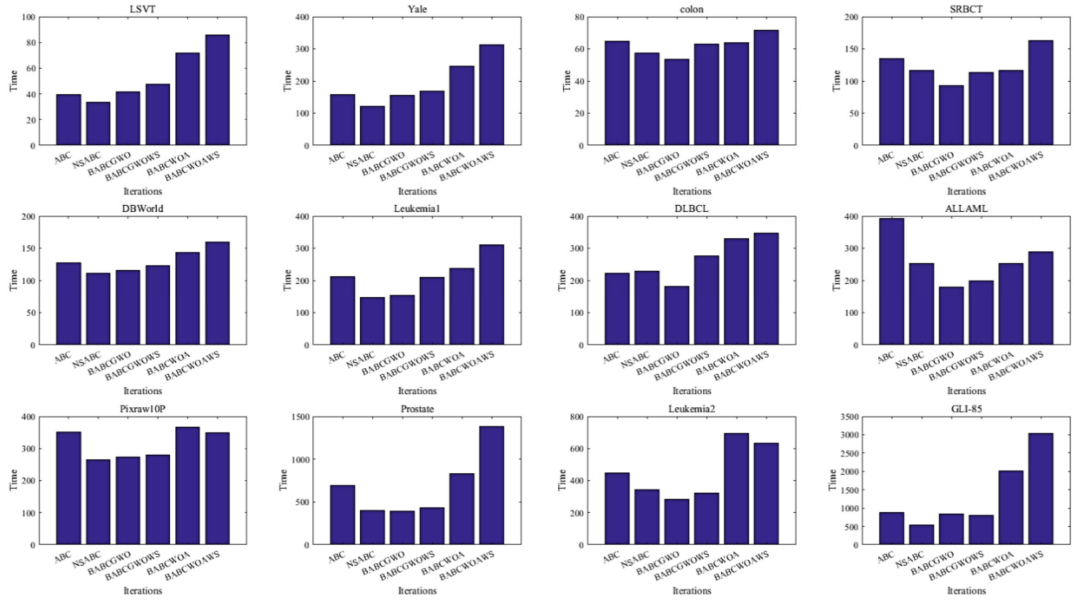
According to Figure 4, it is obvious that the calculation time will be reduced when the scout bee phase is removed. After the introduction of the GWO operator, the BABCGWO algorithm displayed little difference in time compared with the ABC or NSABC algorithms used on some datasets. In addition, BABCGWO was much faster than the ABC algorithm on colon, SRBCT, Leukemia1, DLBCL, ALLAML, Pixraw10P, Prostate, and Leukemia2 datasets. After the introduction of the WOA operator, the running time of the BABCWOA algorithm increased more or less on all datasets, except SRBCT and ALLAML, which may be because the running speed is also proportional to the feature number. It can be observed from Table 3 that the BABCWOA algorithm selects more features than other algorithms.

To sum up, the proposed framework can effectively make the convergence speed faster, reduce the diversity, and find a better optimal solution. Although the number of features increases, the classification error rate of the algorithm decreases significantly after introducing an operator with strong exploitation ability into the framework. The scout bee phase has very little effect on improving the fitness value of the solution and consumes computational resources and memory, so the scout bee phase is omitted in this framework. From the above analysis, we can conclude that using the proposed framework can effectively improve the performance of the ABC algorithm.

6. Further Analysis

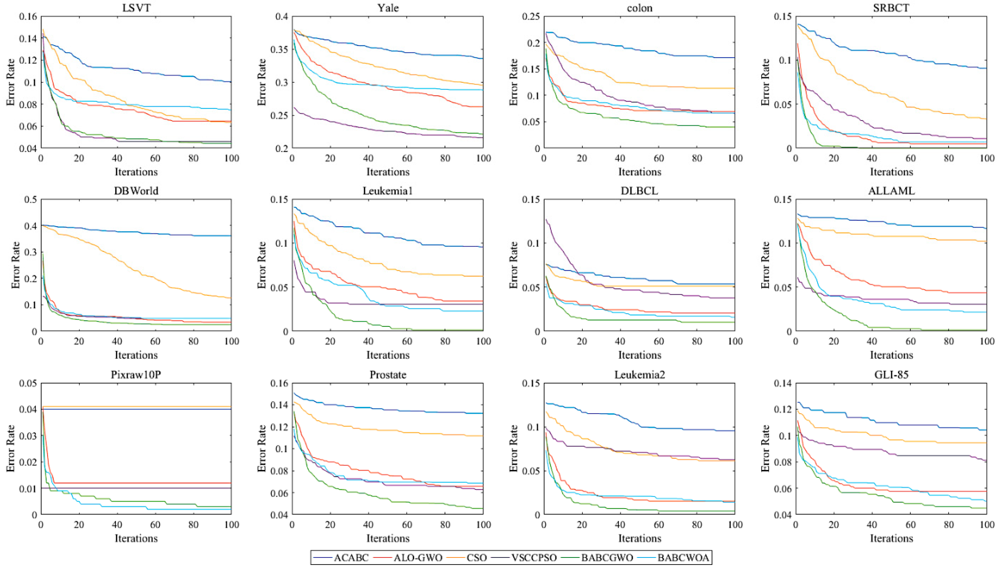
The comparisons in Section 5 show that the proposed BABCGWO algorithm and BABCWOA algorithm are more efficient than the ABC algorithm. To make a complete evaluation, we further verify the effectiveness of BABCGWO algorithm and BABCWOA algorithm by comparing them with four state-of-the-art FS algorithms on high-dimensional datasets, including the popular PSO variants named CSO [40] and VSCCPSO [41], the novel GWO variant ALO_GWO [42], and an ABC variant named ACABC [31]. In particular, CSO, VSCCPSO and ALO_GWO achieved excellent results in dealing with high-dimensional datasets. The parameters applied in CSO, VSCCPSO, ALO_GWO and ACABC here are the same as their own parameter settings.

In this section, the classification error rate, the size of the feature subset, the computational time and the convergence curve of the six algorithms are investigated. The best results are shown in bold in the table. To further verify the improved effect of the two algorithms proposed in this paper, the Wilcoxon’s rank sum test [43,44] with a significance level of 0.05 is applied to test the statistical significance between two different algorithms. The error rate, number of features and execution time of the two algorithms are tested by Wilcoxon rank sum test with another four FS algorithms. In the table of Wilcoxon rank sum test, the symbol “+” indicates that the proposed algorithms are significantly better than the compared algorithm, the symbol “=” means that the performance of the two algorithms is similar, and the symbol “−” is opposite to “+”, indicating that the proposed algorithms are significantly worse than other algorithms.

Table 4. Comparison of error rates of algorithms.

Datasets	Index	Algorithms
		CSO	VSCCPSO	ALO_GWO	ACABC	BABCWOA	BABCGWO
LSVT	worst	0.081	0.064	0.078	0.080	0.075	0.056
	mean ± std	0.063 ± 0.01	0.046 ± 0.01	0.065 ± 0.04	0.065 ± 0.01	0.075 ± 0.02	0.044 ± 0.01
	best	0.055	0.024	0.054	0.056	0.047	0.031
Yale	worst	0.320	0.230	0.309	0.315	0.326	0.238
	mean ± std	0.295 ± 0.02	0.216 ± 0.01	0.273 ± 0.02	0.288 ± 0.02	0.288 ± 0.03	0.220 ± 0.01
	best	0.268	0.200	0.254	0.266	0.241	0.210
colon	worst	0.176	0.081	0.088	0.157	0.112	0.064
	mean ± std	0.113 ± 0.03	0.065 ± 0.01	0.069 ± 0.01	0.119 ± 0.02	0.066 ± 0.02	0.037 ± 0.02
	best	0.081	0.048	0.064	0.095	0.050	0.014
SRBCT	worst	0.049	0.024	0.025	0.063	0.024	0.000
	mean ± std	0.033 ± 0.02	0.011 ± 0.01	0.005 ± 0.01	0.035 ± 0.01	0.007 ± 0.01	0.000
	best	0.000	0.000	0.000	0.022	0.000	0.000
DBWorld	worst	0.255	0.091	0.062	0.198	0.093	0.033
	mean ± std	0.126 ± 0.05	0.048 ± 0.01	0.034 ± 0.01	0.139 ± 0.03	0.048 ± 0.02	0.025 ± 0.01
	best	0.062	0.026	0.017	0.093	0.017	0.014
Leukemia1	worst	0.084	0.056	0.057	0.07	0.043	0.014
	mean ± std	0.062 ± 0.01	0.031 ± 0.01	0.034 ± 0.02	0.058 ± 0.01	0.023 ± 0.02	0.001 ± 0.01
	best	0.039	0.028	0.000	0.041	0.000	0.000
DLBCL	worst	0.075	0.091	0.038	0.064	0.041	0.025
	mean ± std	0.051 ± 0.01	0.038 ± 0.02	0.021 ± 0.01	0.038 ± 0.02	0.016 ± 0.01	0.010 ± 0.01
	best	0.038	0.026	0.000	0.013	0.000	0.000
ALLAML	worst	0.113	0.056	0.082	0.121	0.070	0.014
	mean ± std	0.102 ± 0.01	0.031 ± 0.01	0.044 ± 0.03	0.103 ± 0.01	0.022 ± 0.03	0.001 ± 0.01
	best	0.093	0.014	0.000	0.082	0.000	0.000
Pixraw10P	worst	0.050	0.010	0.040	0.040	0.010	0.010
	mean ± std	0.041 ± 0.00	0.010	0.012 ± 0.01	0.040	0.002 ± 0	0.003 ± 0.01
	best	0.040	0.010	0.000	0.040	0.000	0.000
Prostate	worst	0.126	0.078	0.079	0.117	0.089	0.060
	mean ± std	0.112 ± 0.01	0.063 ± 0.01	0.066 ± 0.01	0.106 ± 0.01	0.069 ± 0.02	0.044 ± 0.01
	best	0.089	0.049	0.049	0.087	0.040	0.029
Leukemia2	worst	0.082	0.097	0.029	0.095	0.043	0.027
	mean ± std	0.061 ± 0.01	0.063 ± 0.02	0.015 ± 0.01	0.054 ± 0.02	0.014 ± 0.01	0.004 ± 0.01
	best	0.041	0.028	0.000	0.027	0.000	0.000
GLI_85	worst	0.129	0.106	0.071	0.150	0.074	0.061
	mean ± std	0.094 ± 0.02	0.074 ± 0.02	0.058 ± 0.01	0.109 ± 0.02	0.050 ± 0.01	0.045 ± 0.01
	best	0.081	0.047	0.047	0.082	0.033	0.035

shows the worst, best, average, and standard deviation of the error rate for each algorithm. In terms of the maximum error rate and average error rate, the BABCGWO algorithm performed worse than any other algorithms in all datasets except Yale and Pixraw10P, and it was reduced by several percentage points on most datasets. The BABCWOA algorithm outperformed the four compared algorithms on half of the datasets, and achieved the best average error rate of all algorithms on the Pixraw10P dataset. In terms of minimum error rate, the BABCGWO algorithm’s was lower than the other algorithms when applied all datasets except LVST, Yale and GLI_85. The BABCWOA algorithm also outperformed the four algorithms on more than half of the datasets. The standard deviation of the BABCGWO algorithm was ≤0.01 on most datasets and 0.02 on the colon dataset only, which is significantly superior to most other algorithms, indicating that the BABCGWO algorithm has better stability compared with the other algorithms. However, the standard deviation of the BABCWOA algorithm is mostly about 0.02, which is not much different from the four compared algorithms.

To further illustrate whether the error rates of the algorithms proposed in this paper are significantly different from those of other algorithms, we use the Wilcoxon rank sum test. As can be seen from the Wilcoxon rank sum test results of the error rate in

Table 5. Wilcoxon rank sum test on error rates of algorithms.

Datasets	CSO		VSCCPSO		ALO_GWO		ACABC
	BABCGWO	BABCWOA	BABCGWO	BABCWOA	BABCGWO	BABCWOA	BABCGWO	BABCWOA
LSVT	0(+)	0.04(−)	0.68(=)	0(−)	0(+)	0.08(=)	0(+)	0.10(=)
Yale	0(+)	0.57(=)	0.52(=)	0(−)	0(+)	0.20(=)	0(+)	0.97(=)
colon	0(+)	0(+)	0(+)	0.47(=)	0(+)	0.09(=)	0(+)	0(+)
SRBCT	0(+)	0(+)	0(+)	0.55(=)	0.08(=)	0.62(=)	0(+)	0(+)
DBWorld	0(+)	0(+)	0(+)	0.84(=)	0.06(=)	0.11(=)	0(+)	0(+)
Leukemia1	0(+)	0(+)	0(+)	0.72(=)	0(+)	0.17(=)	0(+)	0(+)
DLBCL	0(+)	0(+)	0(+)	0.01(+)	0(+)	0.44(=)	0(+)	0.01(+)
ALLAML	0(+)	0(+)	0(+)	0.16(=)	0(+)	0.05(=)	0(+)	0(+)
Pixraw10P	0(+)	0(+)	0.10(=)	0.01(+)	0.01(+)	0(+)	0(+)	0(+)
Prostate	0(+)	0(+)	0(+)	0.38(=)	0(+)	0.73(=)	0(+)	0(+)
Leukemia2	0(+)	0(+)	0(+)	0(+)	0.02(+)	0.82(=)	0(+)	0(+)
GLI_85	0(+)	0(+)	0(+)	0(+)	0(+)	0.10(=)	0(+)	0(+)

, compared with the ACABC and CSO algorithms, the error rates of the algorithms proposed in this paper were almost significantly lower than those of the other four algorithms when used on 12 datasets. Compared with the VSCCPSO algorithm, the BABCGWO algorithm was superior to the VSCCPSO algorithm when used on all datasets except LSVT, Yale and Pixraw10P. The BABCWOA algorithm was also significantly improved compared with the VSCCPSO algorithm when used on some datasets, and there was little difference in the error rate between BABCWOA and VSCCPSO for most datasets. Compared with the ALO_GWO algorithm, the error rate of the BABCGWO algorithm was significantly lower than that of the ALO_GWO algorithm for all datasets except SRBCT and DBWorld, and there was almost no notable difference between the BABCWOA and ALO_GWO algorithms.

The experimental results in

Table 6. Comparison of the average numbers of selected features and average execution times of algorithms.

Datasets	Index	Algorithms
		CSO	VSCCPSO	ALO_GWO	ACABC	BABCWOA	BABCGWO
LSVT	Subsets	151.5	37.5	102.5	150.9	83.7	30.0
	Time	55.5	83.4	89.6	172.1	71.7	41.9
Yale	Subsets	504.1	150.1	240.6	506.3	245.6	102.4
	Time	147.2	482.0	291.2	464.6	245.6	156.0
colon	Subsets	983.0	194.0	261.2	995.6	142.8	80.4
	Time	55.8	153.4	287.6	271.7	63.8	53.4
SRBCT	Subsets	1127.1	205.8	408.3	1136.2	109.4	164.6
	Time	101.5	275.0	311.0	381.8	116.9	93.2
DBWorld	Subsets	2316.2	601.4	446.5	2338.0	249.4	216.2
	Time	268.7	419.9	841.0	901.8	144.1	115.5
Leukemia1	Subsets	2664.6	721.2	867.4	2645.6	648.2	277.4
	Time	417.7	549.0	774.6	1257.0	238.1	153.9
DLBCL	Subsets	2737.6	625.6	1097.8	2733.1	545.3	458.4
	Time	436.2	631.8	1259.8	2409.6	330.4	182.1
ALLAML	Subsets	3563.3	1248.9	846.5	3537.0	386.4	276.4
	Time	646.2	828.0	780.6	2954.4	252.0	180.3
Pixraw10P	Subsets	5015.6	2366.7	882.1	5006.7	196.1	218.5
	Time	1647.9	3417.9	1428.1	4187.3	367.0	253.3
Prostate	Subsets	5246.2	1558.7	1440.3	5194.9	1055.4	444.5
	Time	1418.7	2261.7	2435.9	8370.3	829.8	391.0
Leukemia2	Subsets	5627.1	2091.2	1336.5	5608.7	876.4	582.6
	Time	852.6	1820.4	2342.9	2722.6	693.8	282.9
GLI_85	Subsets	11,157.5	5167.9	2971.2	11,682.5	1576.3	1204.4
	Time	3996.3	3872.9	3013.8	9230.0	2023.4	836.3

show the average number of selected features and average execution time of the six algorithms across 10 runs on 12 datasets. One of the purposes of FS is to remove redundant and irrelevant features so as to strengthen the classification performance of the algorithm. In the case of the same error rate, the smaller number of selected features indicates that the algorithm can find a better feature subset. The experimental results show that the average number of features selected by the BABCGWO algorithm is less than that of other algorithms for 12 datasets, its running time is shorter than that of other algorithms in all datasets except Yale, and its running speed is only slower than that of the CSO algorithm for the Yale dataset. The BABCWOA algorithm selects fewer features than the four compared algorithms on all datasets except LSVT and Yale, and the BABCWOA algorithm runs faster than the compared algorithms on 8 of the 12 datasets, and is second only to the CSO algorithm on the remaining 4 datasets. Therefore, although the error rate of the BABCWOA algorithm is not significantly improved on some datasets, it does improve the size of feature subsets and running time. This indicates that, compared with other algorithms, the algorithms proposed in this paper can find a feature subset with smaller size in a shorter time, and achieve a lower error rate.

The Wilcoxon rank sum test results in

Table 7. Wilcoxon rank sum test on the numbers of features selected by algorithms.

Datasets	CSO		VSCCPSO		ALO_GWO		ACABC
	BABCGWO	BABCWOA	BABCGWO	BABCWOA	BABCGWO	BABCWOA	BABCGWO	BABCWOA
LSVT	0(+)	0(+)	0.10(=)	0.03(−)	0(+)	0.33(=)	0(+)	0(+)
Yale	0(+)	0(+)	0(+)	0.57(=)	0(+)	0.05(=)	0(+)	0(+)
colon	0(+)	0(+)	0(+)	0.03(+)	0(+)	0.02(+)	0(+)	0(+)
SRBCT	0(+)	0(+)	0.04(+)	0.16(=)	0(+)	0.01(+)	0(+)	0(+)
DBWorld	0(+)	0(+)	0(+)	0(+)	0(+)	0.01(+)	0(+)	0(+)
Leukemia1	0(+)	0(+)	0(+)	0.05(=)	0(+)	0.04(+)	0(+)	0(+)
DLBCL	0(+)	0(+)	0.01(+)	0.34	0(+)	0.01(+)	0(+)	0(+)
ALLAML	0(+)	0(+)	0(+)	0(+)	0(+)	0(+)	0(+)	0(+)
Pixraw10P	0(+)	0(+)	0(+)	0(+)	0.03(+)	0.02(+)	0(+)	0(+)
Prostate	0(+)	0(+)	0(+)	0(+)	0(+)	0.19(=)	0(+)	0(+)
Leukemia2	0(+)	0(+)	0(+)	0(+)	0(+)	0(+)	0(+)	0(+)
GLI_85	0(+)	0(+)	0(+)	0(+)	0(+)	0(+)	0(+)	0(+)

show that the feature subsets selected by the algorithms proposed in this paper are significantly smaller than those of the ACABC and CSO algorithms applied on the 12 datasets. Compared with ALO_GWO and VSCCPSO, the feature numbers of the proposed algorithms are not significantly lower than those of the two algorithms, but for only a few datasets.

As can be seen from the results in

Table 8. Wilcoxon rank sum test on the execution times of algorithms.

Datasets	CSO		VSCCPSO		ALO_GWO		ACABC
	BABCGWO	BABCWOA	BABCGWO	BABCWOA	BABCGWO	BABCWOA	BABCGWO	BABCWOA
LSVT	0(+)	0.91(=)	0(+)	0.43(=)	0(+)	0.24(=)	0(+)	0(+)
Yale	0.19(=)	0(−)	0(+)	0(+)	0(+)	0.03(+)	0(+)	0(+)
colon	0(+)	0.06(=)	0(+)	0(+)	0(+)	0(+)	0(+)	0(+)
SRBCT	0.12(=)	0.03(−)	0(+)	0(+)	0(+)	0(+)	0(+)	0(+)
DBWorld	0(+)	0(+)	0(+)	0(+)	0(+)	0(+)	0(+)	0(+)
Leukemia1	0(+)	0(+)	0(+)	0(+)	0(+)	0(+)	0(+)	0(+)
DLBCL	0(+)	0.03(+)	0(+)	0(+)	0(+)	0(+)	0(+)	0(+)
ALLAML	0(+)	0(+)	0(+)	0(+)	0(+)	0(+)	0(+)	0(+)
Pixraw10P	0(+)	0(+)	0(+)	0(+)	0(+)	0(+)	0(+)	0(+)
Prostate	0(+)	0(+)	0(+)	0(+)	0(+)	0(+)	0(+)	0(+)
Leukemia2	0(+)	0.14(=)	0(+)	0(+)	0(+)	0(+)	0(+)	0(+)
GLI_85	0(+)	0(+)	0(+)	0(+)	0(+)	0(+)	0(+)	0(+)

, the proposed algorithms are not much different from, or are slower than, the other algorithms for only a few datasets. On most datasets, the two algorithms are significantly faster than other algorithms.

The convergence curves of the algorithms for 12 datasets are shown in Figure 5. These curves confirm that the BABCGWO algorithm converges more rapidly, with a good quality of solution, than other algorithms in the first 20 iterations, which indicates that the optimization precision and optimization speed of BABCGWO algorithm are better than those of other algorithms. The BABCWOA algorithm also has a faster convergence curve on most datasets, and can obtain a lower error rate.

In conclusion, the proposed framework is effective. The exploration ability of the ABC algorithm is successfully combined with the updating mode of the algorithm with a strong exploitation ability, such that the BABCGWO algorithm and BABCWOA algorithm can find optimal solutions with lower error rates and fewer feature numbers in a shorter period of time.

7. Conclusions

There are often redundant and irrelevant features in high-dimensional datasets, so the FS method is used for data preprocessing. Aiming at the strong exploration ability of the ABC algorithm, this study proposes a framework that integrates the updating operators of the algorithm with strong exploitation abilities into the ABC algorithm to make the exploration and exploitation abilities balanced. Moreover, since the removal of the scout bee phase can weaken the exploration ability and save computational resources when processing high-dimensional datasets, the scout bee phase in the ABC algorithm is left out in our framework, and thus the BABCGWO algorithm and BABCWOA algorithm are proposed to deal with the FS problem in high-dimensional datasets. The experimental results show that on 12 high-dimensional datasets, the BABCGWO algorithm and BABCWOA algorithm are significantly superior to other algorithms as regards dimensionality reduction, classification error rate and execution time. This shows that the proposed framework can balance the capabilities of exploration and exploitation, and effectively improve the overall performance in FS.

However, the proposed method mainly focuses on the single-objective feature selection problem, where the main aim is to reduce the algorithm’s classification error rate. In the future, we will investigate a multi-objective FS algorithm that simultaneously maximizes the classification performance and minimizes the number of selected features. Moreover, we would like to employ algorithms in different domains to verify their universality.

References

- Dash, M.; Liu, H. Feature selection for classification. Intell. Data Anal. 1997, 1, 131–156. [Google Scholar] [CrossRef]
- Guyon, I.; Elisseeff, A. An introduction to variable and feature selection. J. Mach. Learn. Res. 2003, 3, 1157–1182. [Google Scholar]
- Mafarja, M.M.; Mirjalili, S. Hybrid Whale Optimization Algorithm with simulated annealing for feature selection. Neurocomputing 2017, 260, 302–312. [Google Scholar] [CrossRef]
- Gao, W.F.; Liu, S.Y.; Huang, L.L. A global best artificial bee colony algorithm for global optimization. J. Comput. Appl. Math. 2012, 236, 2741–2753. [Google Scholar] [CrossRef] [Green Version]
- Poli, R.; Kennedy, J.; Blackwell, T. Particle swarm optimization. Swarm Intell. 2007, 1, 33–57. [Google Scholar] [CrossRef]
- Wang, Y.; Cai, Z.; Zhang, Q. Differential evolution with composite trial vector generation strategies and control parameters. IEEE Trans. Evol. Comput. 2011, 15, 55–66. [Google Scholar] [CrossRef]
- Mirjalili, S.; Mirjalili, S.M.; Lewis, A. Grey Wolf Optimizer. Adv. Eng. Softw. 2014, 69, 46–61. [Google Scholar] [CrossRef] [Green Version]
- Mirjalili, S.; Lewis, A. The whale optimization algorithm. Adv. Eng. Softw. 2016, 95, 51–67. [Google Scholar] [CrossRef]
- Xue, B.; Zhang, M.; Browne, W.N.; Yao, X. A survey on evolutionary computation approaches to feature selection. IEEE Trans. Evol. Comput. 2015, 20, 606–626. [Google Scholar] [CrossRef] [Green Version]
- Djellali, H.; Djebbar, A.; Zine, N.G.; Azizi, N. Hybrid artificial bees colony and particle swarm on feature selection. In Proceedings of the International Conference on Computational Intelligence and Its Applications, Oran, Algeria, 8–10 May 2018; Springer: Cham, Switzerland, 2018; pp. 93–105. [Google Scholar]
- Zorarpacı, E.; Özel, S.A. A hybrid approach of differential evolution and artificial bee colony for feature selection. Expert Syst. Appl. 2016, 62, 91–103. [Google Scholar] [CrossRef]
- Al-Tashi, Q.; Kadir, S.J.A.; Rais, H.M.; Mirjalili, S.H. Alhussian, Binary Optimization Using Hybrid Grey Wolf Optimization for Feature Selection. IEEE Access 2019, 7, 39496–39508. [Google Scholar] [CrossRef]
- Shi, Y.; Pun, C.M.; Hu, H.; Gao, H. An improved artificial bee colony and its application. Knowl. Based Syst. 2016, 107, 14–31. [Google Scholar] [CrossRef]
- Garg, D.P.; Kumar, M. Optimization techniques applied to multiple manipulators for path planning and torque minimization. Eng. Appl. Artif. Intell. 2002, 15, 241–252. [Google Scholar] [CrossRef] [Green Version]
- Roberge, V.; Tarbouchi, M.; Labonté, G. Comparison of parallel genetic algorithm and particle swarm optimization for real-time UAV path planning. IEEE Trans. Ind. Inform. 2012, 9, 132–141. [Google Scholar] [CrossRef]
- Zhang, Y.; Gong, D.-W.; Zhang, J.-H. Robot path planning in uncertain environment using multi-objective particle swarm optimization. Neurocomputing 2013, 103, 172–185. [Google Scholar] [CrossRef]
- Oh, I.-S.; Lee, J.-S.; Moon, B.-R. Hybrid genetic algorithms for feature selection. IEEE Trans. Pattern Anal. Mach. Intell. 2004, 26, 1424–1437. [Google Scholar]
- Palanisamy, S.; Kanmani, S. Artificial bee colony approach for optimizing feature selection. Int. J. Comput. Sci. Issues 2012, 9, 432. [Google Scholar]
- Tran, B.; Xue, B.; Zhang, M. Improved PSO for feature selection on high-dimensional datasets. In Proceedings of the Asia-Pacific Conference on Simulated Evolution and Learning, Dunedin, New Zealand, 15–18 December 2014; Springer: Cham, Switzerland, 2014; pp. 503–515. [Google Scholar]
- Liang, Y.; Leung, K.-S. Genetic algorithm with adaptive elitist-population strategies for multimodal function optimization. Appl. Soft Comput. 2011, 11, 2017–2034. [Google Scholar] [CrossRef]
- Mirjalili, S.; Hashim, S.Z.M. A new hybrid PSOGSA algorithm for function optimization. In Proceedings of the 2010 International Conference on Computer and Information Application, Tianjin, China, 3–5 December 2010; IEEE: Piscataway, NJ, USA, 2010; pp. 374–377. [Google Scholar]
- Pan, Q.-K.; Sang, H.-Y.; Duan, J.-H.; Gao, L. An improved fruit fly optimization algorithm for continuous function optimization problems. Knowl. Based Syst. 2014, 62, 69–83. [Google Scholar] [CrossRef]
- Clerc, M. Discrete particle swarm optimization, illustrated by the traveling salesman problem. In New Optimization Techniques in Engineering; Springer: Berlin/Heidelberg, Germany, 2004; pp. 219–239. [Google Scholar]
- Kan, J.M.; Zhang, Y. Application of an improved ant colony optimization on generalized traveling salesman problem. Energy Procedia 2012, 17, 319–325. [Google Scholar]
- Mahi, M.; Baykan, Ö.K.; Kodaz, H. A new hybrid method based on particle swarm optimization, ant colony optimization and 3-opt algorithms for traveling salesman problem. Appl. Soft Comput. 2015, 30, 484–490. [Google Scholar] [CrossRef]
- Li, A.-D.; Xue, B.; Zhang, M. Improved binary particle swarm optimization for feature selection with new initialization and search space reduction strategies. Appl. Soft Comput. 2021, 106, 107302. [Google Scholar] [CrossRef]
- Gao, W.F.; Liu, S.Y.; Jiang, F. An improved artificial bee colony algorithm for directing orbits of chaotic systems. Appl. Math. Comput. 2011, 218, 3868–3879. [Google Scholar] [CrossRef]
- Hancer, E.; Xue, B.; Karaboga, D.; Zhang, M. A binary ABC algorithm based on advanced similarity scheme for feature selection. Appl. Soft Comput. 2015, 36, 334–348. [Google Scholar] [CrossRef]
- Gaidhane, P.J.; Nigam, M.J. A hybrid grey wolf optimizer and artificial bee colony algorithm for enhancing the performance of complex systems. J. Comput. Sci. 2018, 27, 284–302. [Google Scholar] [CrossRef]
- Chao, X.Q.; Li, W. Feature selection method optimized by artificial bee colony algorithm. J. Front. Comput. Sci. Technol. 2019, 13, 300–309. [Google Scholar]
- Shunmugapriya, P.; Kanmani, S. A hybrid algorithm using ant and bee colony optimization for feature selection and classification (AC-ABC Hybrid). Swarm Evol. Comput. 2017, 36, 27–36. [Google Scholar] [CrossRef]
- Shunmugapriya, P.; Kanmani, S.; Supraja, R.; Saranya, K. Feature selection optimization through enhanced Artificial Bee Colony algorithm. In Proceedings of the 2013 International Conference on Recent Trends in Information Technology (ICRTIT), Chennai, India, 25–27 July 2013; IEEE: Piscataway, NJ, USA, 2013; pp. 56–61. [Google Scholar]
- Zhu, G.; Kwong, S. Gbest-guided artificial bee colony algorithm for numerical function optimization. Appl. Math. Comput. 2010, 217, 3166–3173. [Google Scholar] [CrossRef]
- Singh, A.; Deep, K. Exploration–exploitation balance in Artificial Bee Colony algorithm: A critical analysis. Soft Comput. 2019, 23, 9525–9536. [Google Scholar] [CrossRef]
- Hong, P.N.; Ahn, C.W. Fast artificial bee colony and its application to stereo correspondence. Expert Syst. Appl. 2016, 45, 460–470. [Google Scholar] [CrossRef]
- Emary, E.; Zawba, H.M.; Hassanien, A.E. Binary grey wolf optimization approaches for feature selection. Neurocomputing 2016, 172, 371–381. [Google Scholar] [CrossRef]
- Tu, Q.; Chen, X.C.; Liu, X.C. Multi-strategy ensemble grey wolf optimizer and its application to feature selection. Appl. Soft Comput. 2019, 76, 16–30. [Google Scholar] [CrossRef]
- Long, W.; Jiao, J.J.; Liang, X.M.; Tang, M.Z. An exploration-enhanced grey wolf optimizer to solve high-dimensional numerical optimization. Eng. Appl. Artif. Intell. 2018, 68, 63–80. [Google Scholar] [CrossRef]
- Liao, Y.; Vemuri, V.R. Use of K-Nearest Neighbor classifier for intrusion detection. Comput. Secur. 2002, 21, 439–448. [Google Scholar] [CrossRef]
- Gu, S.K.; Cheng, R.; Jin, Y.C. Feature selection for high-dimensional classification using a competitive swarm optimizer. Soft Comput. 2018, 22, 811–822. [Google Scholar] [CrossRef] [Green Version]
- Song, X.-F.; Zhang, Y.; Guo, Y.-N.; Sun, X.-Y.; Wang, Y.-L. Variable-Size Cooperative Coevolutionary Particle Swarm Optimization for Feature Selection on High-Dimensional Data. IEEE Trans. Evol. Comput. 2020, 24, 882–895. [Google Scholar] [CrossRef]
- Zawbaa, H.M.; Emary, E.; Grosan, C.; Snasel, V. Large-dimensionality small-instance set feature selection: A hybrid bio-inspired heuristic approach. Swarm Evol. Comput. 2018, 42, 29–42. [Google Scholar] [CrossRef]
- El-Kenawy, E.M.; Eid, M.M.; Saber, M.; Ibrahim, A. MbGWO-SFS: Modified Binary Grey Wolf Optimizer Based on Stochastic Fractal Search for Feature Selection. IEEE Access 2020, 8, 107635–107649. [Google Scholar] [CrossRef]
- Wilcoxon, F. Individual comparisons by ranking methods. In Breakthroughs in Statistics; Springer: New York, NY, USA, 1992; pp. 196–202. [Google Scholar]
Figure 1.
The flowchart of the ABC algorithm and our proposed framework.
Figure 2.
The diversity curves between different ABC-based methods.
Figure 3.
The convergence curves between different ABC-based methods.
Figure 4.
The execution time between different ABC-based methods.
Figure 5.
The convergence curves of algorithms.