Article

Parallel Implementation of the Algorithm to Compute Forest Fire Impact on Infrastructure Facilities of JSC Russian Railways

by
Nikolay Viktorovich Baranovskiy
1,2,*,
Aleksey Podorovskiy
2 and
Aleksey Malinin
1,2
1
School of Energy and Power Engineering, Tomsk Polytechnic University, 634050 Tomsk, Russia
2
Scientific Centre of Information Technologies and Artificial Intelligence, Sirius University of Science and Technology, 354340 Sochi, Russia
*
Author to whom correspondence should be addressed.
Submission received: 29 September 2021 / Revised: 8 November 2021 / Accepted: 12 November 2021 / Published: 15 November 2021
(This article belongs to the Collection Parallel and Distributed Computing: Algorithms and Applications)

Abstract

:
Forest fires have a negative impact on the economy in a number of regions, especially in Wildland Urban Interface (WUI) areas. An important link in the fight against fires in WUI areas is the development of information and computer systems for predicting the fire safety of infrastructural facilities of Russian Railways. In this work, a numerical study of heat transfer processes in the enclosing structure of a wooden building near the forest fire front was carried out using the technology of parallel computing. The novelty of the development is explained by the creation of its own program code, which is planned to be put into operation either in the Information System for Remote Monitoring of Forest Fires ISDM-Rosleskhoz, or in the information and computing system of JSC Russian Railways. In the Russian Federation, it is forbidden to use foreign systems in the security services of industrial facilities. The implementation of the deterministic model of heat transfer in the enclosing structure with the complexity of the algorithm O (2N2 + 2K) is presented. The program is implemented in Python 3.x using the NumPy and Concurrent libraries. Calculations were carried out on a multiprocessor cluster in the Sirius University of Science and Technology. The results of calculations and the acceleration coefficient for operating modes for 1, 2, 4, 8, 16, 32, 48 and 64 processes are presented. The developed algorithm can be applied to assess the fire safety of infrastructure facilities of Russian Railways. The main merit of the new development should be noted, which is explained by the ability to use large computational domains with a large number of computational grid nodes in space and time. The use of caching intermediate data in files made it possible to distribute a large number of computational nodes among the processors of a computing multiprocessor system. However, one should also note a drawback; namely, a decrease in the acceleration of computational operations with a large number of involved nodes of a multiprocessor computing system, which is explained by the write and read cycles in cache files.

1. Introduction

Forest fires represent a natural phenomenon that causes economic and societal losses around the world [1,2]. The size of a forest fire in 3–5% of cases reaches 100 hectares [3]. At the same time, only 1% of the largest fires account for 80–96% of the burnt area [4]. The spread of WUI zones provides greater contact between wild vegetation and anthropogenic activity, which can cause an increase in the zones of possible sources of ignition and, as a consequence, an increased destructive effect [5,6]. In the event of a forest fire, not only vegetation, but also soil, suffers. Heat is transferred down to colder areas deeper in the soil, which can lead to an increase in soil temperature in shallow subsurface layers up to 600 °C [7]. Such extremely high temperatures can irreversibly change the biological and chemical properties of the soil, significantly reduce the water content in the soil and damage all organisms contained within [8,9,10,11]
Currently, the fight against this phenomenon is taking place not only directly in the places of origin, but in scientific laboratories around the world. To reduce the destructive effect, it is important to develop not only methods of extinguishing a fire, but also methods for predicting the occurrence of a forest fire, the development of detection systems [12] and predicting its further behavior. The simulation results will improve the quality of forest fire fighting. In [13], methods of combating the movement of a forest fire front were described. In [14], a simulation of the effectiveness of blocking the spread of fire in the field was carried out.
There are many areas of development, from predicting the likely environmental impact to predicting the spread of smoke within confined spaces. According to [15], about 40% of PM emissions are associated with forests. The development of forecasting methods consists in the development of algorithms, the development of probabilistic and deterministic models, the development of monitoring technologies. So, in [16] a carbon sensor was presented, which allows us to capture carbon particles from the forest fire front, while not taking into account particles from other sources.
In [17], the simulation of the effect of forest fires on soil erosion was carried out. In [18], a model was presented that predicts the rate of fuel mass loss in a confined space, taking into account ventilation. In [19], a numerical simulation of the environmental impact of fires on the territory of Siberia, Russian Federation, on air quality over Central Asia, Mongolia and North China was carried out.
Active research is underway to develop flame propagation models. Many studies have examined the effect of landscape on fire propagation with a wide sample of forest fires and different weather conditions [20]. Usually, the bulk of research has been based on research using software modeling to test the ultimate effect of landscape composition on ease or inhibition of fire propagation [21,22,23,24,25]. Zone or field models are used to simulate fire propagation. Zonal models give better performance results than analytical models [26,27]. However, they require the availability of experimental data, which can give a large error. Nowadays, field models are being actively developed, which divide the volume by the computational grid, and within this grid, the differential equations of the fire flow with varying complexity are numerically solved [28,29,30]
Neural networks are great for probabilistic models since they are able to learn by calculating the model without initial data sets. Machine learning is widely used for classification, regression and clustering in various fields such as predictive analysis, computer vision and risk analysis [31,32,33,34]. So, machine learning is used to analyze climate change for the risk of forest fires [35,36]
Deterministic models can be used to predict the spread of forest fires. There are many models for the spread of forest fires, from simple geometric models [37] to more complex ones [38,39,40]. For example, in [41], the propagation of a surface forest fire in the Brazil Amazon was investigated using physics-based computer modeling. In [42], an approach was developed for studying eruptive or accelerating forest fires. In [43], fire safety rules were developed to simulate the propagation of forest fires by modeling large eddies (LES) and a given height. The speed of the algorithms for calculating deterministic models can be increased due to parallel computations. Thus, in [43], the use of parallel computations reduced the computation time and the amount of required memory, which made it possible to add accounting for the forecast weather index (FWI).
Different parallel computing technologies are used to simulate forest fire front propagation from hot spot scale to continental-scale forest fire spread prediction. Some researchers used graphic processor units, some multicore technologies and cluster computing to reach purposes of investigations within tasks of forest fire prediction [44,45,46]. Both hard and soft computing techniques were used for these reasons [47,48,49,50,51,52,53,54,55,56,57]. Specific software paradigms were used for parallel implementation, such as Message Passing Interface, OpenMP, CUDA [58,59,60].
The purpose of this work is a numerical study of heat transfer processes in the enclosing structure of a wooden building near the moving forest fire front using parallel computing technology based on cluster computing and Python high level programming language with specific library support.
The main merit of the new development should be noted, which is explained by the ability to use large computational domains with a large number of computational grid nodes in space and time. The use of caching intermediate data in files made it possible to distribute a large number of computational nodes among the processors of a computing multiprocessor system. However, one should also note a drawback, namely, a decrease in the acceleration of computational operations with a large number of involved nodes of a multiprocessor computing system, which is explained by the write and read cycles in cache files. The need to use rather small pieces of data is due to the future operation of the program code in computing systems based on Russian workstations and multiprocessor computing systems based on Elbrus processors. Russian computing systems are still inferior in performance and RAM compared to similar systems based on Intel and AMD processors.

2. Initial Data

This paper considers the scenarios described in [61]. Consideration of scenarios with a known solution will make it possible to verify the operation of the algorithm. Table 1 shows the thermophysical characteristics of materials.
The conditions required for the ignition of a sample can be determined using experimental data [63], which provides data on the effect of thermal radiation on wood samples. This approach makes it possible to determine the energy consumption for the ignition of the sample. The data on the ignition of a wood sample by a radiant heat flux are presented in Table 2. The data on the absorption coefficients of various types of paint are presented in Table 3.

3. Mathematical Statement and Methodology

The object of the study was a wooden structure of thickness l and height h, located next to a forest fire. The front of fire spreads at a low speed in the absence of wind. The enclosing structures of this building are presented in the form of a layer of wood material. Heat from the forest fire front is transferred to the wall by thermal radiation. The main safety parameter of a wooden structure is the fact of ignition (or non-ignition) of the enclosing structure of a wooden building when a sufficient surface temperature is reached.
The following assumptions were made:
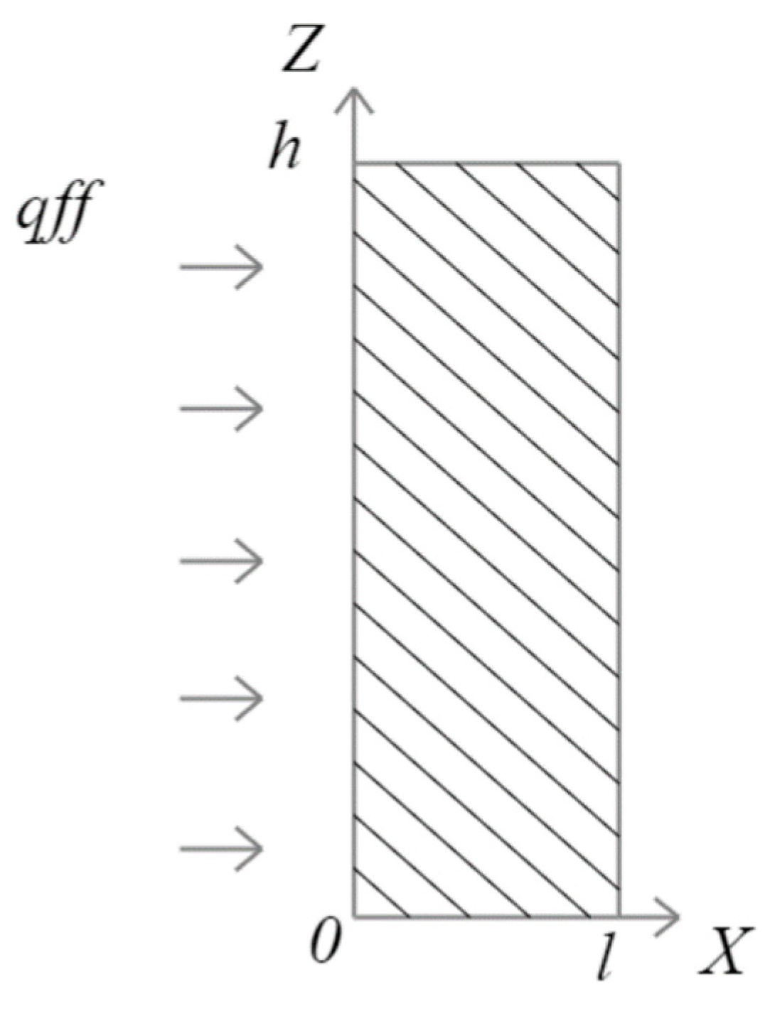
  • In the enclosing structures, heat exchange is carried out by the heat conduction mechanism;
  • Two-dimensional setting;
  • The shape of the fire front is a parabola;
  • Thermophysical properties of building materials do not depend on temperature;
  • A catastrophic scenario of fire weather is assumed when there is no moisture in the surface layer of the wall;
  • Disregard wood pyrolysis;
  • The main mechanism of heat transfer from the line of fire to the building is heat radiation;
  • The temperature of the forest fire front is taken into account using the Stefan-Boltzmann law;
  • The impact of the forest fire front on the wall is determined by qff and Tff.
The wooden structure is under the influence of the heat flow from the forest fire front qff. On the surface of the fence exposed to the heat flow from the forest fire front, the material itself becomes a radiation source.
The physical model diagram is shown in Figure 1.
For the numerical solution of the differential equation of heat conduction, the finite difference method described in [64,65] was used:
ρ c T t = x ( λ T x ) + y ( λ T y ) + z ( λ T z ) + Q w ( x , y , z , T )
where ρ, c, λ, T are the density, heat capacity, heat conduction coefficient and temperature; Qw is the heat source inside the decision area; t is the temporal coordinate; x, y, z are the spatial coordinates.
An implicit difference scheme was used for the solution. The left boundary condition was used to determine the coefficients α and β from the relation
T 1 = α 1 T 2 + β 1 ,
where T1, T2 are the temperature in computational mesh nodes number 1 and 2; α1 is the first running coefficient number 1; β1 is the second running coefficient number 1.
The right boundary condition is used to determine the temperature at the boundary x = L; for the number of nodes N, the temperature at the boundary will have the form TN(K). The boundary conditions have been discredited to the first order of approximation. It is assumed that a forest fire front is approaching the structure from the left side. Convection-radiation heat transfer at the boundary of the enclosing structure is calculated as an approximation on the left and right boundaries.
On the left border:
λ 1 T 1 x | x = 0 = α ( T f f T 1 ) + ε σ ( T f f 4 T 1 4 ) + q f f
where T1 is the temperature in the first node of computational mesh; Tff is the temperature in the fire front; λ1 is heat conduction coefficient of first layer of the enclosing construction of the wall; α is the heat transfer coefficient; ε is the emissivity factor; σ is the Stefan–Boltzmann constant; qff is the heat flux from fire line; x is the spatial coordinate.
Then:
{ α 1 = λ 1 λ 1 + h α β 1 = h α T f f + ε σ h ( T f f 4 T 1 4 ) + h q f f λ 1 + h α
where α1 is the first running coefficient; β1 is the second running coefficient; λ1 is the heat conduction coefficient of the first layer of enclosing construction of the wall; α is the heat transfer coefficient; ε is the emissivity factor; σ is the Stefan–Boltzmann constant; qff is the heat flux from fire line; T1 is the temperature in the first node of computational mesh; Tff is the temperature in the fire front; h is the spatial step in x-direction.
On the right border, the temperature is equal to the indoor temperature, boundary conditions of the first kind:
λ 2 T 2 x | x = x N = α ( T 2 T e ) ,
where T2 is the temperature in the second layer of the enclosing construction of the wall; Te is the temperature of the indoor environment of the object; xN is the thickness of the wall; λ2 is the heat conduction coefficient of the second layer of enclosing construction of the wall; α is the heat transfer coefficient; x is the spatial coordinate.
Since there is a nonlinear component on the left boundary, heating according to the Stefan–Boltzmann law, to refine the temperature on the left boundary, it is necessary to use the method of simple iterations. To take into account the temperature distribution over depth, a two-dimensional mathematical model was used.
The mathematical model is represented by a two-dimensional non-stationary heat conduction equation.
ρ 1 c 1 T 1 t = λ 1 2 T 1 x 2 + λ 1 2 T 1 y 2 + q f f exp ( k ρ 1 x ) ,
ρ 2 c 2 T 2 t = λ 2 2 T 2 x 2 + λ 2 2 T 2 y 2 ,
The left border is exposed to radiant heat flux:
x = 0 ; λ 1 T 1 x = k 1 q f f + ε σ ( T f f 4 T 1 4 ) ,
x = x N ; λ 2 T 2 x = α ( T 2 T e ) ,
y = 0 ; λ i T i y = 0 ,
y = y N ; λ i T i y = 0 ,
Initial conditions:
T i | t = 0 = T i 0 ,
The formula for calculating the heat flux of the front of the surface forest fire [61]:
q f f = ( q f d + x f 50 d q f h ) / 2 ,
The formula for calculating the heat flux of the front of a crown forest fire [61]:
q f f = ( q f d + t exp x f 10 d q f h ) / 2 ,
As a result of processing data on the falling heat fluxes from the forest fire front [61], equations were obtained. These equations are most consistent with the experimental data [66].
Dependence of heat flux on distance [66]:
q f d = 1000 326.37 exp ( 0.2791 x f ) ,   kW / m 2 ,
Dependence of heat flux on flame height [66]:
q f h = 1000 ( 16.638 x f + 29.772 ) ,   kW / m 2 ,
where ρi, ci, λi, Ti are the density, heat capacity, heat conduction coefficient and temperatures in the first and second layers of the enclosing construction of wall; Te is the indoor environment temperature; qff is the resulting heat flux from fire front; qfd is the heat flux component depending on distance from wall to fire front; qfh is the heat flux component depending on fire front height; k is the coefficient for law that similar to Bouguer–Lambert–Beer law; ε is the emissivity factor; σ is the Stefan–Boltzmann constant; α is the heat transfer coefficient; xf is the current distance from wall to fire front until the end of exposure; d is the initial distance from wall to fire front; x, y are the spatial coordinates; t is the temporal coordinate; texp is the exposure time from fire front.

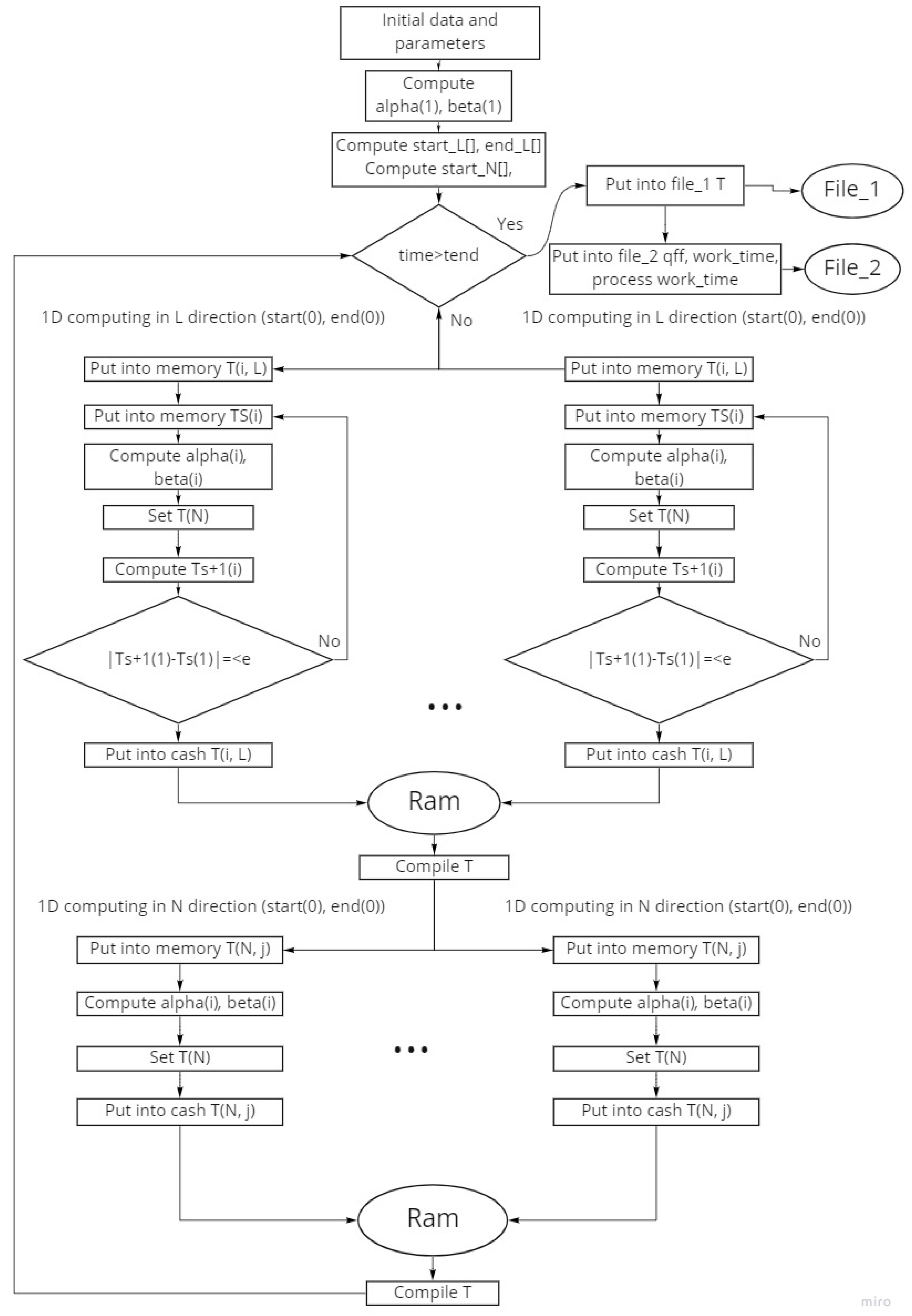
4. Parallel Implementation

To implement parallel computing in Python 3.x, the multiprocessing module was used. This module allows us to conveniently start many processes asynchronously. At the beginning of the program in the synchronous mode, the variables required for the calculation are initialized. The values α1 and β1 are also calculated, arrays of initial values of the temperature field and coordinate axes are created and filled. After that, the nodes are evenly divided into sections along the X and Z axes. After dividing the computational grid, the start and end points of the process are set for each process. The processes are launched within the specified ranges along the Z axis with accuracy L (Figure 2). During the process, locally one-dimensional problems are solved for each L(n) included in the range L(start, end).
In a case when the number of nodes is divided by the number of processes without a remainder, the smallest matrix is calculated in the process that is launched last. In this case, the result of the last process can be put into memory before the rest. For this, the results of the calculations of the processes enters the memory with the indication of the index of the process in which they were calculated.
At the moment, in the process, the temperature field T(i, L) is being calculated where L(start, end) are determined by the number of processes, and i is the indices of an element in an array of length N (Figure 3). The boundary conditions at the boundary T(N, L) are also redefined using the method of simple iterations, and the surface temperature TS(i) is recalculated for each i-th node along N. At the time the process is running, the data processed by the process is placed in RAM and the process index is assigned to them, so after all processes are finished, the full computational grid with the calculated sections for each process is stored in memory. Further, the data obtained as a result of the work of each process is combined in memory. The file memory data is collected into a matrix, which is transposed for ease of use, and unnecessary sections that have not been processed by the process are removed. From these data, a final data set is collected, which corresponds to a matrix with the same surface as the initial temperature field. Next, the matrix is transposed and placed in processes to perform an X-axis run. Now the processes are launched within the specified ranges along the X axis with accuracy N. In the process, locally one-dimensional problems are solved for each N(n) included in the range N(start, end).
In this case, the process calculates the temperature field T(N, j) where N is determined by the number of processes, and j is the indices of the element in the array of length L. As a result of the process, the collected matrix is recalculated along the perpendicular coordinate axis, and the data is written into memory. After that, the data from memory is cleared of sections that did not take part in the process. A common matrix is then assembled. After that, the total matrix is placed in memory, but already in another variable with the index of the time iteration. After the condition t > tend is fulfilled, a dictionary in which the key is the time iteration and the value of the array of temperature values at this iteration, the matrix is placed in a JSON file, and a file is created with logs on the total running time of the algorithm, heat fluxes, the lifetime of each process, and initial conditions. A block diagram is presented in Figure 4.
When the computing system consists of the node (M = 1), the time of cycle performance is
T 0 = p N V c ,
where p is the number of operations that are necessary to calculate one cycle iteration, NV is the number of cycle iterations, c is the node productivity.
Then if NV > M and NV is divided by M without a reminder, the cycle iterations N V M are carried out on each processor. The time of cycle performance is
T M = p N V M c ,
Acceleration SM can be defined using relationship T0 to TM and, as a result, obtain
S M = M ,
This formula is proven for acceleration and is fair in full absence of losses.
The efficiency of parallel computing is calculated using the formulas presented in [67]:
E = T 0 M T M ,
where T0 is the calculation time in sequential mode, TM is the calculation time using M processes. This ratio allows you to calculate the efficiency factor without taking into account losses.
In the case when during the operation of the algorithm, there are performance losses for creating and closing processes, as well as losses for data exchange. In this case, the process running time will be described by the T’M parameter. Efficiency is calculated using the formula [67]:
E = T 0 M T M = T 0 M ( T M 0 + α T M 0 ) = 1 ( 1 + α M )
α M = T M T M 0
Acceleration can be calculated using the formula [67]:
S M = M ( 1 + α M ) ,
The calculations were performed on a multiprocessor cluster in the Sirius University of Science and Technology, which consists of 40 computing nodes (Dell PowerEdge R640 Server) and one management server (Dell PowerEdge R640 Server), interconnected using an Infiniband computer network and an Ethernet network for monitoring and managing jobs. Computing nodes are numbered continuously in the form “cn-X” (where X is a number from 001 to 040).
Each computational node includes:
  • 2 Intel Xeon Gold 6140 processors, 2.3 GHz, 18 cores/36 threads, 10.4 GT/s, 24.75 MB cache, Turbo, HT (140 W), DDR4 2666 MHz.
  • 8 memory modules RDIMM 32 GB, 2666 MT/s.
  • Mellanox Technologies MT27800 ConnectX-5 Single Port Infiniband Adapter, EDR (name ib0 within host or cn-X-ib0 within cluster).
  • Dual Port Ethernet NIC—Intel Corporation Ethernet Controller X710 for 10GbE SFP + (eth0).
  • SATA 200 GB.
The control node of the computing cluster consists of:
  • 2 Intel Xeon Gold 5118 processors, 2.3 GHz, 18 cores/36 threads, 10.4 GT/s, 24.75 MB cache, Turbo, HT (140 W), DDR4 2666 MHz.
  • 8 memory modules RDIMM 32 GB, 2666 MT/s.
  • Mellanox Technologies MT27800 ConnectX-5 Single Port Adapter Infiniband, EDR (name ib0 within the host or nodeXXX-ib0 within the cluster).
  • Dual Port Ethernet NIC—Intel Corporation Ethernet Controller X710 for 10GbE SFP + (em0).
  • Dual Port Ethernet NIC—I350 Gigabit Network Connection (em3).
  • 4 SAS disks 1.8 TB, 10,000 rpm
The parallel program is written in Python 3.x. Anaconda version 4.6.2 was used as an interpreter since parallel settlement is performed within one main process. Then the efficiency is considered for each of the calculation blocks separately.
Figure 5 shows how the efficiency of a parallel program depends on the number of processes involved in the calculation for the first computational block.
Figure 6 shows how the efficiency of a parallel program depends on the number of processes involved in the calculation for the second computational block.
The actual efficiency decreases in comparison with the estimated one. This may be due to the fact that the operating time of the function called by the process is less than the time of the process call, and in this case, with a further increase in the number of processes, the efficiency will not increase, but will only decrease.
With a further increase in the number of processes, the total execution time is expected to decrease; however, after 16 processes, the efficiency begins to decrease, since the acceleration on each individual process can no longer cover the increase in the time for data merging.
The dependence of the acceleration on the program of the first block is shown in Figure 7.
The dependence of the acceleration on the program of the second block is shown in Figure 8.
The real speedup is slightly less than the estimated one, since a fraction of the time is lost when sending data at the beginning and when collecting results at the end of the parallel program execution. It seems that the speedup decreases as the number of processors increases, although the computational load on each process decreases.
Figure 9 shows the total running time of the algorithm in relation to the synchronous implementation. The relative time was chosen to determine the dependence of the execution time on the number of processes in general.
Although the execution time of each individual process decreases as the number of processes increases, the total time for 2 processes in relation to 1 process increases. The increase in total time when working with 2 processes can be explained by the fact that data fusion takes a lot of time, and therefore the time savings on each separate process are not significant.
However, we managed to get a productivity increase of 29% for 8 and 16 processes. A further increase in the number of processes leads to a slowdown in the calculation and is not advisable. Thus, we can conclude that the most effective application of the algorithm is the parallelization of subtasks within the framework of parallel calculation of various input data.
The considered algorithm is well suited for parallel implementation using multiprocessor systems; however, calibration is required by the number of processes and the amount of input data. Efficiency depends on the number of processes and its change can have a positive and negative direction.

5. Results and Discussion

To carry out test calculations and the possibility of further validation of the algorithm, we used the scenarios from [61]. During the modeling process, three types of forest fires were considered. A surface forest fire of low intensity, characterized by a low front height, about 1 m and a low propagation speed of 0.015 m/s over a layer of ground forest fuel. For the second type, a surface forest fire of high intensity, was adopted that fire was characterized by a higher flame height of about 1.5 m and an increased propagation velocity of 0.05 m/s. The main distinguishing feature of a high-intensity surface forest fire from a low-intensity one is that of a high-intensity fire. The increased height of the flame leads to an increase in the speed of movement of the forest fire front. The last type is a crown forest fire, the height of the flame reaches the height of the tree crowns. Due to the greatly increased height of the flame, the propagation speed increases and is 0.33 m/s. A thin wall with a thickness of 0.02 m was considered as the enclosing structure. This thickness was adopted because the heating of wood during a fire does not occur by more than 0.02 m [61,68]. A low-intensity forest fire front starts to move at a distance of 20 m from the enclosing structure. The material of construction is plywood. The front speed is set at 0.015 m/s, the flame height is 1 m. The estimated time is 425 s. The calculation results are shown in Figure 10.
A high-intensity surface forest fire front starts to move at a distance of 20 m from the enclosing structure. The material of construction is plywood. The front speed is set to 0.05 m/s, the flame height is 1.5 m. The estimated time is 350 s. The calculation time is recorded less; in our discussion of the results it is described in detail why this is so. The calculation results are shown in Figure 11.
The front of the crown forest fire begins to move at a distance of 20 m from the enclosing structure. The material of construction is plywood. The front speed is set to 0.33 m/s, the flame height is from 1 m to 10 m. The estimated time is 50 s. The calculation results are shown in Figure 12.
A low-intensity surface forest fire front begins to move at a distance of 20 m from the enclosing structure. The material of construction changes for each calculation. The front speed is set to 0.015 m/s, the flame height is 1 m. The estimated time is 425 s. The calculation results are shown in Figure 13.
A high-intensity surface forest fire front starts to move at a distance of 20 m from the enclosing structure. The material of construction changes for each calculation. The front speed is set at 0.05 m/s, the flame height is 1 m. The estimated time is 350 s. The calculation results are shown in Figure 14.
The effect of paint and varnish coatings was found to be small, the temperature difference on the surface was about 2 °C. The data on the absorption coefficients of radiant energy for various paints are used in civil engineering. Data are given on unpainted wood species, dark gray paint, white and blue paint, and also on a straw-colored surface [62]. The material is considered as a material made of plywood.
As a result of numerous computational experiments, similar to [61] patterns of the impact of forest fires on the enclosing structures of a wooden building were obtained. The first group of computational experiments examined the effects of various forest fires on a wall made from unpainted wood materials. As it was established as a result of modeling, the wall heats up mainly at the stage preceding the ignition, and heating occurs in the surface layers of wood with a thickness of about 2 cm.
Temperature distributions in the plywood enclosure were obtained. The results are shown in Figure 10. Although the propagation speed is not high, the surface temperature exceeds 800 °C for an exposure time of 425 s. The results disagree with the results in [61]. This discrepancy can be caused by the feature of rounding numbers in different programming language; the feature of parallel calculation.
A high intensity surface forest fire has a significant effect on surface temperature. After 350 s of exposure, the temperature at the boundary and the heat flux reaches their limit values, and the boundary condition can no longer be calculated. This phenomenon can be associated with the fact that the wood begins to smolder and give off to the environment a heat flux equal to the heat flux from the forest fire front and no further heating occurs. In a crown fire, the critical temperature is reached within one minute of exposure. Critical temperatures are reached in the range of heights from 1 to 10 m. Temperature fields were calculated in various materials of construction.
Figure 13 shows the temperature distribution over the depth of the material. The scenario of a low-intensity ground forest fire was considered. The exposure time is 425 s. As can be seen in Figure 13, the maximum heating of the material corresponds to pine wood. The least effect of heat flow is observed for facing cardboard and fiberboard with a density of 1000 kg/m3. Temperatures reach critical values, while the falling heat flux is not large.
Figure 14 shows the temperature distribution over the depth of the material. A scenario of a high-intensity surface forest fire was considered. The exposure time is 350 s since further recalculation of the boundary conditions does not occur. The temperatures at the border are above critical. In this case, ignition of the structure is inevitable.
A crown forest fire was not considered, since in the event of such a fire developing near the building, the owner can only be saved through evacuation.
Thus, it can be seen that the ignition of the structures of a wooden building occurs in a fairly short exposure time. The computation time of the sequential prediction algorithm is longer than the ignition time of structures under the scenarios presented in this work. The demand for reducing the simulation time is extremely high, otherwise such models will not be of practical importance. Possible ways to reduce the simulation time include a decrease in the resolution of the computational grid, which will cause a significant drop in the simulation accuracy; at sufficiently low resolutions, the temperature data in the near-surface layer can differ several times, which is unacceptable. The second option considered in this paper is distributed computing. With parallel calculations, it is possible to achieve the speed of calculating temperature fields on computational grids with a high resolution comparable to the speed of calculating temperature fields with a low resolution. With a low accuracy of calculating the temperature fields, parallel calculations will not have advantages, but on the contrary will be inferior in speed to a simple synchronous algorithm, since the operating time of each individual process will be less than the calculation time, and a further increase in the calculation processes will increase the operating time of the algorithm presented in the work by value 2n, where n is the number of additional processes involved in the calculation. High-resolution calculations require large amounts of RAM, since it must simultaneously contain full-size matrices for correct calculation in each process. Also, the requirements for the volumes of hard drives, which must be fast enough, are increasing.
The most correct direction for the development of parallel calculations is probably the development of algorithms that in parallel counted several detached buildings with different scenarios of the effect of the heat flux from the forest fire front on the enclosing structures. These algorithms, in conjunction with GIS systems, are able to quickly simulate the impact of a forest fire on entire settlements near the WUI.
It is necessary to check the results obtained in this article in comparison with the previously published data from [61]. Three series of comparative analyzes were carried out. It should be noted that in [61], a three-dimensional formulation is considered, implemented using a sequential programming model, which imposed restrictions on the number of nodes in the computational grid in space and time. In the present article, a two-dimensional formulation is considered, implemented in the SPMD-model of computations using the parallelization of computational operations. The first series completely repeated the conditions for carrying out mathematical modeling in [61], except that in this article a two-dimensional formulation was used. The second series of comparative analysis was carried out for conditions when the reflection of radiation from the wall surface was not taken into account, whereas in [61] this was taken into account. The third series of comparative analysis was carried out for conditions when the penetration of radiation into the surface layer of the cladding was taken into account in this work, similar to the Bouguer–Lambert–Beer law. Several scenarios were considered:
Scenario 1. Impact of a low intensity surface forest fire on a glued plywood wall from a distance of 20 m.
Scenario 2. Exposure of a high intensity surface forest fire to a glued plywood wall from a distance of 20 m.
Scenario 3. Impact of a crown forest fire at different heights on a glued plywood wall from a distance of 20 m.
The results of the comparative analysis are shown in the Table 4.
Taking into account the penetration of radiation into the depth of the cladding layer noticeably changes the values of the calculated temperature, both on the surface and in the depth of the cladding layer. Fundamental differences were noted for the scenario of the impact of a low-intensity surface forest fire. A comparative analysis of the results shows that the danger of a low-intensity surface forest fire cannot be underestimated. It is necessary, as with other types of forest fires, to take measures to preserve the lives and property of homeowners. Compared to other forest fires, a low-intensity surface forest fire is characterized by the lowest rate of propagation over a layer of ground forest fuels. This gives homeowners time to evacuate the forest fire area and to rescue documents and valuables.

6. Conclusions

As a result of the work, an algorithm for the implementation of parallel calculations of heat transfer processes inside a wooden enclosing structure under the influence of thermal radiation from the forest fire front was developed and tested.
The dependencies show similarities with the work [44]. However, they have different numerical values. These discrepancies can be caused by different rounding methods in different programming languages.
The speed of work turned out to be contradictory. On the one hand, there is an increase in productivity, but with an increase in processes over 16, a slowdown in calculation is observed.
Thus, the developed algorithm is of great practical importance. By distributing the load on different processors, the calculation speed of the model is reduced. This makes it possible to apply more complex complex mathematical models and improve the accuracy of the computational grid. It also opens up room for experiments for the simultaneous calculation of problems with different initial conditions and conditions for the flow of heat transfer processes. Further development will make it possible to apply these algorithms when calculating the fire hazard of an entire settlement under various conditions of the impact of a forest fire front on the structure of buildings.
The main advantage of the developed program code is explained by the possibility of applying this code to large areas of research. This article considers a narrow example of the application of the developed code to a simple two-dimensional problem of the impact of a forest fire on a two-layer enclosing structure of an infrastructure facility of Russian Railways. In the next phase of research, the developed program code will be applied to a two-dimensional research area representing an entire street of a railway station, which is approaching a forest fire front. At the third stage of research, remote sensing data on a specific infrastructure facility of Russian Railways in the Republic of Buryatia (Russian Federation) will be connected. Retrospective data from Landsat and Sentinel 2A satellites will be used.

Author Contributions

Conceptualization, N.V.B.; methodology, N.V.B. and A.P.; software, A.P. and A.M.; validation, A.P. and A.M.; formal analysis, N.V.B. and A.M.; investigation, N.V.B., A.P. and A.M.; resources, A.P.; data curation, N.V.B. and A.M.; writing—original draft preparation, N.V.B., A.P. and A.M.; writing—review and editing, N.V.B.; visualization, N.V.B., A.P. and A.M.; supervision, N.V.B.; project administration, N.V.B.; funding acquisition, N.V.B. All authors have read and agreed to the published version of the manuscript.

Funding

The reported study was funded by RFBR, Sirius University of Science and Technology, JSC Russian Railways and Educational Fund “Talent and success”, project number 20-31-51001. The APC was funded by RFBR, Sirius University of Science and Technology, JSC Russian Railways and Educational Fund “Talent and success”, project number 20-31-51001.

Institutional Review Board Statement

Not applicable.

Informed Consent Statement

Not applicable.

Data Availability Statement

Data can be provided by the request for author.

Conflicts of Interest

The authors declare no conflict of interest.

References

  1. McNamee, M.; Meacham, B.; van Hees, P.; Bisby, L.; Chow, W.K.; Coppalle, A.; Weckman, B. IAFSS agenda 2030 for a fire safe world. Fire Saf. J. 2019, 110, 102889. [Google Scholar] [CrossRef]
  2. Liu, D.; Xu, Z.; Wang, Z.; Zhou, Y.; Fan, C. Estimation of effective coverage rate of fire station services based on real-time travel times. Fire Saf. J. 2021, 120, 103021. [Google Scholar] [CrossRef]
  3. Calkin, D.E.; Gebert, K.M.; Jones, J.G.; Neilson, R.P. Forest service large fire area burned and suppression expenditure trends, 1970–2002. J. For. 2005, 103, 179–183. [Google Scholar] [CrossRef]
  4. Short, K.C. A spatial database of wildfires in the United States, 1992–2011. Earth Syst. Sci. Data 2014, 6, 1–27. [Google Scholar] [CrossRef] [Green Version]
  5. Monedero, S.; Ramírez, J.; Molina-Terrén, D.; Cardil, A. Simulating wildfires backwards in time from the final fire perimeter in point-functionalfire models. Environ. Model. Softw. 2017, 92, 163–168. [Google Scholar] [CrossRef]
  6. Zárate, L.; Arnaldos, J.; Casal, J. Establishing safety distances for wildland fires. Fire Saf. J. 2008, 43, 565–575. [Google Scholar] [CrossRef]
  7. Bao, T.; Liu, S.; Qin, Y.; Liu, Z.L. 3D modeling of coupled soil heat and moisture transport beneath a surface fire. Int. J. Heat Mass Transf. 2019, 149, 119163. [Google Scholar] [CrossRef]
  8. Certini, G. Effects of fire on properties of forest soils: A review. Oecologia 2005, 143, 1–10. [Google Scholar] [CrossRef]
  9. Knicker, H. How does fire affect the nature and stability of soil organic nitrogen and carbon? A review. Biogeochemistry 2007, 85, 91–118. [Google Scholar] [CrossRef]
  10. González-Pérez, J.A.; Gonzalez-Vila, F.J.; Almendros, G.; Knicker, H. The effect of fire on soil organic matter—A review. Environ. Int. 2004, 30, 855–870. [Google Scholar] [CrossRef]
  11. Massman, W.J.; Frank, J.M.; Mooney, S.J. Advancing investigation and physical modeling of first-order fire effects on soils. Fire Ecol. 2010, 6, 36–54. [Google Scholar] [CrossRef]
  12. Peinl, P. A retrospective on ASPires—An advanced system for the prevention and early detection of forest fires. Internet Things 2021, 100456. [Google Scholar] [CrossRef]
  13. Hirsch, K.; Martell, D. A review of initial attack fire crew productivity and effectiveness. Int. J. Wildland Fire 1996, 6, 199–215. [Google Scholar] [CrossRef]
  14. Frangieh, N.; Accary, G.; Rossi, J.-L.; Morvan, D.; Meradji, S.; Marcelli, T.; Chatelon, F.-J. Fuelbreak effectiveness against wind-driven and plume-dominated fires: A 3D numerical study. Fire Saf. J. 2021, 124, 103383. [Google Scholar] [CrossRef]
  15. Klimont, Z.; Kupiainen, K.; Heyes, C.; Purohit, P.; Cofala, J.; Rafaj, P.; Borken-Kleefeld, J.; Schöpp, W. Global anthropogenic emissions of particulate matter including black carbon. Atmos. Chem. Phys. Discuss. 2017, 17, 8681–8723. [Google Scholar] [CrossRef] [Green Version]
  16. Kadir, E.A.; Rosa, S.L.; Syukur, A.; Othman, M.; Daud, H. Forest fire spreading and carbon concentration identification in tropical region Indonesia. Alex. Eng. J. 2021. [Google Scholar] [CrossRef]
  17. Thomas, G.; Rosalie, V.; Olivier, C.; Maria, D.G.A.; Antonio, L.P. Modelling forest fire and firebreak scenarios in a mediterranean mountainous catchment: Impacts on sediment loads. J. Environ. Manag. 2021, 289, 112497. [Google Scholar] [CrossRef]
  18. Mizukami, T.; Utiskul, Y.; Quintiere, J.G. A compartment burning rate algorithm for a zone model. Fire Saf. J. 2016, 79, 57–68. [Google Scholar] [CrossRef]
  19. Zhu, Q.; Liu, Y.; Jia, R.; Hua, S.; Shao, T.; Wang, B. A numerical simulation study on the impact of smoke aerosols from Russianforestfires on the air pollution over Asia. Atmos. Environ. 2018, 182, 263–274. [Google Scholar] [CrossRef]
  20. Miller, C.; Urban, D.L. Connectivity of forest fuels and surface fire regimes. Landsc. Ecol. 2000, 15, 145–154. [Google Scholar] [CrossRef]
  21. Loehle, C. Applying landscape principles to fire hazard reduction. For. Ecol. Manag. 2004, 198, 261–267. [Google Scholar] [CrossRef] [Green Version]
  22. Ager, A.A.; Day, M.A.; Finney, M.A.; Vance-Borland, K.; Vaillant, N.M. Analyzing the transmission of wildfire exposure on a fire-prone landscape in Oregon, USA. For. Ecol. Manag. 2014, 334, 377–390. [Google Scholar] [CrossRef]
  23. Schertzer, E.; Staver, A.C.; Levin, S. Implications of the spatial dynamics of fire spread for the bistability of savanna and forest. J. Math. Biol. 2015, 70, 329–341. [Google Scholar] [CrossRef] [PubMed]
  24. Oliveira, T.M.; Barros, A.M.G.; Ager, A.A.; Fernandes, P.M. Assessing the effect of a fuel break network to reduce burnt area and wildfire risk transmission. Int. J. Wildland Fire 2016, 25, 619–632. [Google Scholar] [CrossRef]
  25. Viedma, O.; Angeler, D.G.; Moreno, J.M. Landscape structural features control fire size in a Mediterranean forested area of central Spain. Int. J. Wildland Fire 2009, 18, 575–583. [Google Scholar] [CrossRef]
  26. Luo, M.; He, Y.; Beck, V. Application of field model and two-zone model to flashover fires in a full-scale multi-room single level building. Fire Saf. J. 1997, 29, 1–25. [Google Scholar] [CrossRef]
  27. Rein, G.; Bar-Ilan, A.; Fernandez-Pello, A.C.; Alvares, N. A comparison of three models for the simulation of accidental fires. J. Fire Prot. Eng. 2006, 16, 183–209. [Google Scholar] [CrossRef]
  28. McGrattan, K.; Baum, H.; Rehm, R. Large eddy simulations of smoke movement. Fire Saf. J. 1998, 30, 161–178. [Google Scholar] [CrossRef]
  29. Yeoh, G.; Yuen, R.; Chueng, S.; Kwok, W. On modelling combustion, radiation and soot processes in compartment fires. Build. Environ. 2003, 38, 771–785. [Google Scholar] [CrossRef]
  30. Keramida, E.P.; Boudouvis, A.G.; Lois, E.; Markatos, N.; Karayannis, A.N. Evaluation of two radiation models in CFD fire modeling. Numer. Heat Transf. Appl. 2001, 39, 711–722. [Google Scholar] [CrossRef]
  31. D’Amico, D.F.; Quiring, S.M.; Maderia, C.M.; McRoberts, D.B. Improving the hurricane outage prediction model by includingtree species. Clim. Risk Manag. 2019, 25, 100193. [Google Scholar] [CrossRef]
  32. Liu, D.; Xu, Z.; Fan, C. Predictive analysis of fire frequency based on daily temperatures. Nat. Hazards 2019, 97, 1175–1189. [Google Scholar] [CrossRef]
  33. Li, P.; Zhao, W. Image fire detection algorithms based on convolutional neural networks. Case Stud. Therm. Eng. 2020, 19, 100625. [Google Scholar] [CrossRef]
  34. Liu, D.; Xu, Z.; Zhou, Y.; Fan, C. Heat map visualisation offire incidents based on transformed sigmoid risk model. Fire Saf. J. 2019, 109, 102863. [Google Scholar] [CrossRef]
  35. Xu, Z.; Liu, D.; Yan, L. Temperature-based fire frequency analysis using machine learning: A case of Changsha, China. Clim. Risk Manag. 2021, 31, 100276. [Google Scholar] [CrossRef]
  36. Kwon, B.; Ejaz, F.; Hwang, L.K. Machine learning for heat transfer correlations. Int. Commun. Heat Mass Transf. 2020, 116, 104694. [Google Scholar] [CrossRef]
  37. Plourde, F.; Doan-Kim, S.; Dumas, J.; Malet, J. A new model of wildland fire simulation. Fire Saf. J. 1997, 29, 283–299. [Google Scholar] [CrossRef]
  38. Novozhilov, V.; Moghtaderi, B.; Fletcher, D.; Kent, J. Computational fluid dynamics modelling of wood combustion. Fire Saf. J. 1996, 27, 69–84. [Google Scholar] [CrossRef]
  39. Morvan, D.; Dupuy, J.L. Modeling of fire spread through a forest fuel bed using a multiphase formulation. Combust. Flame 2001, 127, 1981–1984. [Google Scholar] [CrossRef]
  40. Mell, W.; Maranghides, A.; McDermott, R.; Manzello, S.L. Numerical simulation and experiments of burning Douglasfir trees. Combust. Flame 2009, 156, 2023–2041. [Google Scholar] [CrossRef]
  41. Bufacchi, P.; Krieger, G.C.; Mell, W.; Alvarado, E.; Santos, J.C.; Carvalho, J.A. Numerical simulation of surface forest fire in Brazilian Amazon. Fire Saf. J. 2016, 79, 44–56. [Google Scholar] [CrossRef] [Green Version]
  42. Renane, R.; Chetehouna, K.; Séro-Guillaume, O.; Nour, A.; Rudz, S. Numerical simulations of laminar burning velocities of a major volatile organic compound involved in accelerating forest fires. Appl. Therm. Eng. 2013, 51, 670–676. [Google Scholar] [CrossRef]
  43. Singh, K.R.; Neethu, K.; Madhurekaa, K.; Harita, A.; Mohan, P. Parallel SVM model for forest fire prediction. Soft Comput. Lett. 2021, 3, 100014. [Google Scholar] [CrossRef]
  44. Hegedűs, F.; Krähling, P.; Lauterborn, W.; Mettin, R.; Parlitz, U. High-performance GPU computations in nonlinear dynamics: An efficient tool for new discoveries. Meccanica 2020, 55, 2493–2504. [Google Scholar] [CrossRef] [Green Version]
  45. Pandya, S.B.; Patel, R.H.; Pandya, A.S. Evaluation of power consumption of entry-level and mid-range multi-core mobile processor. In Proceedings of the 4th International Conference on Electronics, Communications and Control Engineering, Seoul, Korea, 9–11 April 2021; pp. 32–39. [Google Scholar]
  46. Ma, Z.; Hong, K.; Gu, L. Volume: Enable large-scale in-memory computation on commodity clusters. In Proceedings of the 2013 IEEE 5th International Conference on Cloud Computing Technology and Science, Bristol, UK, 2–5 December 2013; pp. 56–63. [Google Scholar]
  47. Brun, C.; Artés, T.; Cencerrado, A.; Margalef, T.; Cortés, A. A high performance computing framework for continental-scale forest fire spread prediction. Procedia Comput. Sci. 2017, 108, 1712–1721. [Google Scholar] [CrossRef]
  48. Innocenti, E.; Silvani, X.; Muzy, A.; Hill, D.R. A software framework for fine grain parallelization of cellular models with OpenMP: Application to fire spread. Environ. Model. Softw. 2009, 24, 819–831. [Google Scholar] [CrossRef]
  49. Karafyllidis, I. Design of a dedicated parallel processor for the prediction of forest fire spreading using cellular automata and genetic algorithms. Eng. Appl. Artif. Intell. 2004, 17, 19–36. [Google Scholar] [CrossRef]
  50. Bianchini, G.; Caymes-Scutari, P.; Méndez-Garabetti, M. Evolutionary-statistical system: A parallel method for improving forest fire spread prediction. J. Comput. Sci. 2015, 6, 58–66. [Google Scholar] [CrossRef]
  51. Asllanaj, F.; Contassot-Vivier, S.; Botella, O.; França, F.H. Numerical solutions of radiative heat transfer in combustion systems using a parallel modified discrete ordinates method and several recent formulations of WSGG model. J. Quant. Spectrosc. Radiat. Transf. 2021, 274, 107863. [Google Scholar] [CrossRef]
  52. Kuleshov, A.; Chetverushkin, B.; Myshetskaya, E. Parallel computing in forest fires two-dimension modeling. Comput. Fluids 2013, 80, 202–206. [Google Scholar] [CrossRef]
  53. Emerson, D.R.; Ecer, A.; Periaux, J.; Satoruka, N.; Fox, P. Parallel simulation of forest fire spread due to firebrand transport. In Parallel Computational Fluid Dynamics ’97: Recent Developments and Advances Using Parallel Computers; Emerson, D., Fox, P., Satofuka, N., Ecer, A., Periaux, J., Eds.; North Holland: Haarlem, The Netherlands, 1998; pp. 115–121. [Google Scholar]
  54. Caymes-Scutari, P.; Tardivo, M.L.; Bianchini, G.; Méndez-Garabetti, M. Dynamic Tuning of a Forest Fire Prediction Parallel Method. Communications in Computer and Information Science; 1184 CCIS; CACIC: Río Cuarto, Argentina, 2019; pp. 19–34. [Google Scholar] [CrossRef]
  55. Artés, T.; Cencerrado, A.; Cortés, A.; Margalef, T. Relieving the effects of uncertainty in forest fire spread prediction by hybrid MPI-OpenMP parallel strategies. Procedia Comput. Sci. 2013, 18, 2278–2287. [Google Scholar] [CrossRef] [Green Version]
  56. Cencerrado, A.; Artés, T.; Cortes, A.; Margalef, T. Relieving uncertainty in forest fire spread prediction by exploiting multicore architectures. Procedia Comput. Sci. 2015, 51, 1752–1761. [Google Scholar] [CrossRef] [Green Version]
  57. Denham, M.; Laneri, K. Using efficient parallelization in graphic processing units to parameterize stochastic fire propagation models. J. Comput. Sci. 2018, 25, 76–88. [Google Scholar] [CrossRef] [Green Version]
  58. The Open MPI Organization. Open MPI: Open Source High Performance Computing. Available online: https://www.open-mpi.org/ (accessed on 20 October 2021).
  59. The OpenMP API Specification for Parallel Programming. Available online: https://www.openmp.org/ (accessed on 29 September 2021).
  60. CUDA Toolkit. Available online: https://developer.nvidia.com/cuda-toolkit (accessed on 29 September 2021).
  61. Baranovskiy, N.; Malinin, A. Mathematical simulation of forest fire impact on industrial facilities and wood-based buildings. Sustainability 2020, 12, 5475. [Google Scholar] [CrossRef]
  62. Gosstroy. Thermal Performance of the Buildings; Gosstroy: Moscow, Russia, 2003. (In Russian) [Google Scholar]
  63. Zabolotnyi, A.E.; Zabolotnaya, M.M.; Timoshin, V.N. Determining the regions of safe use of solidfuel generators of fire-extinguishing aerosols. Issues Spec. Eng. 1995, 7, 15–22. (In Russian) [Google Scholar]
  64. Samarskii, A.A.; Vabishchevich, P.N. Computational Heat Transfer; Volume 1: Mathematical Modelling; Wiley: Chichester, UK, 1995; p. 418. [Google Scholar]
  65. Samarskii, A.A.; Vabishchevich, P.N. Computational Heat Transfer; Volume 2: The Finite Difference Method; Wiley: Chichester, UK, 1995; p. 432. [Google Scholar]
  66. Valendik, E.N.; Kosov, I.V. Effect of thermal radiation of forest fire on the environment. Contemp. Probl. Ecol. 2008, 1, 399–403. [Google Scholar] [CrossRef]
  67. Baranovskiy, N.V. Forest fire danger assessment using SPDM-model of computation for massive parallel system. Int. Rev. Modeling Simulation. 2017, 10, 193–201. [Google Scholar]
  68. Baranovskiy, N.V.; Malinin, A. Mathematical simulation of forest fire front influence on wood-based building using one-dimensional model of heat transfer. E3S Web Conf. 2020, 200, 03007. [Google Scholar] [CrossRef]
Figure 1. Scheme of the physical model.
Algorithms 14 00333 g001
Figure 2. Scheme of parallelization of the calculation along the L axis.
Algorithms 14 00333 g002
Figure 3. Scheme of parallelization of the calculation along the N axis.
Algorithms 14 00333 g003
Figure 4. Block diagram of the algorithm.
Algorithms 14 00333 g004
Figure 5. The efficiency of parallel implementation for the first block of calculations.
Algorithms 14 00333 g005
Figure 6. The efficiency of parallel implementation for the second block of calculations.
Algorithms 14 00333 g006
Figure 7. Dependence of acceleration on the program of the first block.
Algorithms 14 00333 g007
Figure 8. Dependence of acceleration on the program of the second block.
Algorithms 14 00333 g008
Figure 9. Total running time of the algorithm depending on the number of processes.
Algorithms 14 00333 g009
Figure 10. Impact of a surface forest fire (low intensity) on plywood from a distance of 20 m—temperature distribution along the wall thickness.
Algorithms 14 00333 g010
Figure 11. Impact of a surface forest fire (high intensity) on plywood from a distance of 20 m—temperature distribution along the wall thickness.
Algorithms 14 00333 g011
Figure 12. Impact of a crown forest fire on plywood from a distance of 20 m for different facade heights (from 1 to 10 m).
Algorithms 14 00333 g012
Figure 13. Impact of surface forest fires (low intensity) on various materials from a distance of 20 m in 425 s of exposure—temperature distribution over the wall thickness.
Algorithms 14 00333 g013
Figure 14. Impact of surface forest fires (high intensity) on various materials from a distance of 20 m for 350 s of exposure—temperature distribution along the wall thickness.
Algorithms 14 00333 g014
Table 1. Thermophysical characteristics of materials [62].
Material λ , W m K c , J k g K ρ , k g m 3
Pine wood0.121670500
Birch wood0.282200440
Glued plywood0.122300600
Cardboard0.1823001000
Fiberboard (1000)0.1523001000
Fiberboard (800)0.132300800
Table 2. Experimental data on wood ignition by radiant heat flux [63].
Ignition Delay, sHeat Flux to the Surface, kW/m2Surface Temperature, K
63.512.5658
45.021700
11.142726
2.684773
0.4210867
Table 3. Absorption coefficients for different types of paint [62].
PaintAbsorption Coefficient
Pure wood0.6
Gray0.7
White0.3
Blue0.6
Straw-colored0.45
Table 4. Comparative analysis of the results of numerical modeling (deviation of the numerical results from the sequential version [61], average difference).
ScenarioSeries 1Series 2Series 3
1 (surface temperature)10%15%210%
1 (in-depth temperature)13%18%212%
2 (surface temperature)12%14%12%
2 (in-depth temperature)17%19%22%
3 (surface temperature)13%15%27%
3 (in-depth temperature)15%17%29%
Publisher’s Note: MDPI stays neutral with regard to jurisdictional claims in published maps and institutional affiliations.

