
Squeezing Backbone Feature Distributions to the Max for Efficient Few-Shot Learning


1
Orange S.A., F-84100 Paris, France
2
IMT Atlantique, Lab-STICC, UMR CNRS 6285, F-29238 Brest, France
*
Author to whom correspondence should be addressed.
Algorithms 2022, 15(5), 147; https://0-doi-org.brum.beds.ac.uk/10.3390/a15050147
Submission received: 8 April 2022
/
Revised: 21 April 2022
/
Accepted: 21 April 2022
/
Published: 26 April 2022
(This article belongs to the Special Issue Algorithms for Machine Learning and Pattern Recognition Tasks)
Abstract
:In many real-life problems, it is difficult to acquire or label large amounts of data, resulting in so-called few-shot learning problems. However, few-shot classification is a challenging problem due to the uncertainty caused by using few labeled samples. In the past few years, many methods have been proposed with the common aim of transferring knowledge acquired on a previously solved task, which is often achieved by using a pretrained feature extractor. As such, if the initial task contains many labeled samples, it is possible to circumvent the limitations of few-shot learning. A shortcoming of existing methods is that they often require priors about the data distribution, such as the balance between considered classes. In this paper, we propose a novel transfer-based method with a double aim: providing state-of-the-art performance, as reported on standardized datasets in the field of few-shot learning, while not requiring such restrictive priors. Our methodology is able to cope with both inductive cases, where prediction is performed on test samples independently from each other, and transductive cases, where a joint (batch) prediction is performed.
1. Introduction
Thanks to their outstanding performance, deep learning methods have been widely considered for vision tasks such as image classification and object detection. In order to reach top performance, these systems are typically trained using very large labeled datasets that are representative enough of the inputs to be processed afterward.
However, in many applications, it is costly to acquire or annotate data, resulting in the impossibility of creating such large labeled datasets. Under this condition, it is challenging to optimize deep learning architectures considering the fact they typically are made of way more parameters than the dataset can efficiently tune. This is the reason why in the past few years, few-shot learning (i.e., the problem of learning with few labeled examples) has become a trending research subject in the field. In more detail, there are two settings that authors often consider: (a) “inductive few-shot”, where only a few labeled samples are available during training, and prediction is performed on each test input independently, and (b) “transductive few-shot”, where prediction is performed on a batch of (non-labeled) test inputs, allowing to take into account their joint distribution.
Few-shot learning is critical to many applications. To name a few, it has been considered for vision [1,2,3], audio [4,5,6], language [7,8,9], and medical imaging [10,11,12]. More generally, few-shot learning can be used to provide proofs-of-concept while limiting the costs of data labeling or to help in pseudo-annotation of datasets. This importance of the problem of few-shot learning explains the abundant literature across the recent years.
Many works in the domain are built based on a “learning to learn” guidance, where the pipeline is to train an optimizer [13,14,15] with different tasks of limited data so that the model is able to learn generic experience for novel tasks. Namely, the model learns a set of initialization parameters that are in an advantageous position for the model to adapt to a new (small) dataset. Recently, the trend evolved towards using well-thought-out feature extractors, called backbones [1,2,16,17,18,19], that are trained one time on a large generic dataset in order to produce easily classified feature vectors.
A main problem of the existing methods is that they typically require priors about the data balance between considered classes to perform at their best [1,20]. These methods could be patched to work efficiently under other regimes but would still require the knowledge of data distribution between classes. In this work, we introduce a new methodology with a double aim: 1—providing state-of-the-art performance, as reported using standardized benchmarks in the field of few-shot learning, and 2—not requiring any priors about data distribution among classes.
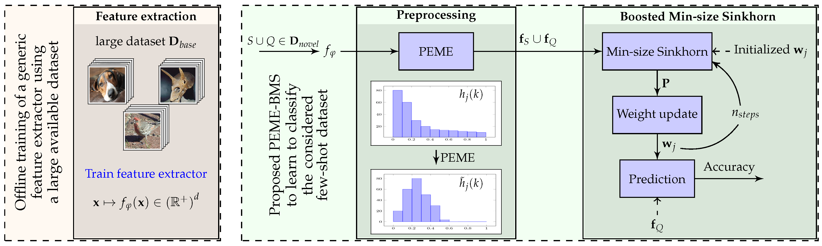
To achieve this goal, we introduce a novel methodology, summarized in Figure 1, that combines feature preprocessing, self-distillation and an optimal transport-based framework. The utility of these ingredients is demonstrated using ablation tests.
The outline of the paper is as follows. In Section 2, we introduce related work and discuss the novelty of the proposed approach. In Section 3, we introduce the proposed methodology. Section 4 contains several experiments and benchmark results, along with corresponding discussions. Finally, Section 5 presents the conclusion.
2. Related Work
A large volume of works in few-shot classification is based on meta learning [15] methods, where the training data are transformed into few-shot learning episodes to better fit in the context of a few examples. In this branch, optimization-based methods [13,14,15,21,22,23] train a well-initialized optimizer so that it quickly adapts to unseen classes with a few epochs of training. Other works [24,25] apply data augmentation techniques to artificially increase the size of the training data in order for the model to generalize better to unseen data.
In the past few years, there has been a growing interest in transfer-based methods. The main idea consists of training feature extractors able to efficiently segregate novel classes it has never seen. For example, in [2,18], the authors train the backbone with a distance-based classifier [26] that takes into account the inter-class distance. In [2], the authors utilize self-supervised learning techniques [27] to co-train an extra rotation classifier for the output features, improving the accuracy in few-shot settings. More recent works adopt a two-stage training procedure [28,29,30] where the authors first batch-train a model, then use episodic training to better adjust class prototypes. There are also methods that train a model with a combination of different ingredients [31,32], e.g., distillation [33,34] under a teacher-student framework to better find the nuances between samples. Aside from approaches focused on training a more robust model, other approaches are built on top of a pre-trained feature extractor (backbone). For instance, in [35], the authors implement a nearest class mean classifier to associate an input with a class whose centroid is the closest in terms of the distance. In [20], an iterative approach is used to adjust the class prototypes. In [19], the authors build a graph neural network to gather the feature information from similar samples. Generally, transfer-based techniques often reach the best performance on standardized benchmarks.
Although many works involve feature extraction, few have explored the features in terms of their distribution [2,36,37]. Often, assumptions are made that the features in a class align to a certain distribution, even though these assumptions are seldom experimentally discussed. In our work, we analyze the impact of the feature distributions and how they can be transformed for better processing and accuracy. We also introduce a new algorithm to improve the quality of the association between input features and corresponding classes in typical few-shot settings.
Let us highlight the main contributions of this work. (1) We propose a novel preprocessing method to be applied to raw extracted features in order to make them more aligned with Gaussian assumptions. (2) We introduce a Wasserstein-based method to better align the distribution of features with that of the considered classes and combine it with self-distillation. (3) We show that the proposed method can bring a large increase in accuracy with a variety of feature extractors and datasets, leading to state-of-the-art results in the considered benchmarks. This work is an extended version of [1], with the main difference that here we consider the broader case where we do not know the proportion of samples belonging to each considered class in the case of a transductive few-shot, leading to a new algorithm called the Boosted Min-size Sinkhorn. We also propose more efficient preprocessing steps, leading to overall better performance in both inductive and transductive settings. Finally, we introduce the use of logistic regression with self-distillation in our methodology instead of a simple nearest class mean classifier.
3. Materials and Methods
In this section, we introduce the problem statement. We also discuss the various steps of the proposed method, including training the feature extractors, preprocessing the feature representations, and classifying them. Note that we made the code of our method available at https://github.com/yhu01/BMS (accessed on 1 February 2022).
3.1. Problem Statement
We consider a typical few-shot learning problem. Namely, we are given a base dataset and a novel dataset such that . contains a large number of labeled examples from K different classes and can be used to train a generic feature extractor. , also referred to as a task or episode in other works, contains a small number of labeled examples (support set ), along with some unlabeled ones (query set ), all from n new classes that are distinct from the K classes in . Our goal is to predict the classes of unlabeled examples in the query set. The following parameters are of particular importance to define such a few-shot problem: the number of classes in the novel dataset n (called n-way), the number of labeled samples per class s (called s-shot) and the number of unlabeled samples per class q. Therefore, the novel dataset contains a total of samples, where are labeled, and are unlabeled. In the case of an inductive few-shot, the prediction is performed independently on each one of the query samples. In the case of a transductive few-shot [20,38], the prediction is performed considering all unlabeled samples together. Contrary to our previous work [1], we do not consider knowing the proportion of samples in each class in the case of a transductive few-shot.
3.2. Feature Extraction
The first step is to train a neural network backbone model using only the base dataset. In this work, we consider multiple backbones with various training procedures. Once the considered backbone is trained, we obtain robust embeddings that should generalize well to novel classes. We denote by the backbone function, obtained by extracting the output of the penultimate layer from the considered architecture, with being the trained architecture parameters. Thus, considering an input vector , is a feature vector with d dimensions that can be thought of as a simpler-to-manipulate representation of . Note that, importantly, in all backbone architectures used in the experiments of this work, the penultimate layers are obtained by applying a ReLU function so that all feature components coming out of are nonnegative.
3.3. Feature Preprocessing
As mentioned in Section 2, many works hypothesize, explicitly or not, that the features from the same class are aligned with a specific distribution (often Gaussian-like). However, this aspect is rarely experimentally verified. In fact, it is very likely that features obtained using the backbone architecture are not Gaussian. Indeed, usually, the features are obtained after applying a ReLU function [39] and exhibit a positive and yet skewed distribution mostly concentrated around 0 (more details can be found in the next section).
Multiple works in the domain [20,35] discuss the different statistical methods (e.g., batch normalization) to better fit the features into a model. Although these methods may have provable assets for some distributions, they could worsen the process if applied to an unexpected input distribution. This is why we propose to preprocess the obtained raw feature vectors so that they better align with typical distribution assumptions in the field. Denote as the obtained features on , and let denote its value in the hth position. The preprocessing methods applied in our proposed algorithms are as follows:
(E) Euclidean normalization. Also known as L2-normalization, which is widely used in many related works [19,35,37], this step scales the features to the same area so that large variance feature vectors do not predominate the others. Euclidean normalization can be given by:
(P) Power transform. The power transform method [1,40] simply consists of taking the power of each feature vector coordinate. The formula is given by:
where = 1 × 10 is used to make sure that is strictly positive in every position, and is a hyper-parameter. The rationale of the preprocessing above is that power transform, often used in combination with euclidean normalization, has the functionality of reducing the skew of the distribution and mapping it to a close-to-Gaussian distribution, adjusted by . After experiments, we found that gives the most consistent results for our considered experiments, which corresponds to a square-root function that has a wide range of usage on features [41]. We will analyze this ability and the effect of power transform in more detail in Section 4. Note that power transform can only be applied if considered feature vectors contain nonnegative entries, which will always be the case in the remainder of this work.
(M) Mean subtraction. With mean subtraction, each sample is translated using , the projection center. This is often used in combination with euclidean normalization in order to reduce the task bias and better align the feature distributions [20]. The formula is given by:
The projection center is often computed as the mean values of feature vectors related to the problem [20,35]. In this paper, we compute it either as the mean feature vector of the base dataset (denoted as ) or the mean vector of the novel dataset (denoted as ), depending on the few-shot settings. Of course, in both of these cases, the rationale is to consider a proxy to what would be the exact mean value of feature vectors on the considered task.
In our proposed method, we deploy these preprocessing steps in the following order: Power transform (P) on the raw features, followed by a Euclidean normalization (E). Then, we perform mean subtraction (M) followed by another Euclidean normalization at the end. The resulting abbreviation is PEME, in which M can be either or , as mentioned above. In our experiments, we found that using in the case of inductive few-shot learning and in the case of transductive few-shot learning consistently led to the most competitive results. More details on why we used this methodology are available in the experiment section.
When facing an inductive problem, a simple classifier such as a Nearest-Class-Mean classifier (NCM) can be used directly after this preprocessing step. The resulting methodology is denoted PEE-NCM. However, in the case of transductive settings, we also introduce an iterative procedure, denoted BMS for Boosted Min-size Sinkhorn, meant to leverage the joint distribution of unlabeled samples. The resulting methodology is denoted PEE-BMS. The details of the BMS procedure are presented thereafter.
3.4. Boosted Min-Size Sinkhorn
In the case of transductive few-shot, we introduce a method that consists of iteratively refining estimates for the probability each unlabeled sample belongs to any of the considered classes. This method is largely based on the one we introduced in [1], except it does not require priors about sample distributions in each of the considered classes. Denoting as the sample index in and as the class index, the goal is to maximize the following log post-posterior function:
Here, denotes the class label for sample , denotes the marginal probability, and represents the model parameters to estimate. Assuming a Gaussian distribution on the input features for each class, here we define where stand for the weight parameters for class j. We observe that Equation (4) can be related to the cost function utilized in optimal transport [42], which is often considered to solve classification problems, with constraints on the sample distribution over classes. To that end, a well-known Sinkhorn [43] mapping method is proposed. The algorithm aims at computing a class allocation matrix among novel class data for a minimum Wasserstein distance. Namely, an allocation matrix is defined where denotes the assigned portion for sample i to class j, and it is computed as follows:
where is a set of positive matrices for which the rows sum to and the columns sum to , denotes the distribution of the amount that each sample uses for class allocation, and denotes the distribution of the amount of samples allocated to each class. Therefore, contains all the possible ways of allocation. In the same equation, can be viewed as a cost matrix that is of the same size as , each element in indicates the cost of its corresponding position in . We will define the particular formula of the cost function for each position in details later on in the section. As for the second term on the right of (5), it stands for the entropy of : , regularized by a hyper-parameter . Increasing would force the entropy to become smaller, so that the mapping is less diluted. This term also makes the objective function strictly convex [43,44] and thus a practical and effective computation. From lemma 2 in [43], the result of the Sinkhorn allocation has the typical form . It is worth noting that here we assume a soft class allocation, meaning that each sample can be “sliced” into different classes. We will present our proposed method in detail in the following paragraphs.
Given all that is presented above, in this paper, we propose an Expectation–Maximization (EM) [45] based method, which alternates between updating the allocation matrix and estimating the parameter of the designed model, in order to minimize Equation (5) and maximize Equation (4). For a starter, we define a weight matrix with n columns (i.e., one per class) and d rows (i.e., one per dimension of feature vectors), and for column j in , we denote it as the weight parameters for class j in correspondence with Equation (4). It is initialized as follows:
where
We can see that contains the average of feature vectors in the support set for each class, followed by a L2-normalization on each column so that .
Then, we iterate multiple steps that we describe thereafter.
- a
- Computing costs
As previously stated, the proposed algorithm is an EM-like one that iterately updates model parameters for optimal estimates. Therefore, this step, along with Min-size Sinkhorn presented in the next step, is considered as the E-step of our proposed method. The goal is to find membership probabilities for the input samples; namely, we compute that minimizes Equation (5).
Here, we assume Gaussian distributions, and features in each class have the same variance and are independent from one another (covariance matrix ). We observe that, ignoring the marginal probability, Equation (4) can be boiled down to negative L2 distances between extracted samples and , which is initialized in Equation (6) in our proposed method. Therefore, based on the fact that and are both normalized to be unit length vectors ( being preprocessed using PEME introduced in the previous section), here we define the cost between sample i and class j to be the following equation:
which corresponds to the cosine distance.
- b
- Min-size Sinkhorn
In [1], we proposed a Wasserstein distance-based method in which the Sinkhorn algorithm is applied at each iteration so that the class prototypes are updated iteratively in order to find their best estimates. Although the method showed promising results, it is established on the condition that the distribution of the query set is known, e.g., a uniform distribution among classes on the query set. This is not ideal, given the fact that any priors about should be supposedly kept unknown when applying a method. The methodology introduced in this paper can be seen as a generalization of that introduced in [1] that does not require priors about .
In the classical settings, the Sinkhorn algorithm aims at finding the optimal matrix , given the cost matrix and regulation parameter presented in Equation (4). Typically, it initiates from a softmax operation over the rows in , then it iterates between normalizing columns and rows of , until the resulting matrix becomes close to doubly stochastic according to and . However, in our case, we do not know the distribution of samples over classes. To address this, we firstly introduce the parameter k, initialized so that , meant to track an estimate of the cardinal of the class containing the least number of samples in the considered task. Then, we propose the following modification to be applied to the matrix once initialized: we normalize each row as in the classical case but only normalize the columns of for which the sum is less than the previously computed min-size k [20]. This ensures at least k elements are allocated for each class, but not exactly k samples as in the balanced case.
The principle of this modified Sinkhorn solution is presented in Algorithm 1.
| Algorithm 1 Min-size Sinkhorn |
|
- c
- Updating weights
This step is considered as the M-step of the proposed algorithm, in which we use a variant of the logistic regression algorithm in order to find the model parameter in the form of weight parameters for each class. Note that , if normalized, is equivalent to the prototype for class j in this case. Given the fact that in Equation (4), we also take into account the marginal probability, it can be further broken down as:
We observe that Equation (4) corresponds to applying a softmax function on the negative logits computed through an L2-distance function between samples and class prototypes (normalized). This fits the formulation of a linear hypothesis between and for logit calculations, hence the rationale for utilizing logistic regression in our proposed method. Note that contrary to classical logistical regression, we implement here a form of self-distillation. Indeed, we use soft labels contained in instead of one-hot class indicator targets, and these targets are refined iteratively.
The procedure of this step is as follows: now that we have a polished allocation matrix , we firstly initialize the weights as follows:
where
We can see that elements in are used as coefficients for feature vectors to linearly adjust the class prototypes [1]. Similar to Equation (6), here is the normalized newly-computed class prototype that is a vector of length 1.
Next, we further adjust weights by applying a logistic regression, and the optimization is performed by minimizing the following loss:
where contains the logits, and each element is computed as:
Note that is a scaling parameter, it can also be seen as a temperature parameter that adjusts the confidence metric to be associated with each sample. It is learnt jointly with .
The deployed logistic regression comes with hyperparameters on its own. In our experiments, we use an SGD optimizer with a gradient step of and as the momentum parameter, and we train over e epochs. Here, we point out that is considered an influential hyperparameter in our proposed algorithm, indicates a simple update of as the normalized adjusted class prototypes (Equation (10)) computed from in Equation (11), without further adjustment of logistic regression. In addition, note that when , we project columns of to the unit hypersphere at the end of each epoch.
- d
- Estimating the class minimum size
We can now refine our estimate for the min-size k for the next iteration. To this end, we firstly compute the predicted label of each sample as follows:
which can be seen as the current (temporary) class prediction.
Then, we compute:
where , representing the cardinal of a set.
Summary of the proposed method: all steps of the proposed method are summarized in Algorithm 2. In our experiments, we also report the results obtained when using a prior about as in [1]. In this case, k does not have to be estimated throughout the iterations and can be replaced with the actual exact targets for the Sinkhorn. We denote this prior-dependent version PEE-BMS* (with an added *).
| Algorithm 2 Boosted Min-size Sinkhorn (BMS) |
3.5. Implementation Details
In order to stress the genericity of our proposed method with regards to the chosen backbone architecture and training strategy, we perform experiments using WRN [46], ResNet18 and ResNet12 [47], along with some other pretrained backbones (e.g., DenseNet [35,48]). For each dataset, we train the feature extractor with base classes and test the performance using novel classes. Therefore, for each test run, n classes are drawn uniformly at random among novel classes. Among these n classes, s labeled examples and q unlabeled examples per class are uniformly drawn at random to form . The WRN and ResNet are trained following [2]. In the inductive setting, we use our proposed preprocessing steps PEE followed by a basic Nearest Class Mean (NCM) classifier. In the transductive setting, the preprocessing steps are denoted as PEE in that we use the mean vector of a novel dataset for mean subtraction, followed by BMS or BMS* depending on whether we have prior knowledge onf the distribution of query set among classes. Note that we perform a QR decomposition on preprocessed features in order to speed up the computation for the classifier that follows. All our experiments are performed using , or 5. In our experiments, we perform 10,000 random runs to obtain the mean accuracy score and indicate confidence scores () when relevant. For our proposed PEE-BMS, we train epoch in the case of 1-shot and epochs in the case of 5-shot. As for PEE-BMS*, we set for 1-shot and for 5-shot. As for the regularization parameter in Equation (5), it is fixed to for all settings. The impact of these hyperparameters is detailed in the next sections.
4. Results and Discussions
4.1. Comparison with State-of-the-Art Methods
Performance on standardized benchmarks: in the first experiment, we conduct our proposed method on different benchmarks and compare the performance with other state-of-the-art solutions. The results are presented in Table 1 and Table 2, and we observe that our method reaches the state-of-the-art performance in both inductive and transductive settings on all the few-shot classification benchmarks. Particularly, the proposed PEE-BMS* brings important gains in both 1-shot and 5-shot settings, and the prior-independent PEE-BMS also obtains competitive results on 5-shot. Note that for tieredImageNet we implement our method based on a pre-trained DenseNet121 backbone following the procedure described in [35]. From these experiments, we conclude that the proposed method can bring an increase in accuracy with a variety of backbones and datasets, leading to a state-of-the-art performance. In terms of execution time, we measured an average of 0.004 s per run. These results confirm the ability of the proposed methodology to reach state-of-the-art performance using the standardized benchmarks of the field of few-shot learning.
Performance on cross-domain settings: in this experiment, we test our method in a cross-domain setting, where the backbone is trained with the base classes in miniImageNet but tested with the novel classes in the CUB dataset. As shown in Table 3, the proposed method gives the best accuracy both in the case of 1-shot and 5-shot, for both inductive and transductive settings. The ability of the proposed methodology to leverage feature vectors trained on a different dataset points out that its efficacy is not restricted to constrained settings where data distribution between the base and novel have to be identical.
4.2. Ablation Studies
Ablation study on the proposed method: in this section, we have a closer look at the impact of our proposed methodology steps. The idea is to better understand the contribution of each step to the final performance. Namely, we conduct an ablation study on the prediction accuracy with or without (1) PEME, which is the proposed preprocessing steps on extracted raw features, and (2) proposed Boosted Min-sized Sinkhorn algorithm that integrates self-distillation for refined prototypes. Note that in the case of BMS*, the algorithm is equivalent to MAP presented in [1] without the newly proposed self-distillation method. In Table 4, we can see that both PEME and self-distillation play an important role in improving the prediction performance. As such, this experiment supports the interest of both steps to reach the best possible accuracy.
Generalization to backbone architectures. To further stress the interest of the ingredients inn the proposed method reaching top performance, in Table 5 we investigate the impact of our proposed method on different backbone architectures and benchmarks in the transductive setting. For comparison purposes, we also replace our proposed BMS algorithm with a standard K-Means algorithm where class prototypes are initialized with the available labeled samples for each class. We can observe that: (1) the proposed method consistently achieves the best results for any fixed backbone architecture, (2) the feature extractor trained on WRN outperforms the others with our proposed method on different benchmarks, (3) there are significant drops in accuracy with k-means, which stresses the interest of BMS, and (4) the prior on (BMS vs. BMS*) is of major interest for 1-shot, boosting the performance by an approximation of on all tested feature extractors. Overall, these experiments demonstrate the interest of the proposed methodology with respect to existing alternatives.
Preprocessing impact: in Table 6, we compare our proposed feature preprocessing PEME with other preprocessing techniques such as batch normalization, which standardizes extracted feature values into for a considered task, along with other ones being used in [35]. The experiment is conducted on miniImageNet (backbone: WRN). For all that is put into comparison, we run either an NCM classifier or BMS after preprocessing, depending on the settings. The obtained results clearly show the interest of PEME compared with existing alternatives, and we also observe that the power transform helps increase the accuracy on both inductive and transductive settings.
Effect of power transform: we firstly conduct a Gaussian hypothesis test on each of the 640 coordinates of raw extracted features (backbone: WRN) for each of the 20 novel classes (dataset: miniImageNet). Following D’Agostino and Pearson’s methodology [61,62] and , only one of the tests return positive, suggesting a very low pass rate for raw features. However, after applying the power transform, we record a pass rate that surpasses , suggesting a considerably increased number of positive results for Gaussian tests. This experiment shows the effect of power transform being able to adjust feature distributions into more Gaussian-like ones.
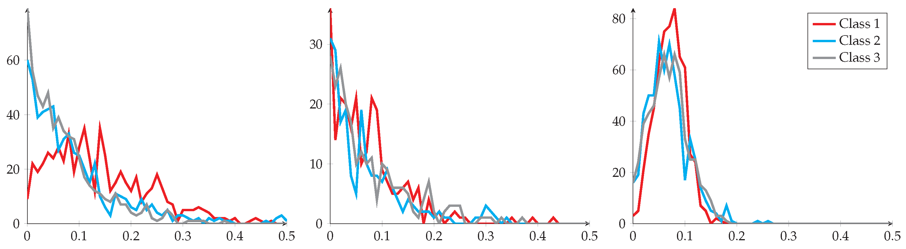
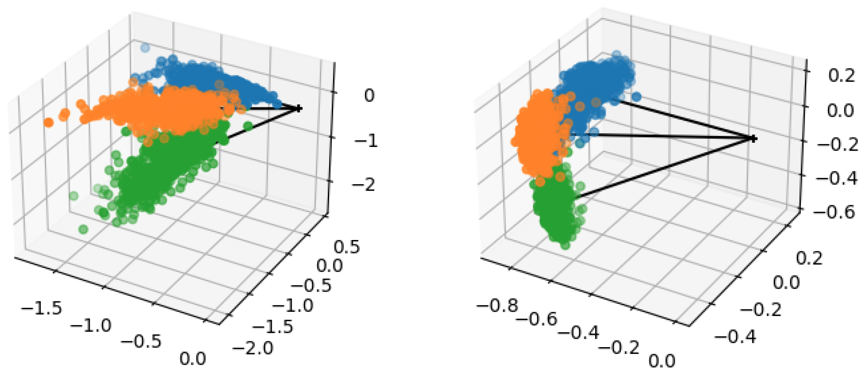
To better show the effect of this proposed technique on feature distributions, we depict in Figure 2 the distributions of an arbitrarily selected feature for three randomly selected novel classes of miniImageNet when using WRN, before and after applying the power transform. In addition, we also added to the figure the feature distributions after applying batch normalization for comparison purposes. We observe quite clearly that (1) raw features exhibit a positive distribution mostly concentrated around 0, a similar behavior is also observed for batch norm, and (2) power transform is able to reshape the feature distributions to close-to-Gaussian distributions. We observe similar behaviors with other datasets as well. Moreover, in order to visualize the impact of this technique with respect to the position of feature points, in Figure 3, we plot the feature vectors of three randomly selected classes from . Note that all feature vectors in this experiment are reduced to 3-dimensional ones corresponding to their largest eigenvalues. From Figure 3, we can observe that the power transform, often followed by an L2-normalization, can help shape the class distributions to become more gathered and Gaussian-like [57].
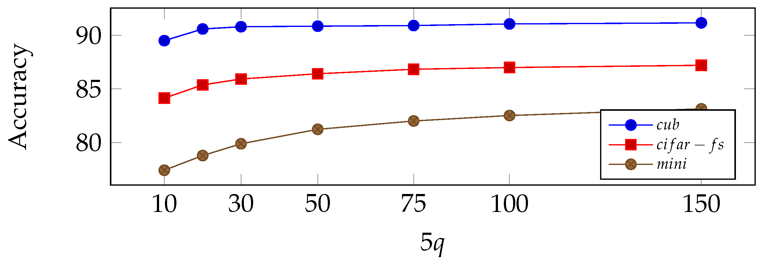
Influence of the number of unlabeled samples: in order to better understand the gain in accuracy due to having access to more unlabeled samples, we depict in Figure 4 the evolution of accuracy as a function of q, when the number of classes is fixed. Interestingly, the accuracy quickly reaches a close-to-asymptotical plateau, emphasizing the ability of the method to quickly exploit available information in the task.
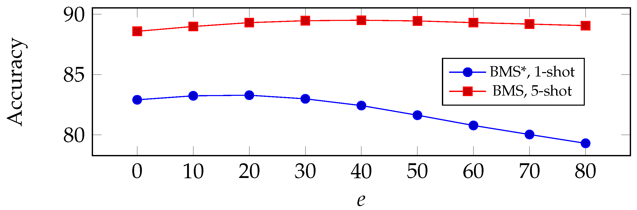
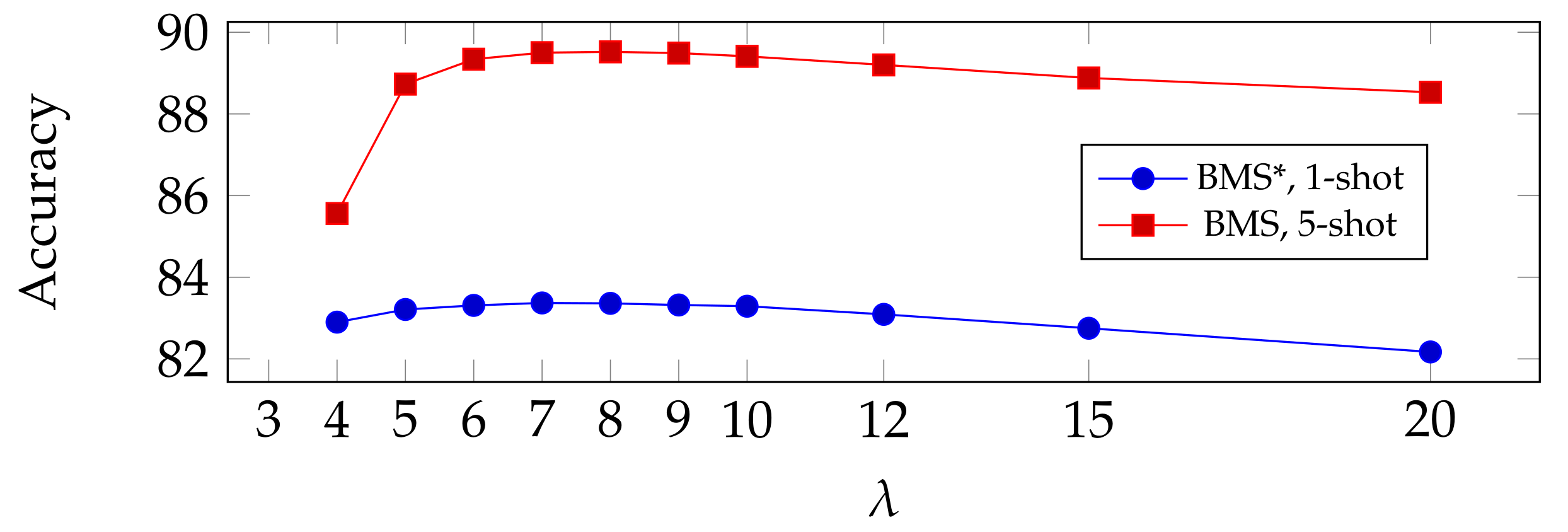
Influence of hyperparameters: in order to test how much impact the hyperparameters could have on our proposed method in terms of prediction accuracy, here we select two important hyperparameters that are used in BMS and observe their impact. Namely, the number of training epochs e in logistic regression and the regulation parameter used for computing the prediction matrix . In Figure 5, we show the accuracy of our proposed method as a function of e (top) and (bottom). Results are reported for BMS* in 1-shot settings, and for BMS in 5-shot settings. From the figure, we can see a slight uptick of accuracy as e or increase, followed by a downhill when they become larger, implying an overfitting of the classifier. We chose our optimal parameters from these experiments. We note that, interestingly, the performance of the method appears quite robust to a non-optimal choice of these parameters.
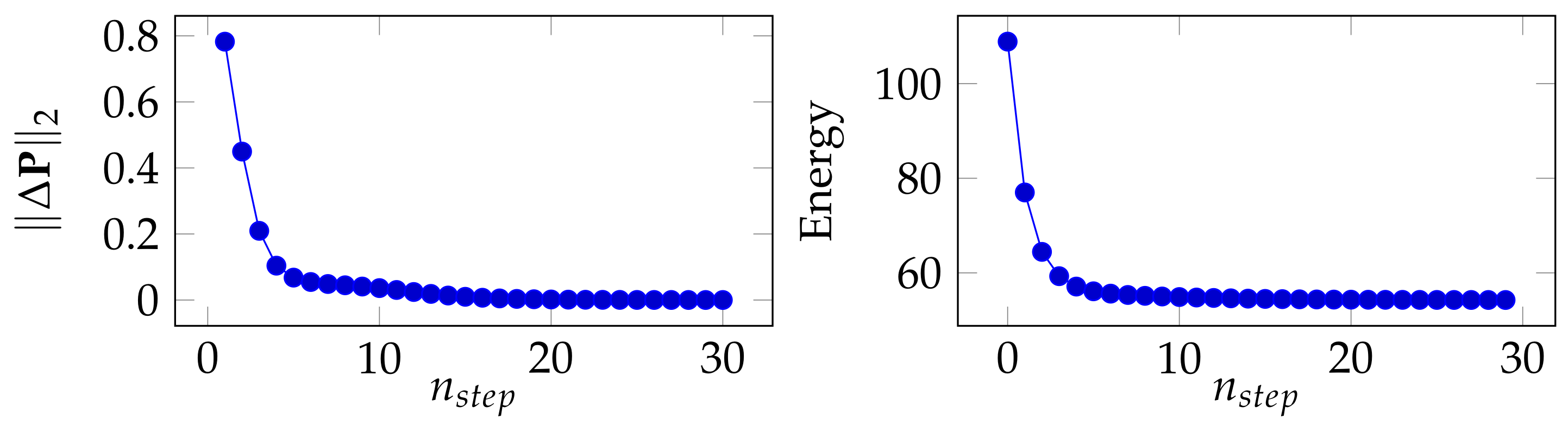
Convergence analysis: in this section, we discuss the convergence of the proposed method in Algorithm 2, namely the convergence of as a function of the number of iteration step noted . We conduct this experiment in a 5-way, 1-shot setting on miniImageNet (backbone: WRN). In Figure 6 (left), we depict as a function of , with being defined as , namely the Euclidean difference between the current and the one computed in the previous step. Furthermore, we remind the reader that the goal of the proposed algorithm is to minimize the energy computed in Equation (5). Therefore, in Figure 6 (right), we depict the energy (value of Equation (5)) as a function of . We can see that both and energy tend to stabilize with more iteration steps.
Proposed method on backbones pre-trained with external data: in this experiment, we compare our proposed method BMS* with the work in [63] that pre-trains the backbone with the help of external illumination data for augmentation, followed by PT + MAP in [1] for class center estimation. Here, we use the same backbones as [63] and replace PT + MAP with our proposed BMS* under the same conditions. Results are presented in Table 7. Note that we also show the re-implemented results of [63], and our method reaches superior performance on all tested benchmarks using external data in [63].
Proposed method on Few-Shot Open-Set Recognition: Few-Shot Open-Set Recognition (FSOR) as a new trending topic deals with the fact that there are open data mixed in query set that do not belong to any of the supposed classes used for label predictions. Therefore, this often requires a robust classifier that is able to correctly classify the non-open data as well as rejecting the open ones. In Table 8, we apply our proposed PEME for feature preprocessing, followed by an NCM classifier and compare the results with other state-of-the-art alternatives. We observe that our proposed method is able to surpass the others in terms of accuracy and AUROC.
4.3. Proposed Method on Merged Features
In this section, we investigate the effect of our proposed method on merged features. Namely, we perform a direct concatenation of raw feature vectors extracted from multiple backbones at the beginning, followed by BMS. In Table 9, we chose the feature vectors from three backbones (WRN, ResNet18 and ResNet12) and evaluated the performance with different combinations. We observe that (1) a direct concatenation, depending on the backbones, can bring about gain in both 1-shot and 5-shot settings compared with the results in Table 5 with feature vectors extracted from one single feature extractor. (2) BMS* reached new state-of-the-art results on few-shot learning benchmarks with feature vectors concatenated from WRN, ResNet18 and ResNet12, given that no external data are used.
To further study the impact of the number of backbones on prediction accuracy, in Figure 7 we depict the performance of our proposed method as a function of the number of backbones. Note that, here, we operate on feature vectors of 6 WRN backbones (dataset: miniImageNet) concatenated one after another, which makes a total of 6 slots corresponding to a feature size. Each of them is trained the same way as in [2], and we randomly select the multiples of 640 coordinates within the slots to denote the number of concatenated backbones used. The performance result is the average of 100 random selections, and we test with both BMS and BMS* for 1-shot, and BMS* for 5-shot. From Figure 7, we observe that, as the number of backbones increases, there is a relatively steady growth in terms of accuracy in multiple settings of our proposed method, indicating the interest of BMS in merged features.
5. Conclusions
In this paper, we introduced a new pipeline to solve the few-shot classification problem. It comes with the two following assets: first, it is able to reach state-of-the-art accuracy on standardized benchmarks of the field, and second, it does not require any explicit priors about data distribution between classes, as opposed to many previous works in the domain. Using extensive experiments, we demonstrated that the proposed methodology can be used in a variety of settings, including cross-domain, multiple backbones, open-set recognition …. Using ablation tests, we showed the importance of the introduced steps in the methodology. The proposed methodology comes with only a few extra hyperparameters, on which our experiments suggest that a fine tuning is not necessarily required. Thus we believe that the proposed method is applicable to many practical engineering problems. In future work, we would like to better understand the fundamental reasons why the proposed preprocessing is able to boost performance. We would also like to find automatic ways to tune the hyperparameters.
Author Contributions
Conceptualization, Y.H., S.P. and V.G.; methodology, Y.H. and S.P.; software, S.P. and V.G.; validation, Y.H., S.P. and V.G.; formal analysis, Y.H., S.P. and V.G.; investigation, Y.H.; resources, S.P. and V.G.; data curation, Y.H.; writing—original draft preparation, Y.H.; writing—review and editing, Y.H., S.P. and V.G.; visualization, Y.H.; supervision, S.P. and V.G.; project administration, S.P. and V.G.; funding acquisition, S.P. All authors have read and agreed to the published version of the manuscript.
Funding
This research was funded by Orange, France.
Institutional Review Board Statement
Not applicable.
Informed Consent Statement
Not applicable.
Data Availability Statement
The data supporting reported results can be found at https://github.com/yhu01/BMS (accessed on 1 February 2022).
Conflicts of Interest
The authors declare no conflict of interest.
References
- Hu, Y.; Gripon, V.; Pateux, S. Leveraging the feature distribution in transfer-based few-shot learning. In Artificial Neural Networks and Machine Learning—ICANN 2021, Proceedings of the 30th International Conference on Artificial Neural Networks, Bratislava, Slovakia, 14–17 September 2021; Springer: Berlin/Heidelberg, Germany, 2021; pp. 487–499. [Google Scholar]
- Mangla, P.; Kumari, N.; Sinha, A.; Singh, M.; Krishnamurthy, B.; Balasubramanian, V.N. Charting the right manifold: Manifold mixup for few-shot learning. In Proceedings of the IEEE Winter Conference on Applications of Computer Vision, Snowmass Village, CO, USA, 1–5 March 2020; pp. 2218–2227. [Google Scholar]
- Wang, X.; Huang, T.E.; Gonzalez, J.; Darrell, T.; Yu, F. Frustratingly Simple Few-Shot Object Detection. In Proceedings of the 37th International Conference on Machine Learning, ICML 2020, Virtual Event, 13–18 July 2020; Volume 119, pp. 9919–9928. [Google Scholar]
- Wang, Y.; Bryan, N.J.; Cartwright, M.; Bello, J.P.; Salamon, J. Few-Shot Continual Learning for Audio Classification. In Proceedings of the IEEE International Conference on Acoustics, Speech and Signal Processing, ICASSP 2021, Toronto, ON, Canada, 6–11 June 2021; pp. 321–325. [Google Scholar]
- Wolters, P.; Careaga, C.; Hutchinson, B.; Phillips, L. A Study of Few-Shot Audio Classification. arXiv 2020, arXiv:2012.01573. [Google Scholar]
- Zhang, S.; Qin, Y.; Sun, K.; Lin, Y. Few-Shot Audio Classification with Attentional Graph Neural Networks. In Interspeech 2019, Proceedings of the 20th Annual Conference of the International Speech Communication Association, Graz, Austria, 15–19 September 2019; Kubin, G., Kacic, Z., Eds.; ISCA: Yuma, AZ, USA, 2019; pp. 3649–3653. [Google Scholar]
- Bansal, T.; Jha, R.; McCallum, A. Learning to Few-Shot Learn Across Diverse Natural Language Classification Tasks. In Proceedings of the 28th International Conference on Computational Linguistics, COLING 2020, Barcelona, Spain, 8–13 December 2020; Scott, D., Bel, N., Zong, C., Eds.; International Committee on Computational Linguistics: Barcelona, Spain, 2020; pp. 5108–5123. [Google Scholar]
- Bansal, T.; Jha, R.; Munkhdalai, T.; McCallum, A. Self-Supervised Meta-Learning for Few-Shot Natural Language Classification Tasks. In Proceedings of the 2020 Conference on Empirical Methods in Natural Language Processing, EMNLP 2020, Online, 16–20 November 2020; Webber, B., Cohn, T., He, Y., Liu, Y., Eds.; Association for Computational Linguistics: Seattle, WA, USA, 2020; pp. 522–534. [Google Scholar]
- Bao, Y.; Wu, M.; Chang, S.; Barzilay, R. Few-shot Text Classification with Distributional Signatures. In Proceedings of the 8th International Conference on Learning Representations, ICLR 2020, Addis Ababa, Ethiopia, 26–30 April 2020. [Google Scholar]
- Sun, L.; Li, C.; Ding, X.; Huang, Y.; Chen, Z.; Wang, G.; Yu, Y.; Paisley, J.W. Few-shot medical image segmentation using a global correlation network with discriminative embedding. Comput. Biol. Med. 2022, 140, 105067. [Google Scholar] [CrossRef] [PubMed]
- Tang, H.; Liu, X.; Sun, S.; Yan, X.; Xie, X. Recurrent mask refinement for few-shot medical image segmentation. In Proceedings of the IEEE/CVF International Conference on Computer Vision, Montreal, QC, Canada, 11–17 October 2021; pp. 3918–3928. [Google Scholar]
- Ouyang, C.; Biffi, C.; Chen, C.; Kart, T.; Qiu, H.; Rueckert, D. Self-supervision with superpixels: Training few-shot medical image segmentation without annotation. In Computer Vision—ECCV 2020, Proceedings of the European Conference on Computer Vision, Glasgow, UK, 23–28 August 2020; Springer: Berlin/Heidelberg, Germany, 2020; pp. 762–780. [Google Scholar]
- Finn, C.; Abbeel, P.; Levine, S. Model-agnostic meta-learning for fast adaptation of deep networks. In Proceedings of the 34th International Conference on Machine Learning, Sydney, Australia, 6–11 August 2017; Volume 70, pp. 1126–1135. [Google Scholar]
- Ravi, S.; Larochelle, H. Optimization as a Model for Few-Shot Learning. In Proceedings of the 5th International Conference on Learning Representations, ICLR 2017, Toulon, France, 24–26 April 2017. [Google Scholar]
- Thrun, S.; Pratt, L. Learning to Learn; Springer Science & Business Media: Berlin/Heidelberg, Germany, 2012. [Google Scholar]
- Torrey, L.; Shavlik, J. Transfer learning. In Handbook of Research on Machine Learning Applications and Trends: Algorithms, Methods, and Techniques; IGI Global: Hershey, PA, USA, 2010; pp. 242–264. [Google Scholar]
- Das, D.; Lee, C.S.G. A Two-Stage Approach to Few-Shot Learning for Image Recognition. IEEE Trans. Image Process. 2020, 29, 3336–3350. [Google Scholar] [CrossRef] [PubMed] [Green Version]
- Chen, W.; Liu, Y.; Kira, Z.; Wang, Y.F.; Huang, J. A Closer Look at Few-shot Classification. In Proceedings of the 7th International Conference on Learning Representations, ICLR 2019, New Orleans, LA, USA, 6–9 May 2019. [Google Scholar]
- Hu, Y.; Gripon, V.; Pateux, S. Graph-based interpolation of feature vectors for accurate few-shot classification. In Proceedings of the 2020 25th International Conference on Pattern Recognition (ICPR), Milan, Italy, 10–15 January 2021; pp. 8164–8171. [Google Scholar]
- Lichtenstein, M.; Sattigeri, P.; Feris, R.; Giryes, R.; Karlinsky, L. Tafssl: Task-adaptive feature sub-space learning for few-shot classification. In Computer Vision—ECCV 2020, Proceedings of the 16th European Conference, Glasgow, UK, 23–28 August 2020; Springer: Berlin/Heidelberg, Germany, 2020; pp. 522–539. [Google Scholar]
- Li, Z.; Zhou, F.; Chen, F.; Li, H. Meta-SGD: Learning to Learn Quickly for Few Shot Learning. arXiv 2017, arXiv:1707.09835. [Google Scholar]
- Antoniou, A.; Edwards, H.; Storkey, A.J. How to train your MAML. In Proceedings of the 7th International Conference on Learning Representations, ICLR 2019, New Orleans, LA, USA, 6–9 May 2019. [Google Scholar]
- Bertinetto, L.; Henriques, J.F.; Torr, P.H.S.; Vedaldi, A. Meta-learning with differentiable closed-form solvers. In Proceedings of the 7th International Conference on Learning Representations, ICLR 2019, New Orleans, LA, USA, 6–9 May 2019. [Google Scholar]
- Zhang, H.; Zhang, J.; Koniusz, P. Few-shot Learning via Saliency-guided Hallucination of Samples. In Proceedings of the IEEE Conference on Computer Vision and Pattern Recognition, Long Beach, CA, USA, 16–20 June 2019; pp. 2770–2779. [Google Scholar]
- Chen, Z.; Fu, Y.; Wang, Y.X.; Ma, L.; Liu, W.; Hebert, M. Image deformation meta-networks for one-shot learning. In Proceedings of the IEEE Conference on Computer Vision and Pattern Recognition, Long Beach, CA, USA, 16–20 June 2019; pp. 8680–8689. [Google Scholar]
- Mensink, T.; Verbeek, J.; Perronnin, F.; Csurka, G. Metric learning for large scale image classification: Generalizing to new classes at near-zero cost. In Computer Vision—ECCV 2012, Proceedings of the European Conference on Computer Vision, Florence, Italy, 7–13 October 2012; Springer: Berlin/Heidelberg, Germany, 2012; pp. 488–501. [Google Scholar]
- Chapelle, O.; Scholkopf, B.; Zien, A. Semi-supervised learning (chapelle, o. et al., eds.; 2006) [book reviews]. IEEE Trans. Neural Netw. 2009, 20, 542. [Google Scholar] [CrossRef]
- Ye, H.J.; Hu, H.; Zhan, D.C.; Sha, F. Few-shot learning via embedding adaptation with set-to-set functions. In Proceedings of the IEEE/CVF Conference on Computer Vision and Pattern Recognition, Seattle, WA, USA, 14–19 June 2020; pp. 8808–8817. [Google Scholar]
- Zhang, C.; Cai, Y.; Lin, G.; Shen, C. DeepEMD: Few-Shot Image Classification with Differentiable Earth Mover’s Distance and Structured Classifiers. In Proceedings of the IEEE/CVF Conference on Computer Vision and Pattern Recognition, Seattle, WA, USA, 14–19 June 2020; pp. 12203–12213. [Google Scholar]
- Kang, D.; Kwon, H.; Min, J.; Cho, M. Relational Embedding for Few-Shot Classification. arXiv 2021, arXiv:2108.09666. [Google Scholar]
- Rizve, M.N.; Khan, S.H.; Khan, F.S.; Shah, M. Exploring Complementary Strengths of Invariant and Equivariant Representations for Few-Shot Learning. In Proceedings of the IEEE Conference on Computer Vision and Pattern Recognition, CVPR 2021, Virtual, 19–25 June 2021; pp. 10836–10846. [Google Scholar]
- Rajasegaran, J.; Khan, S.H.; Hayat, M.; Khan, F.S.; Shah, M. Self-supervised Knowledge Distillation for Few-shot Learning. arXiv 2020, arXiv:2006.09785. [Google Scholar]
- Zhang, Z.; Sabuncu, M.R. Self-Distillation as Instance-Specific Label Smoothing. In Advances in Neural Information Processing Systems 33, Proceedings of the Annual Conference on Neural Information Processing Systems 2020, NeurIPS 2020, Virtual, 6–12 December 2020; Larochelle, H., Ranzato, M., Hadsell, R., Balcan, M., Lin, H., Eds.; MIT Press: Cambridge, MA, USA, 2020. [Google Scholar]
- Tian, Y.; Wang, Y.; Krishnan, D.; Tenenbaum, J.B.; Isola, P. Rethinking Few-Shot Image Classification: A Good Embedding is All You Need? In Computer Vision—ECCV 2020, Proceedings of the 16th European Conference, Glasgow, UK, 23–28 August 2020; Vedaldi, A., Bischof, H., Brox, T., Frahm, J., Eds.; Springer: Berlin/Heidelberg, Germany, 2020; Volume 12359, pp. 266–282. [Google Scholar] [CrossRef]
- Wang, Y.; Chao, W.; Weinberger, K.Q.; van der Maaten, L. SimpleShot: Revisiting Nearest-Neighbor Classification for Few-Shot Learning. arXiv 2019, arXiv:1911.04623. [Google Scholar]
- Gripon, V.; Hacene, G.B.; Löwe, M.; Vermet, F. Improving Accuracy of Nonparametric Transfer Learning via Vector Segmentation. In Proceedings of the 2018 IEEE International Conference on Acoustics, Speech and Signal Processing (ICASSP), Calgary, AB, Canada, 15–20 April 2018; pp. 2966–2970. [Google Scholar]
- Yang, S.; Liu, L.; Xu, M. Free Lunch for Few-shot Learning: Distribution Calibration. In Proceedings of the 9th International Conference on Learning Representations, ICLR 2021, Virtual, 3–7 May 2021. [Google Scholar]
- Liu, Y.; Lee, J.; Park, M.; Kim, S.; Yang, E.; Hwang, S.J.; Yang, Y. Learning to Propagate Labels: Transductive Propagation Network for Few-Shot Learning. In Proceedings of the 7th International Conference on Learning Representations, ICLR 2019, New Orleans, LA, USA, 6–9 May 2019. [Google Scholar]
- Agarap, A.F. Deep Learning using Rectified Linear Units (ReLU). arXiv 2018, arXiv:1803.08375. [Google Scholar]
- Tukey, J.W. Exploratory Data Analysis; Springer: Reading, MA, USA, 1977; Volume 2. [Google Scholar]
- Cinbis, R.G.; Verbeek, J.; Schmid, C. Approximate fisher kernels of non-iid image models for image categorization. IEEE Trans. Pattern Anal. Mach. Intell. 2015, 38, 1084–1098. [Google Scholar] [CrossRef] [PubMed] [Green Version]
- Villani, C. Optimal Transport: Old and New; Springer Science & Business Media: Berlin/Heidelberg, Germany, 2008; Volume 338. [Google Scholar]
- Cuturi, M. Sinkhorn distances: Lightspeed computation of optimal transport. In Advances in Neural Information Processing Systems; MIT Press: Cambridge, MA, USA, 2013; pp. 2292–2300. [Google Scholar]
- Solomon, J.; De Goes, F.; Peyré, G.; Cuturi, M.; Butscher, A.; Nguyen, A.; Du, T.; Guibas, L. Convolutional wasserstein distances: Efficient optimal transportation on geometric domains. ACM Trans. Graph. (TOG) 2015, 34, 1–11. [Google Scholar] [CrossRef]
- Dempster, A.P.; Laird, N.M.; Rubin, D.B. Maximum likelihood from incomplete data via the EM algorithm. J. R. Stat. Soc. Ser. B 1977, 39, 1–22. [Google Scholar]
- Zagoruyko, S.; Komodakis, N. Wide Residual Networks. In Proceedings of the British Machine Vision Conference 2016, BMVC 2016, York, UK, 19–22 September 2016; Wilson, R.C., Hancock, E.R., Smith, W.A.P., Eds.; BMVA Press: York, UK, 2016. [Google Scholar]
- He, K.; Zhang, X.; Ren, S.; Sun, J. Deep residual learning for image recognition. In Proceedings of the IEEE Conference on Computer Vision and Pattern Recognition, Las Vegas, NV, USA, 26 June–1 July 2016; pp. 770–778. [Google Scholar]
- Huang, G.; Liu, Z.; Van Der Maaten, L.; Weinberger, K.Q. Densely connected convolutional networks. In Proceedings of the IEEE Conference on Computer Vision and Pattern Recognition, Honolulu, HI, USA, 21–26 July 2017; pp. 4700–4708. [Google Scholar]
- Vinyals, O.; Blundell, C.; Lillicrap, T.; Wierstra, D. Matching networks for one shot learning. In Advances in Neural Information Processing Systems; MIT Press: Cambridge, MA, USA, 2016; pp. 3630–3638. [Google Scholar]
- Liu, J.; Song, L.; Qin, Y. Prototype rectification for few-shot learning. In Computer Vision—ECCV 2020, Proceedings of the 16th European Conference, Glasgow, UK, 23–28 August 2020; Springer: Berlin/Heidelberg, Germany, 2020; pp. 741–756. [Google Scholar]
- Ziko, I.; Dolz, J.; Granger, E.; Ayed, I.B. Laplacian regularized few-shot learning. In Proceedings of the International Conference on Machine Learning, Vienna, Austria, 12–18 July 2020; pp. 11660–11670. [Google Scholar]
- Boudiaf, M.; Ziko, I.M.; Rony, J.; Dolz, J.; Piantanida, P.; Ayed, I.B. Transductive Information Maximization For Few-Shot Learning. arXiv 2020, arXiv:2008.11297. [Google Scholar]
- Kye, S.M.; Lee, H.; Kim, H.; Hwang, S.J. Transductive Few-shot Learning with Meta-Learned Confidence. arXiv 2020, arXiv:2002.12017. [Google Scholar]
- Rodríguez, P.; Laradji, I.; Drouin, A.; Lacoste, A. Embedding propagation: Smoother manifold for few-shot classification. In Computer Vision—ECCV 2020, Proceedings of the European Conference on Computer Vision, Glasgow, UK, 23–28 August 2020; Springer: Berlin/Heidelberg, Germany, 2020; pp. 121–138. [Google Scholar]
- Snell, J.; Swersky, K.; Zemel, R. Prototypical networks for few-shot learning. In Advances in Neural Information Processing Systems; MIT Press: Cambridge, MA, USA, 2017; pp. 4077–4087. [Google Scholar]
- Rusu, A.A.; Rao, D.; Sygnowski, J.; Vinyals, O.; Pascanu, R.; Osindero, S.; Hadsell, R. Meta-Learning with Latent Embedding Optimization. In Proceedings of the 7th International Conference on Learning Representations, ICLR 2019, New Orleans, LA, USA, 6–9 May 2019. [Google Scholar]
- Chobola, T.; Vasata, D.; Kordík, P. Transfer learning based few-shot classification using optimal transport mapping from preprocessed latent space of backbone neural network. arXiv 2021, arXiv:2102.05176. [Google Scholar]
- Simon, C.; Koniusz, P.; Nock, R.; Harandi, M. Adaptive Subspaces for Few-Shot Learning. In Proceedings of the IEEE/CVF Conference on Computer Vision and Pattern Recognition, Seattle, WA, USA, 13–19 June 2020; pp. 4136–4145. [Google Scholar]
- Verma, V.; Lamb, A.; Beckham, C.; Najafi, A.; Mitliagkas, I.; Lopez-Paz, D.; Bengio, Y. Manifold mixup: Better representations by interpolating hidden states. In Proceedings of the International Conference on Machine Learning, Long Beach, CA, USA, 9–15 June 2019; pp. 6438–6447. [Google Scholar]
- Ioffe, S.; Szegedy, C. Batch normalization: Accelerating deep network training by reducing internal covariate shift. In Proceedings of the International Conference on Machine Learning, Lille, France, 6–11 July 2015; pp. 448–456. [Google Scholar]
- DIAgostino, R. An omnibus test of normality for moderate and large sample sizes. Biometrika 1971, 58, 341–348. [Google Scholar] [CrossRef]
- D’Agostino, R.; Pearson, E.S. Tests for departure from normality. Empirical results for the distributions of b2 and . Biometrika 1973, 60, 613–622. [Google Scholar] [CrossRef]
- Zhang, H.; Cao, Z.; Yan, Z.; Zhang, C. Sill-Net: Feature Augmentation with Separated Illumination Representation. arXiv 2021, arXiv:2102.03539. [Google Scholar]
- Júnior, P.R.M.; De Souza, R.M.; Werneck, R.d.O.; Stein, B.V.; Pazinato, D.V.; de Almeida, W.R.; Penatti, O.A.; Torres, R.d.S.; Rocha, A. Nearest neighbors distance ratio open-set classifier. Mach. Learn. 2017, 106, 359–386. [Google Scholar] [CrossRef] [Green Version]
- Bendale, A.; Boult, T.E. Towards open set deep networks. In Proceedings of the IEEE Conference on Computer Vision and Pattern Recognition, Las Vegas, NV, USA, 27–30 June 2016; pp. 1563–1572. [Google Scholar]
- Liu, B.; Kang, H.; Li, H.; Hua, G.; Vasconcelos, N. Few-shot open-set recognition using meta-learning. In Proceedings of the IEEE/CVF Conference on Computer Vision and Pattern Recognition, Seattle, WA, USA, 14–19 June 2020; pp. 8798–8807. [Google Scholar]
- Jeong, M.; Choi, S.; Kim, C. Few-shot Open-set Recognition by Transformation Consistency. In Proceedings of the IEEE/CVF Conference on Computer Vision and Pattern Recognition, Nashville, TN, USA, 20–25 June 2021; pp. 12566–12575. [Google Scholar]
Figure 1.
Illustration of the proposed method. A feature extractor is trained using a generic dataset. Obtained features on the few-shot dataset are then preprocessed using PEME (Power, Euclidian normalization, Mean subtraction, Euclidean normalization) to better align with a Gaussian distribution. They are then either directly fed to a classifier (inductive case), or processed through an optimal transport inspired algorithm using self-distillation and Boosted Min-Size Sinkhorn (transductive case).

Figure 2.
Distributions of an arbitrarily chosen feature for 3 novel classes with different preprocessing techniques: raw (left), batch norm (middle) and power transform (right).
Figure 2.
Distributions of an arbitrarily chosen feature for 3 novel classes with different preprocessing techniques: raw (left), batch norm (middle) and power transform (right).

Figure 3.
Plot of feature vectors (extracted from WRN) from 3 randomly selected classes (each with its own color). (left) Naive features. (right) Preprocessed features using power transform.
Figure 3.
Plot of feature vectors (extracted from WRN) from 3 randomly selected classes (each with its own color). (left) Naive features. (right) Preprocessed features using power transform.

Figure 4.
Accuracy of 5-way, 1-shot classification setting on miniImageNet, CUB and CIFAR-FS as a function of q.
Figure 4.
Accuracy of 5-way, 1-shot classification setting on miniImageNet, CUB and CIFAR-FS as a function of q.

Figure 5.
Accuracy of the proposed method on miniImageNet (backbone: WRN) as a function of training epoch e (top) and regulation parameter (bottom).
Figure 5.
Accuracy of the proposed method on miniImageNet (backbone: WRN) as a function of training epoch e (top) and regulation parameter (bottom).


Figure 6.
Convergence of BMS (1-shot on miniImagenet). (left) as a function of . (right) Energy (1-shot on miniImagenet) as a function of .
Figure 6.
Convergence of BMS (1-shot on miniImagenet). (left) as a function of . (right) Energy (1-shot on miniImagenet) as a function of .

Figure 7.
Accuracy of the proposed method in different settings as a function of the number of backbones (dataset: miniImageNet).
Figure 7.
Accuracy of the proposed method in different settings as a function of the number of backbones (dataset: miniImageNet).


Table 1.
The 1-shot and 5-shot accuracy of state-of-the-art methods in the literature on miniImageNet and tieredImageNet, compared with the proposed solution. Best results are in bold.
Table 1.
The 1-shot and 5-shot accuracy of state-of-the-art methods in the literature on miniImageNet and tieredImageNet, compared with the proposed solution. Best results are in bold.
| miniImageNet | ||||
|---|---|---|---|---|
| Setting | Method | Backbone | 1-Shot | 5-Shot |
| Inductive | Matching Networks [49] | WRN | ||
| SimpleShot [35] | DenseNet121 | |||
| S2M2_R [2] | WRN | |||
| PT + NCM [1] | WRN | |||
| DeepEMD [29] | ResNet12 | |||
| FEAT [28] | ResNet12 | |||
| PEE-NCM (ours) | WRN | |||
| Transductive | BD-CSPN [50] | WRN | ||
| LaplacianShot [51] | DenseNet121 | |||
| Transfer + SGC [19] | WRN | |||
| TAFSSL [20] | DenseNet121 | |||
| TIM-GD [52] | WRN | |||
| MCT [53] | ResNet12 | |||
| EPNet [54] | WRN | |||
| PT + MAP [1] | WRN | |||
| PEE-BMS (ours) | WRN | |||
| PEE-BMS* (ours) | WRN | |||
| tieredImageNet | ||||
| Setting | Method | Backbone | 1-Shot | 5-Shot |
| Inductive | ProtoNet [55] | ConvNet4 | ||
| LEO [56] | WRN | |||
| SimpleShot [35] | DenseNet121 | |||
| PT + NCM [1] | DenseNet121 | |||
| FEAT [28] | ResNet12 | |||
| DeepEMD [29] | ResNet12 | |||
| RENet [30] | ResNet12 | |||
| PEE-NCM (ours) | DenseNet121 | |||
| Transductive | BD-CSPN [50] | WRN | ||
| LaplacianShot [51] | DenseNet121 | |||
| MCT [53] | ResNet12 | |||
| TIM-GD [52] | WRN | |||
| TAFSSL [20] | DenseNet121 | |||
| PT + MAP [1] | DenseNet121 | |||
| PEE-BMS (ours) | DenseNet121 | |||
| PEE-BMS* (ours) | DenseNet121 | |||
Table 2.
The 1-shot and 5-shot accuracy of state-of-the-art methods on CUB and CIFAR-FS. Best results are in bold.
Table 2.
The 1-shot and 5-shot accuracy of state-of-the-art methods on CUB and CIFAR-FS. Best results are in bold.
| CUB | ||||
|---|---|---|---|---|
| Setting | Method | Backbone | 1-Shot | 5-Shot |
| Inductive | Baseline++ [18] | ResNet10 | ||
| MAML [13] | ResNet10 | |||
| ProtoNet [55] | ResNet18 | |||
| Matching Networks [49] | ResNet18 | |||
| FEAT [28] | ResNet12 | |||
| DeepEMD [29] | ResNet12 | |||
| RENet [30] | ResNet12 | |||
| S2M2_R [2] | WRN | |||
| PT + NCM [1] | WRN | |||
| PEE-NCM (ours) | WRN | |||
| Transductive | LaplacianShot [51] | ResNet18 | ||
| TIM-GD [52] | ResNet18 | |||
| BD-CSPN [50] | WRN | |||
| Transfer + SGC [19] | WRN | |||
| PT + MAP [1] | WRN | |||
| LST + MAP [57] | WRN | |||
| PEE-BMS (ours) | WRN | |||
| PEE-BMS* (ours) | WRN | |||
| CIFAR-FS | ||||
| Setting | Method | Backbone | 1-Shot | 5-Shot |
| Inductive | ProtoNet [55] | ConvNet64 | ||
| MAML [13] | ConvNet32 | |||
| RENet [30] | ResNet12 | |||
| BD-CSPN [50] | WRN | |||
| S2M2_R [2] | WRN | |||
| PT + NCM [1] | WRN | |||
| PEE-NCM (ours) | WRN | |||
| Transductive | DSN-MR [58] | ResNet12 | ||
| Transfer + SGC [19] | WRN | |||
| MCT [53] | ResNet12 | |||
| PT + MAP [1] | WRN | |||
| LST + MAP [57] | WRN | |||
| PEE-BMS (ours) | WRN | |||
| PEE-BMS* (ours) | WRN | |||
Table 3.
The 1-shot and 5-shot accuracy of state-of-the-art methods when performing cross-domain classification (backbone: WRN). Best results are in bold.
Table 3.
The 1-shot and 5-shot accuracy of state-of-the-art methods when performing cross-domain classification (backbone: WRN). Best results are in bold.
| Setting | Method | 1-Shot | 5-Shot |
|---|---|---|---|
| Inductive | Baseline++ [18] | ||
| Manifold Mixup [59] | |||
| S2M2_R [2] | |||
| PT + NCM [1] | |||
| PEE-NCM (ours) | |||
| Transductive | LaplacianShot [51] | ||
| Transfer + SGC [19] | |||
| PT + MAP [1] | |||
| PEE-BMS (ours) | |||
| PEE-BMS* (ours) |
Table 4.
Ablation study on our proposed PEME and BMS* with self-distillation on miniImageNet (backbone: WRN). Best results are in bold.
Table 4.
Ablation study on our proposed PEME and BMS* with self-distillation on miniImageNet (backbone: WRN). Best results are in bold.
| BMS* | Accuracy | ||
|---|---|---|---|
| w/PEME | w/Self-Distillation | 1-Shot | 5-Shot |
| ✓ | |||
| ✓ | |||
| ✓ | ✓ | ||
Table 5.
The 1-shot and 5-shot accuracy of the proposed method on different backbones and benchmarks. Comparison with the k-means algorithm. Best results are in bold.
Table 5.
The 1-shot and 5-shot accuracy of the proposed method on different backbones and benchmarks. Comparison with the k-means algorithm. Best results are in bold.
| miniImageNet | CUB | CIFAR-FS | |||||
|---|---|---|---|---|---|---|---|
| Method | Backbone | 1-Shot | 5-Shot | 1-Shot | 5-Shot | 1-Shot | 5-Shot |
| K-MEANS | ResNet12 | ||||||
| ResNet18 | |||||||
| WRN | |||||||
| BMS (ours) | ResNet12 | ||||||
| ResNet18 | |||||||
| WRN | |||||||
| BMS* (ours) | ResNet12 | ||||||
| ResNet18 | |||||||
| WRN | |||||||
Table 6.
Comparison of 1-shot and 5-shot accuracy on miniImageNet (backbone: WRN) when using various preprocessing steps on the extracted features. Best results are in bold.
Table 6.
Comparison of 1-shot and 5-shot accuracy on miniImageNet (backbone: WRN) when using various preprocessing steps on the extracted features. Best results are in bold.
| Inductive (NCM) | Transductive (BMS) | |||
|---|---|---|---|---|
| Preprocessing | 1-Shot | 5-Shot | 1-Shot | 5-Shot |
| None | ||||
| Batch Norm [60] | ||||
| L2N [35] | ||||
| CL2N [35] | ||||
| EE | ||||
| PEE | ||||
| EE | \ | \ | ||
| PEE | \ | \ | ||
Table 7.
The proposed method on backbones pre-trained with external data. Note that - denotes the re-implementation of an existing method. Best results are in bold.
Table 7.
The proposed method on backbones pre-trained with external data. Note that - denotes the re-implementation of an existing method. Best results are in bold.
| Benchmark | Method | 1-Shot | 5-Shot |
|---|---|---|---|
| miniImageNet | Illu-Aug [63] | ||
| Illu-Aug- | |||
| PEE-BMS* (ours) | |||
| CUB | Illu-Aug [63] | ||
| Illu-Aug- | |||
| PEE-BMS* (ours) | |||
| CIFAR-FS | Illu-Aug [63] | ||
| Illu-Aug- | |||
| PEE-BMS* (ours) |
Table 8.
Accuracy and AUROC of the proposed method for Few-Shot Open-Set Recognition. Best results are in bold.
Table 8.
Accuracy and AUROC of the proposed method for Few-Shot Open-Set Recognition. Best results are in bold.
| miniImageNet | tieredImageNet | |||||||
|---|---|---|---|---|---|---|---|---|
| 1-Shot | 5-Shot | 1-Shot | 5-Shot | |||||
| Method | Acc | AUROC | Acc | AUROC | Acc | AUROC | Acc | AUROC |
| ProtoNet [55] | ||||||||
| FEAT [28] | ||||||||
| NN [64] | ||||||||
| OpenMax [65] | ||||||||
| PEELER [66] | ||||||||
| SnaTCHer [67] | ||||||||
| PEE-NCM (ours) | ||||||||
Table 9.
The 1-shot and 5-shot accuracy on miniImageNet, CUB and CIFAR-FS on our proposed PEE-BMS with multi-backbones (backbone training procedure follows [2], ‘+’ denotes a concatenation of backbone features).
Table 9.
The 1-shot and 5-shot accuracy on miniImageNet, CUB and CIFAR-FS on our proposed PEE-BMS with multi-backbones (backbone training procedure follows [2], ‘+’ denotes a concatenation of backbone features).
| miniImageNet | CUB | CIFAR-FS | ||||
|---|---|---|---|---|---|---|
| Backbone | 1-Shot | 5-Shot | 1-Shot | 5-Shot | 1-Shot | 5-Shot |
| RN18 + RN12 | ||||||
| WRN + RN12 | ||||||
| WRN + RN18 | ||||||
| WRN + RN18 + RN12 | ||||||
| WRN + RN18 + RN12 * | ||||||
| 6 × WRN * | \ | \ | \ | \ | ||
*: BMS*.
Publisher’s Note: MDPI stays neutral with regard to jurisdictional claims in published maps and institutional affiliations. |
© 2022 by the authors. Licensee MDPI, Basel, Switzerland. This article is an open access article distributed under the terms and conditions of the Creative Commons Attribution (CC BY) license (https://creativecommons.org/licenses/by/4.0/).
Share and Cite
MDPI and ACS Style
Hu, Y.; Pateux, S.; Gripon, V. Squeezing Backbone Feature Distributions to the Max for Efficient Few-Shot Learning. Algorithms 2022, 15, 147. https://0-doi-org.brum.beds.ac.uk/10.3390/a15050147
AMA Style
Hu Y, Pateux S, Gripon V. Squeezing Backbone Feature Distributions to the Max for Efficient Few-Shot Learning. Algorithms. 2022; 15(5):147. https://0-doi-org.brum.beds.ac.uk/10.3390/a15050147
Chicago/Turabian StyleHu, Yuqing, Stéphane Pateux, and Vincent Gripon. 2022. "Squeezing Backbone Feature Distributions to the Max for Efficient Few-Shot Learning" Algorithms 15, no. 5: 147. https://0-doi-org.brum.beds.ac.uk/10.3390/a15050147
Note that from the first issue of 2016, this journal uses article numbers instead of page numbers. See further details here.