
Extreme Learning Machine Enhanced Gradient Boosting for Credit Scoring


Glorious Sun School of Business and Management, Donghua University, Shanghai 200051, China
*
Author to whom correspondence should be addressed.
Algorithms 2022, 15(5), 149; https://0-doi-org.brum.beds.ac.uk/10.3390/a15050149
Submission received: 24 February 2022
/
Revised: 21 April 2022
/
Accepted: 25 April 2022
/
Published: 27 April 2022
(This article belongs to the Special Issue Ensemble Algorithms and/or Explainability)
Abstract
:Credit scoring is an effective tool for banks and lending companies to manage the potential credit risk of borrowers. Machine learning algorithms have made grand progress in automatic and accurate discrimination of good and bad borrowers. Notably, ensemble approaches are a group of powerful tools to enhance the performance of credit scoring. Random forest (RF) and Gradient Boosting Decision Tree (GBDT) have become the mainstream ensemble methods for precise credit scoring. RF is a Bagging-based ensemble that realizes accurate credit scoring enriches the diversity base learners by modifying the training object. However, the optimization pattern that works on invariant training targets may increase the statistical independence of base learners. GBDT is a boosting-based ensemble approach that reduces the credit scoring error by iteratively changing the training target while keeping the training features unchanged. This may harm the diversity of base learners. In this study, we incorporate the advantages of the Bagging ensemble training strategy and boosting ensemble optimization pattern to enhance the diversity of base learners. An extreme learning machine-based supervised augmented GBDT is proposed to enhance the discriminative ability for credit scoring. Experimental results on 4 public credit datasets show a significant improvement in credit scoring and suggest that the proposed method is a good solution to realize accurate credit scoring.
1. Introduction
Credit risk is the main financial risk concerned by banks. Credit scoring relates to a group of methods that are adopted to support the decision-making process of decision-makers, have been widely exploited by banks and financial institutions to prevent the loss caused by non-performing loans [1,2]. Credit scoring is a process of identifying whether a credit applicant is a legitimate or suspicious one. With the business expansion of banks and lending institutions and the accumulation of financial data, the evaluation of customer credit has gradually developed from manual audit mechanisms to automatic credit scoring using computer technology and big data. For credit risk managers, it is very important to accurately identify borrowers with high credit quality and potential loan defaulters. Consequently, more researchers are followed by focusing on seeking an algorithm to improve the performance of credit scoring. These studies include statistical-based methods such as linear discriminant analysis (LDA) [3,4], and logistic regression (LR) [5,6], artificial intelligence (AI)-based approaches such as artificial neural network (ANN) [7,8], decision tree (DT) [9,10], support vector machine (SVM), [11], k-nearest neighbors (KNN) [12,13], Naïve Bayesian [14,15].
Though AI-based theories [16,17] provide the probability to realize accurate credit scoring, LR and LDA are still the most popular approaches as standard credit scoring algorithms due to their simplicity and easy implementation. However, limited by the complexity of LDA [18] and LR [19], these statistical-based credit scoring models are criticized for their failure of providing correct discrimination of good and bad applicants. To overcome such issues, researchers have contributed their efforts to developing machine learning algorithms to mine valuable information for accurate credit scoring [20,21]. Li [22] improved the credit scoring performance by modeling the process of a reject inference issue based on an SVM algorithm. Tsai and Wu [23] established a neural network for bankruptcy prediction and credit scoring. In their work, the performance of individual NN and the ensemble of NNs are investigated on three credit scoring and bankruptcy-related datasets. Lee [24] combined classification and regression decision tree and multivariate adaptive regression splines (MARS) to predict the credit of customers. Their results show that CART regression DT and MARS outperform other traditional statistical-based credit scoring algorithms such as LR and LDA. Based on the consideration that different credit datasets are distinguished ranging from their unique scale to the number of predictive variables, according to the “no free lunch” theory [25], an individual ML-based classifier is not the optimal solution to deal with all the complex credit scoring problems. Therefore, it has become increasingly important to integrate multiple ML-based credit scoring models into a robust one to improve the performance of credit scoring.
Pławiak [26] cascaded multiple SVMs for Australian credit approval. In addition, a genetic algorithm is combined to optimize the hyper-parameter of the ensemble framework. Abellán and Castellano [27] studied the impact of difference base classifier selection on the performance of ensemble algorithms. His study demonstrates that ensemble algorithms can be good choices compared with individual ML-based classifiers for gaining better credit scoring performance. Moreover, Credal DT is proved in their study as the optimal base learner for the ensemble framework. Ala’raj and Abbod [28] considered the processing of combining data filtering and features selection, integration of different classifiers, and the combination strategy of integrating the output of multiple base learners of ensemble approaches. Their results showed the hybrid ensemble credit scoring algorithm gets better predictive performance on seven credit scoring datasets. Zhang [29] addressed the outlier issue in credit datasets by establishing a multi-staged ensemble model. Furthermore, their study proposed a new feature reduction approach to enhance feature interpretability. Feng [30] introduced a soft probability weighting mechanism for the dynamical ensemble of the base learners, thus reducing the risk of misclassification on risky loans and non-risky loans. To address the imbalance of credit scoring, Zhang [31] introduced an under-sampling strategy and incorporated a voting-based outlier detection method to stack a hybrid ensemble algorithm. To encourage the diversity of base learners of ensemble learning algorithms, Xia [32] proposed a novel heterogeneous ensemble method, which considered SVM, RF, XGBoost as base learners to reduce the credit scoring error. Nalić [33] introduced multiple feature selection methods, and combined ensemble learning approaches to support the decision-making process of issuing a loan. Moreover, a new voting mechanism named if-any is proposed to combine the final results of base learners.
According to the ensemble strategy, ensemble algorithms can be divided into Bagging-type ensemble models [34] and boosting-type ensemble approaches [35]. According to the training strategy of Bagging and boosting, Bagging is an ensemble strategy that integrates multiple base learners by diversifying the training subset (object) while boosting is an optimization pattern that iteratively modifying the training target. RF and GDBT are representative Bagging-type ensemble approach and boosting ensemble approach. RF [36], in which each base learner is optimized based on the same training target while keeping the input of DTs diversified from each other. However, such an optimization strategy that each base learner gets the same training target may increase the statistical correlation of the prediction results among base learners, which drives DTs in RF to make homogenized prediction results. By contrast, GBDT reduces the credit scoring error iteratively changing the optimization target while keeping the training features unchanged [37]. However, the DTs [38,39] in the GBDT always work on the same training feature may harm the diversity of base learners while diversity is an important character for ensemble strategy.
Based on the above considerations and inspired by the research of Tonnor [40], in this study, we propose a supervised efficient NN-based augmented GBDT, named AugBoost-ELM, for credit scoring. AugBoost-ELM inherits the boosting training pattern from the GBDT framework, making it a robust ensemble method to achieve accurate credit scoring. Moreover, the extreme learning machine (ELM) [41] is considered as an efficient supervised feature augmentation skill to step-wise enhance the diversity of based learners in GBDT, motivating AugBoost-ELM an efficient augmented GBDT compared with AugBoost-NN. In addition, the training strategy based on ELM avoids the problem that the training strategy on backpropagation NN-based is easy to fall into the local minimum, and it can generate robust augmented features for the boosting framework while accelerating the augmentation process.
2. Methodology
2.1. Extreme Learning Machine
Extreme learning machine (ELM) is a new fast learning algorithm [42]. Given an arbitrary credit dataset , where , m is the number of features, is the label of i-th sample in a one-hot form, and C is the number of classes. For a single-layer feed-forward neural network with L hidden nodes, it can be expressed as:
where is the Gaussian radial basis activation function, is the weight vector of the i-th neuron in the input layer, is the output weight vector of the i-th neuron in the hidden layer, and represents the connection weight between the i-th neuron in the hidden layer and the c-th neuron in the output layer. is the bias of the i-th neuron in the hidden layer. calculates the inner product of the input weight vector and input vector. The goal of ML-based credit scoring is to minimize empirical risk. In the credit scoring based on a single hidden layer neural network, the goal of the learning process is to minimize the output error, which can be expressed as:
That is, there are ,, and , such that:
We matrix Equation (3) into:
where represents the output matrix of the hidden layer and is the connection weight between the hidden layer and the output layer, denotes the expected output matrix. Specifically, Equation (4) can be expressed as:
where , . ELM-based credit scoring aims to minimize the empirical risk, Therefore, we expect to find ,,, and make:
This is equivalent to minimizing the loss function:
Different from the traditional neural network that minimizes loss function based on gradient descent algorithm, ELM does not involve an error back-propagation process for weight update. In the implementation of ELM, the input weight and the bias of the hidden layer are randomly initialized and do not update in the whole training process. The output matrix of the hidden layer of ELM is uniquely determined in the training process. Therefore, the training single hidden layer neural network can be transformed into finding a solution of linear equation , so as to find the optimal to minimize the training error. Based on the above analysis, can be calculated by:
where is the generalized Moore Penrose inverse of the matrix . Compared with the BP optimization, the optimization pattern of ELM has the following characteristics: (1) the connection weight between the input layer and the hidden layer as well as the bias of the hidden layer is randomly initialized; the training of ELM does not involve the update of these parameters. Compared with the operation of the BP-based neural network to update the weight and bias of each layer through the chain rule, the complexity of weight update in ELM is greatly reduced. (2) The connection weight matrix is determined without iteratively updating, which further reduces the training complexity of ELM. The above characteristics of ELM make it have an efficient training pattern and avoid falling into a optimal solution. In this paper, ELM is an efficient alternative to BP based neural network, which is performed to step-wisely augment the credit features for the GBDT framework to enhance the diversity of the ensemble approach.
2.2. Gradient Boosted Decision Tree
Given a training set , where is the feature of i-th sample and denotes the label of the i-th sample. ML algorithms realize credit scoring by designing a function to minimize the loss function :
Gradient boosting algorithms realize Equation (8) in an additive integration way:
where T is the number of iterations. It can be seen from Equation (9) that is incrementally integrated in an additive manner. In the t-th iteration, realizes the further optimization of the overall loss of the previously formed ensemble . In the implementation of GBDT, each function f is implemented by a DT that can be regarded as a base learner. Therefore, f can be embodied as , is the structural parameters of each DT, which determines the feature and splitting threshold at each internal splitting node in the decision tree.
Since the t-th iteration realizes the further optimization of the loss function, the loss function can be expressed as . According to Taylor expansion, the loss function can be approximated as:
where is the first derivative of the loss function, which can be calculated as:
Therefore, Equation (11) can be transformed into an optimization problem:
It can be seen from Equation (12) that the fitting target of is the negative gradient of the loss function. Therefore, before training each tree in GBDT, we update the training target of each tree as .
2.3. GBDT Enhanced by Supervised Extreme Learning Machine
GBDT realizes ensemble by iteratively modifying the training target while keeping the training features unchanged. This optimization method differs greatly from the integration strategy of random forest. Random forest integrates multiple DTs by keeping the training target unchanged while the diversity of each DT in RF is enhanced by modifying the input samples based on the Bagging algorithm. Tannor [39] proposed three methods to step-wise augmented GBDT, which borrowed the advantage of RF-type ensemble strategy and the training pattern of boosting-type ensemble approaches. In Tannor’s work, random projection (RP) [43], PCA is considered as two unsupervised augmented algorithms for enhancing GBDT, and NN is regarded as the supervised augmented method to realize supervised augmented GBDT. Tannor’s [40] study has shown promising evidence of supervised augmented GBDT outperforms two unsupervised augmented GBDTs. Though NN-based supervised feature augmentation for GBDT achieved better performance than RP-based and PCA-based unsupervised feature augmentation for GBDT, NN is an algorithm that is optimized based on error backpropagation, which is the related chain principle. Such optimization pattern is inefficient and easily prone to over-fitting as well as easy falls into local optima, leading to the feature augmentation process being a time-consuming process and making the supervised augmented GBDT a complex model to realize fast credit scoring [44]. Based on the above considerations, in this paper, we develop an efficient forward NN algorithm, ELM, to step-wisely augment the GBDT framework, which is AugBoost-ELM. In Tannor’s [40] work, three AugBoost models have been developed to enhance the diversity of base learners of GBDT, of which supervised augmented GBDT, AugBoost-NN has been proved to be a more precise classification approach. However, NN-based feature augmentation is based on the training of a good NN framework, while the training process of determining an optimal NN is complex. Besides, considering GBDT is a sequential ensemble framework, the integration of NN for feature augmentation and boosting training patter of GBDT makes AugBoost-NN a training-inefficient algorithm for credit scoring. Therefore, a more efficient augmented GBDT is proposed in this study to enhance the diversity of base learners in GBDT to improve the performance of credit scoring.
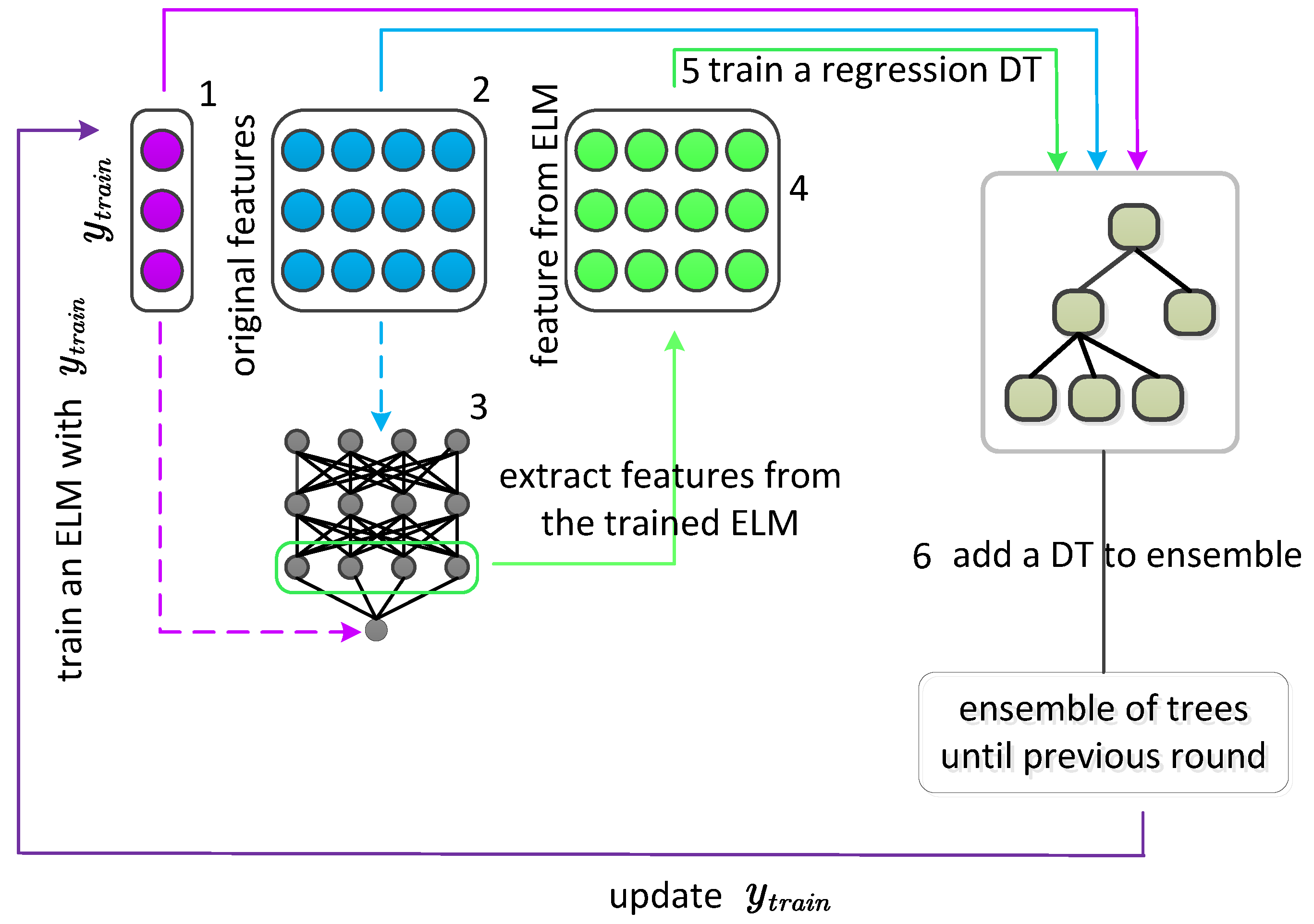
Figure 1 shows the training process of AugBoost-ELM. As shown in Figure 1, the same as the training pattern of classical GBDT, original features are considered as the input of the base regression DTs. In the training process of AugBoost-ELM, before training a new DT to the further ensemble model, each original feature is augmented by a fast neural network-ELM, and the augmented features and the original features are combined as the input of each base learner. By doing this, different from the input of each DT in the original GBDT, the input of each DT of AugBoost-ELM is diversified, thus leading to the base learners of AugBoost-ELM being more diversified and driving the ensemble models to make diversified prediction results. The training pseudo-code of AugBoost-ELM is shown in Algorithm 1.
| Algorithm 1 Pseudo code of AugBoost-ELM |
|
3. Experimental Settings
3.1. Credit Datasets
Australian credit approval dataset is a collection that classifies potential borrowers who may get qualified in getting loans or not by analyzing multiple descriptive attributes range from loan characters, the information of borrowers.
German credit dataset records 1000 credit information from a German bank, each of which contains 20 features. These features include account balance information, duration of credit in a month to repayment history, etc.
Japanese credit dataset contains samples of credit individuals that provide positive or negative credit for banks and lending companies to determine whether granting a loan or not by introducing the knowledge of experts from a Japanese lending institution.
Taiwan dataset is designed to evaluate the predictive performance of the probability of default (PD). This dataset records the credit repayment status of credit card customers in Taiwan since 2005. Through the analysis of this data set, the analysis of credit card customers’ default in mainland China can be used for reference.
3.2. Credit Scoring Benchmark Models
In this study, various credit scoring models are selected as baselines to evaluate the effectiveness of AugBoost-ELM, which includes standard statistical credit scoring methods, ML-based individual classifiers, ensemble approaches. LR and LDA are two representative statistical-based credit scoring models, which have been popularized by researchers, banks, and lending companies due to their simplicity and low implementation advantages.
DT is a tree-structure learning algorithm that realizes credit scoring based on node splitting and tree growth, which have been widely used due to its good training efficiency and interpretability. SVM is a nonlinear learning method that maps a lower-dimensional feature space into a higher-dimensional feature space. KNN implement PD modeling by searching k nearest neighbors as prediction results. NN is a popular approach that is stacked by multiple neural layers to realized hierarchical end-to-end credit scoring. Random forest is an ensemble method that is ensemble by multiple DTs and implements parallel training to enhance the training efficiency of the ensemble framework. GBDT is a boosting-type ensemble solution that improves the predictive performance by iterative optimize the credit scoring error with multiple addictive regression DTs. XGBoost is a more efficient GBDT that grows each DT in a level-wise way. Based on the advantage of gradient descent, LightGBM further improves the training efficiency by leaf-wise growing DTs and introducing exclusive feature bunding (EFB) strategy and gradient-based one-side sampling (GOSS) skill.
3.3. Implementation Details of AugBoost-ELM
The parameters used in AugBoost-ELM can be seen in Table 2. In the implementation of AugBoost-ELM, we use grid search optimization to fine-tune the hyper-parameters in AugBoost-ELM. Since AugBoost-ELM is a variant of GBDT, instead of jointly optimize the number of DTs in AugBoost-ELM and the learning rate, we fix the number of iterations and focus on fine-tuning an appropriate learning rate by a bisection method, the optimal learning rate is further determined by a grid search. Next, we focus on the optimization of hyper-parameters in each DT of AugBoost-ELM. Maximum depth is a parameter that controls the complexity of each DT in AugBoost-ELM, well control of the maximum depth of each DT can avoid the overfitting of AugBoost-ELM. Therefore, we grid search the maximum depth of DTs in AugBoost-ELM from the initialized searching space . Further, we jointly optimize the parameter of minimal samples to split at each splitting node and the parameter of minimal samples at each leaf node from the searching space . The subsample is a hyper-parameter that performs an under-sample operation on the original training set, we search this parameter from the initialized space with fine-tuning stride . In AugBoost-ELM, ELM is performed as a feature augmentation function for GBDT framework, therefore, we further fine-tune the hyper-parameters in ELM to generate robust augmented features. In ELM, the most important parameter that needs to be fine-tuned is the number of hidden nodes L, we search the optimal L from the value set . Since each ELM completes the feature augmentation process in an NN-based framework, a standard feature normalization is first performed on credit data to accelerate the training of the ELM.
3.4. Finetuning Process of Credit Scoring Benchmarks
LR is a simple and linear algorithm that has been widely pursued in practical credit scoring for banks and lending institutions. To get a good predictive performance of LR, we adopt Newton’s method to iteratively minimize the empirical credit scoring error, and penalty is further introduced to alleviate the overfitting problem, which is optimized from the value set of .
KNN is a classical machine learning method that achieves credit scoring by finding the K nearest samples. Its final predictions are averaged from the states of the searched k nearest samples. Therefore, we focus on finetuning this parameter from the interval of with a search stride of 1.
To accelerate the finetuning process of SVM, in this study, radial basis function (RBF) kernel-based SVM is employed in this work for credit scoring. The major hyper-parameters that need to be finetuned in a RBF kernel-based SVM are and C, where regulates the form of mapping space and C represents penalty coefficient, which quantifies the penalty degree of misclassified samples.
We pre-fix the entire structure with two hidden layers to implement NN. We begin by constructing a stable NN structure from the architectural set with 64, 128, and 256 hidden nodes for hidden layers. Following that, we optimize the learning rate based on an initialized searching space of . To finetune the learning rate, we first select an acceptable learning rate interval using dichotomy and then identify the ideal learning rate using grid search with 5-fold cross-validation from the preset learning rate interval. Each hidden layer is activated by a ReLU function, and a sigmoid activation function is followed to get the probabilistic predictions. Because the credit scoring process is modeled as a binary classification process, the weight parameters of the NN are optimized using a binary cross-entropy loss function. Additionally, dropout is employed to minimize overfitting, and the optimal dropout rate is searched from the range of with an optimization step of 0.1.
RF is an efficient approach that realizes credit scoring in a Bagging-ensemble way. In the finetuning of a RF, we first searched the parameter that denotes the number of DTs to ensemble a RF from the interval of with a search step 100. After determining the overall ensemble framework of RF, we further finetune the parameters in each DT. To encourage the diversity of the ensemble, RF allows each tree within it to grow a deep structure to accommodate high bias low variance predictions. we first finetune the maximum depth of each DT in RF from the interval of with a finetune step of 1, where denotes a DT can grow its structure with an arbitrary depth. Next, the parameters of the minimum samples to split at each splitting node and minimum samples at each leaf node are determined by searching from the initial interval with an optimization step of 10.
Different from RF, GBDT ensemble DTs in a boosting ensemble style. Therefore, we first jointly optimize the number of DTs in a GBDT from the initial interval [50, 150] and the learning rate optimized from the initial set . Next, we determine the maximum depth of each DT by searching from the interval of with a search step of 1. Further, the parameters of minimum samples to split at each splitting node and the minimum samples at each leaf node are both determined from with a search step of 10. To further enhance the predictive performance of credit scoring, subsample skill is further incorporated, which is optimized from the set with an optimization step 0.05.
Based on finetuning pattern of GBDT, in the implementation of GBDT, we introduce and regularization into XGBoost framework to alleviate the overfitting issue, both of which are optimized from the initial set . Moreover, to further get a better credit scoring result, data-level subsample and feature-level subsample operations are further introduced, which are finetuned from .
Since AugBoost-ELM is an efficient supervised AugBoost variant, the optimization process of AugBoost-based models can be referred to the implementation details of AugBoost-ELM.
4. Experimental Results
To test the effectiveness of AugBoost-ELM, we first visualize the ROC curves of credit scoring models for comparison. ROC curve, also known as receiver operating characteristic curve, is a graphical measurement that reflects the sensitivity and specificity of credit scoring models under the different thresholds of predictive probability. The x-axis represents the value of false positive rate (FPR) and the y-axis is the value of true positive rate (TPR), where TPR can be calculated as:
FPR is defined as:
In Equations (13) and (14), the prediction results can be classified into four groups: TP, FP, TN, FN, which can be viewed from Table 3.
Where TP is the number of accurate classified samples whose label is “bad”; FP counts the number of samples that are labeled as “good” while the prediction results are “bad”; FN calculates the number of samples whose label is “bad” and predicted as “good”; TN represents the number of “good” applicants that are correctly classified. The larger the area under the ROC curve implies the better performance a credit scoring algorithm is.
To testify the effectiveness of the feature enhancement mechanism for boosting framework, some baseline models are first selected for preliminary study. These models include statistical-based algorithms such as LR and LDA, ML-based individual classifiers such as DT, KNN, SVM, and NN, bagging-type ensemble method RF and boosting-class ensemble approach GBDT.
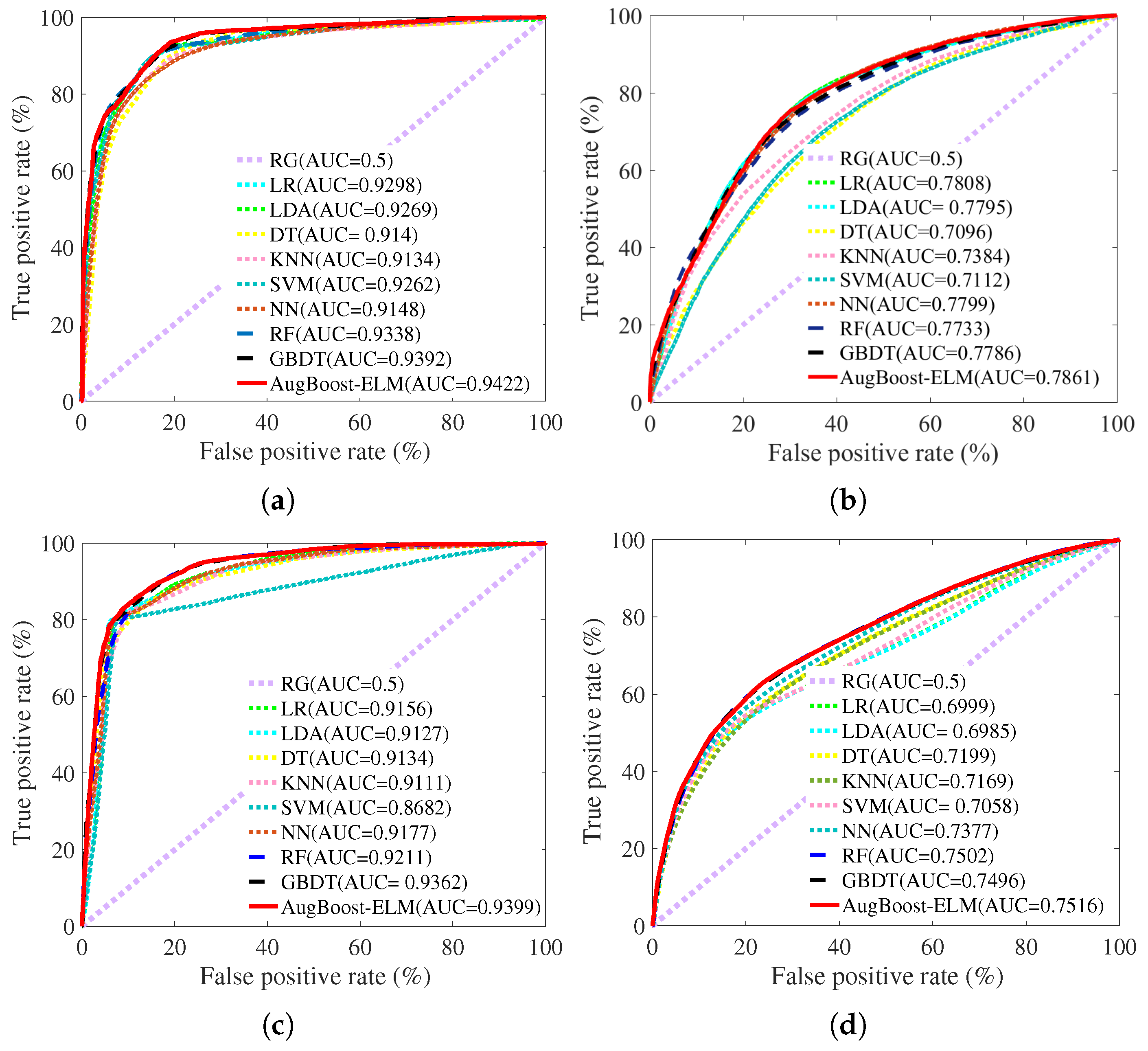
Figure 2 shows the ROC curves of various credit scoring models on the credit datasets. Figure 2a represents the ROC curves of credit scoring models for the Australian dataset; Figure 2b is the ROC curves of credit scoring models for the German dataset; Figure 2c denotes the ROC curves of credit scoring models for the Japanese dataset; Figure 2d illustrates the ROC curves of credit scoring models for the Taiwan dataset. All the ROC curves are an average based on 50 times repeated 10-fold cross-validation.
As is shown in Figure 2a, on the Australian dataset, LR and LDA, KNN gets the smallest area under the ROC curve while AugBoost-ELM gets the largest area under the ROC curve, which demonstrates that AugBoost-ELM is the best algorithm to predict the PD for Australian compared with other baseline models. Compared with KNN, though DT improves the predictive performance, its ROC curve is worse than those of other credit scoring models, indicating that the single DT is not a good solution for accurate credit scoring. Compared with ML-based credit scoring models, statistical-based algorithms LR and LDA get the larger areas under ROC curves, providing evidence that why LR and LDA are popularized by industrial application. Compared with ML-based individual classifiers, the areas under ROC curves of RF and GBDT are significantly larger, which suggests that ensemble multiple weak learners into a stronger one is a good strategy to improve the performance of credit scoring.
As can be viewed from Figure 2c, on the Japanese dataset, the largest area under the ROC curve of AugBoost-ELM implies AugBoost-ELM is the best algorithm for the credit scoring of the Japanese dataset. In addition, SVM gets the smallest area under the ROC curve. Though the ROC curves of other ML-based credit scoring algorithms such as DT, KNN, NN show better predictive ability than SVM, their performance on predicting the PD is worse than that of ensemble learning approaches.
The same as the results on the previous credit datasets, ensemble credit scoring algorithms get a larger ROC curve area compared with other credit scoring models further proves ensemble learning approaches are the good choice to improve the performance of credit scoring. On the Taiwan dataset, as can be observed from Figure 2d, the ROC curve of AugBoost-ELM is close to that of GBDT. To reveal the concrete performance of credit scoring models, we further investigate the quantitative evaluation results of various credit scoring models on the credit datasets. In this study, we selected six metrics to comprehensively compare the performance of the credit scoring model, which include accuracy score, AUC score, precision score, recall score, F1 score, Brier loss.
Accuracy score computes the ratio of samples that are correctly classified, which is defined as:
AUC score calculates the area under the ROC curve and measures the overall predictive performance of credit scoring models.
The precision score represents the ratio of samples whose predicted result is “bad” while its label is “bad”, which can be calculated as:
Recall score measures how many “bad” applicants are correctly predicted, which can be defined as:
F1 is a comprehensive metric of precision score and recall score, which can be calculated as:
Brier loss score describes the average error between the predicted result and the label, which can be calculated as:
where represents the predicted probability of the i-th sample, is the label of the i-th sample, and N is the number of samples.
Table 4 presents the performance comparison of credit scoring models for the Australian dataset. As can be seen from Table 4, AugBoost-ELM gets the best AUC, which is consistent with the ROC curves in Figure 2a, demonstrating AugBoost-ELM is a good choice to recognize good and bad applicants. On the Australian dataset, LR performs well, it achieves the best accuracy score. Therefore, if we are aiming at finding an efficient and effective credit scoring model for the Australian dataset, LR is the best choice. KNN gets the best precision score and worst recall score, leading to the comprehensive performance on the AUC score, F1 score, and BS poor. Moreover, compared with ML-based individual classifiers, RF and GBDT get better AUC score, F1 score, and BS, indicating the effectiveness of ensemble strategy. Compared with GBDT, though AugBoost-ELM gets better AUC score and precision score, its poor recall score results in a small F1 and large BS. In other words, if we focus on the discrimination of good/bad applicants, LR is the best choice; if we are concerned more about the prediction of the PD, AugBoost-ELM is a better choice.
Table 5 shows the performance comparison of credit scoring models for the German dataset. As can be seen from Table 5, AugBoost-ELM gets the optimal AUC score, F1 score, and BS score, revealing that ELM-based supervised feature augmentation is able to enhance the discrimination ability of good/bad applicants. Furthermore, Table 5 further demonstrates statistical-based credit scoring models are the alternative solution to achieve accurate credit scoring compared with ML-based individual classifiers. Furthermore, as is shown in Table 5, in the comparison among ML-based individual classifiers, NN outperforms other ML-based credit scoring algorithms such as DT, KNN, and SVM. This is because NN is a robust algorithm that can learn nonlinear relationships from complex credit datasets. Compared with the bagging-based ensemble method RF, the superior performance of GBDT shows that boosting ensemble strategy is more suitable for the modeling of PD. Based on the good advantage of boosting framework, AugBoost-ELM, which is stage-wisely enhanced by the ELM-based supervised feature augmentation mechanism for the boosting framework, gets better predictive performance.
Table 6 is the performance comparison of credit scoring models for the Japanese dataset. As is shown in Table 6, AugBoost-ELM achieves optimal accuracy score, AUC score, F1 score, and BS while LDA gets the best precision score and GBDT gets the optimal recall score. LDA gets a high precision score and low recall score, suggesting that LDA is a good method to discriminate the good applicant despite the ability to predict the bad applicants is poor. Moreover, compared with statistical-based algorithms and ML-based individual classifiers, the leading performance of RF, GBDT, and AugBoost-ELM further shows that ensemble strategy is practicable for the performance improvement for credit scoring.
Table 7 provides the performance comparison of credit scoring models for the Taiwan dataset. As can be seen from Table 7, AugBoost-ELM realizes optimal scores on the metrics of accuracy, AUC, recall, F1, and BS, the effectiveness of AugBoost-ELM is fully illustrated. The improvement of recall score of AugBoost-ELM specifies the results that AugBoost-ELM improves the performance of credit scoring by reducing the misclassification of “bad” applicants. Moreover, as can be seen from Table 7, ML-based individual classifiers outperform statistical-based algorithms on the Taiwan dataset. Though RF gets a high precision score, its recall score poor ability on discriminating “bad” applicants results in the poor performance of credit scoring for the Taiwan dataset. Besides, the leading performance of AugBoost-ELM compared with GBDT further demonstrates ELM-based supervised features augmentation can be a candidate for the improvement of boosting framework.
To further verify the effectiveness of AugBoost-ELM, we further select five advanced ensemble credit scoring models for comparison, which includes XGBoost, LightGBM, AugBoost-RP, AugBoost-PCA, AugBoost-NN while AugBoost-RP is step-wisely augmented by random projection method, AugBoost-PCA is step-wisely enhanced by principal component analysis (PCA), and AugBoost-NN is enhanced by NN algorithm. Figure 3 shows the testing AUC curves of advanced ensemble credit scoring algorithms. Figure 3a is the testing curves of advanced ensemble methods for the Australian dataset; Figure 3b represents the testing curves of advanced ensemble algorithms for the German dataset; Figure 3c illustrates the testing curves of advanced ensemble approaches for the Japanese dataset; Figure 3d provides the testing curves of advanced ensemble methods for the Taiwan dataset.
As can be seen from Figure 3a, the converged testing AUC curve of AugBoost-ELM is close to that of AugBoost-NN, both of which are higher than the converged testing AUC of unsupervised AugBoost-based models such as AugBoost-RP and AugBoost-PCA. Moreover, as can be seen from Figure 3a, AugBoost-based models are superior to advanced ensemble approaches such as XGBoost and LightGBM. As can be observed from Figure 3b, AugBoost-ELM gets the highest converged testing AUC than other advanced ensemble approaches. Compared with unsupervised AugBoost-based models, XGBoost and LightGBM achieve better testing AUC while their converged testing AUC is worse than that of supervised AugBoost-based models; Compared with AugBoost-NN, AugBoost-ELM gets a slightly higher testing AUC than AugBoost-NN, demonstrating that AugBoost-ELM can be a good alternative to AugBoost-NN. As can be viewed from Figure 3c, similar to the results in Figure 3b, the testing AUC curve of AugBoost-ELM is slightly higher than that of another supervised enhanced GBDT model AugBoost-NN; AugBoost-based models get higher converged testing curves of advanced ensemble approaches. The same conclusion can be drawn from Figure 3d for the Taiwan dataset.
Table 8 shows the performance comparison of advanced ensemble models for credit datasets. As can be seen from Table 8, on the Australian dataset, AugBoost-NN gets the best values of the metrics of AUC, recall, and F1 while AugBoost-PCA gets the optimal accuracy score and precision score. Compared with advanced ensemble approaches such as XGBoost, LightGBM, AugBoost-RP, and AugBoost-PCA, AugBoost-ELM achieves comparable performance on the AUC score, F1 score, demonstrating that AugBoost-ELM can be an alternative supervised AugBoost model to AugBoost-NN. On the German dataset, Japanese dataset, and Taiwan dataset, AugBoost-ELM get the best values of accuracy score, AUC score, recall score, F1 score, and BS, demonstrating that AugBoost-ELM is a comparable approach to other advanced ensemble approaches such as XGBoost, LightGBM, AugBoost-RP, AugBoost-PCA, and AugBoost-NN.
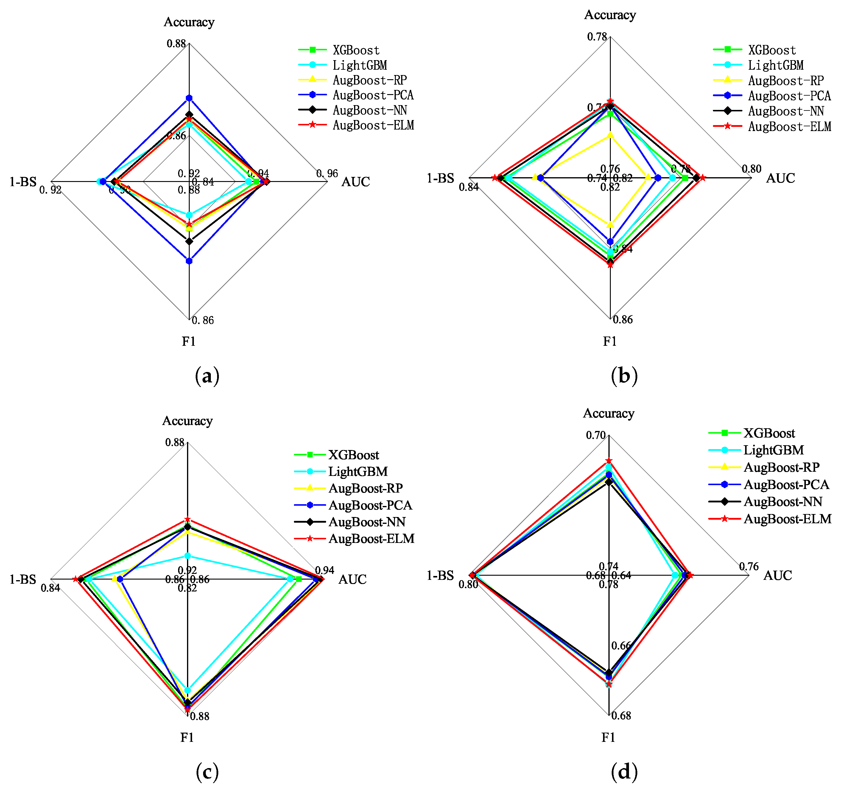
To analyze the overall performance of credit scoring, we select four comprehensive evaluation metrics, which include accuracy score, AUC score, F1 score, and BS for the further comparison. Figure 4 shows the radar maps of advanced ensemble models for the credit datasets. Figure 4a is the comparison result of ensemble approaches for the Australian dataset; Figure 4b represents the performance radar map of advanced ensemble approaches for the German dataset; Figure 4c illustrates the performance radar map of advanced ensemble methods for the Japanese dataset; Figure 4a provides the performance radar map of advanced ensemble algorithms for the Taiwan dataset. The larger area that one radar map covers, the better overall performance a credit scoring model implies.
As can be seen from Figure 4a, on the Australian dataset, AugBoost-ELM outperforms XGBoost and LightGBM while its radar map area is smaller than that of the other three AugBoost-based models including AugBoost-RP, AugBoost-PCA, and AugBoost-NN. As is shown in Figure 4b–d, on the German dataset, Japanese dataset, and Taiwan dataset, AugBoost-ELM gets the largest radar maps area than other advanced boosting-based ensemble algorithms, not only providing the evidence that the supervised ELM-based feature augmentation can be an alternative to NN-based feature augmentation for boosting framework but also giving the illustration that supervised feature augmentation skill is superior to unsupervised feature augmentation for GBDT.
Since each credit scoring metric has its advantages and limitations, to give a view of the statistical ranks for credit scoring models, we perform a significance test procedure. Because parametric significance test method computers statistic value based on the assumption that credit scoring datasets follow a normal distribution, we adopt a simple and powerful non-parametric way for significance test. In this study, Friedman test, a rank-based non-parametric significance test, is introduced to investigate the statistical performance of credit scoring algorithms. The Friedman statistic value is calculated as:
where K denotes the number of classifiers, D represents the number of datasets. is the average rank of k-th classifier, and , , , , are the ranks of k-th classifier on d-th dataset that are computed based on accuracy score, AUC, F1, and BS, respectively. By calculating the Friedman statistic value, the issue of whether there is a significant difference among credit scoring models is detected. Specifically, when is larger than a critical value at a significance level, the null hypothesis (there is no significant difference between credit scoring models) is rejected, and a post hoc test, Nemenyi test, is further performed for pair-wise comparison. The critical difference () can be defined as:
where is the critical difference at significance level , is the critical value at significance level , which is computed from a studentized range.
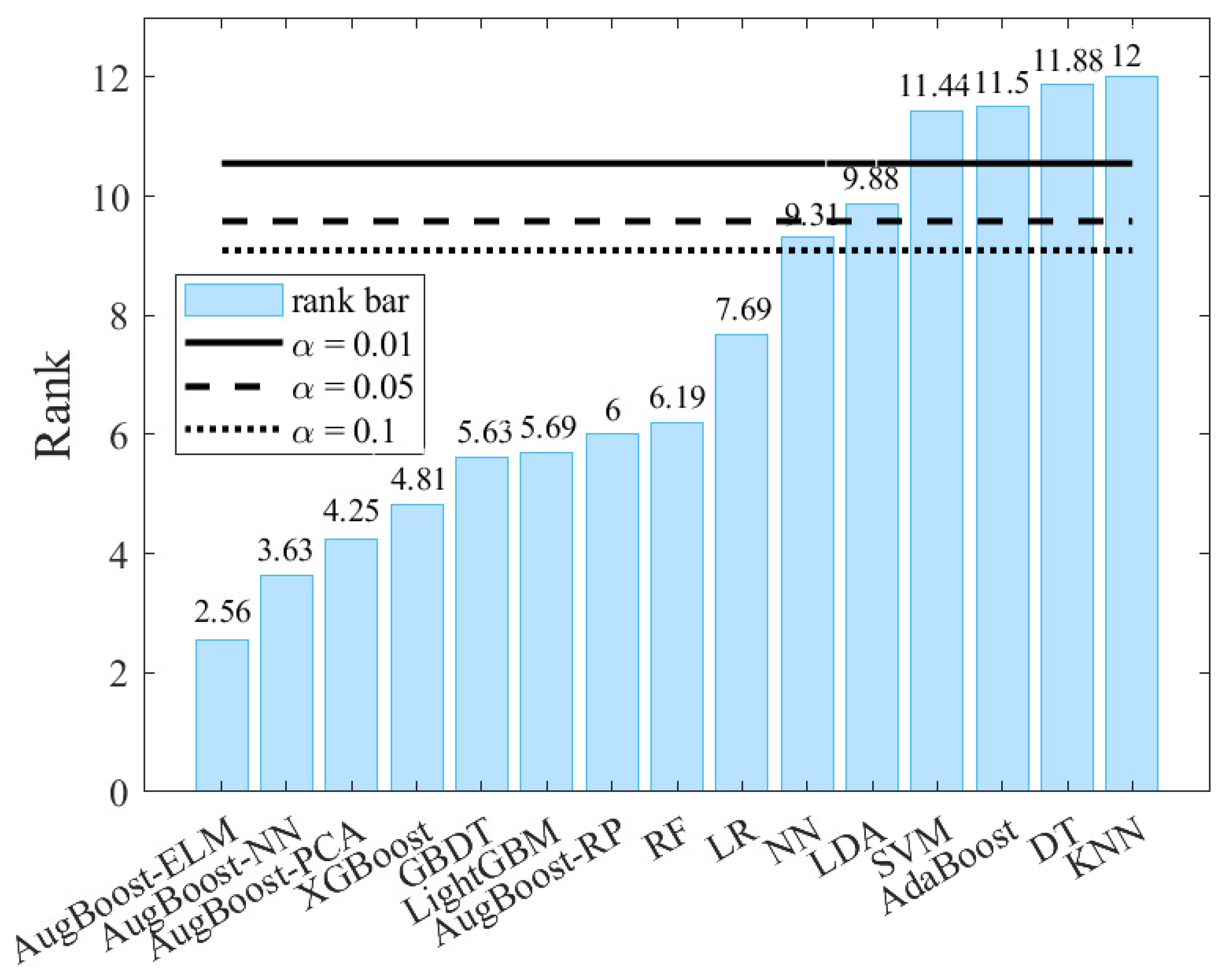
To investigate the statistical difference among credit scoring models, we first compute according to Equation (20), rejecting the null hypothesis at significance level . Next, we perform Nemenyi test for pair-wise comparison. , , are first calculated to further computed CDs for different significance levels. According to Equation (21), we can get , , .
Figure 5 shows the average ranks of credit scoring models for the Nemenyi test. As can be seen from Figure 5, if we consider AugBoost-ELM as the comparison baseline, SVM, AdaBoost, DT, and KNN are statistically inferior to AugBoost at significance level ; moreover, AugBoost-ELM outperforms LDA at the significance level as well as it is superior to NN at the significance level . Besides, as illustrated in Figure 5, AugBoost-ELM, AugBoost-NN, and AugBoost-PCA rank in top 3, demonstrating the effectiveness of the augmentation mechanism for GBDT framework. The lower ranks of AugBoost-ELM and AugBoost-NN compared with AugBoost-PCA and AugBoost-RP further verify supervised augmentation is a better augmentation compared with unsupervised feature augmentation for GBDT.
In this study, ELM accomplishes the supervised step-wise feature augmentation process for GBDT, which avoids the iterative error back-propagation process of NN. Compared with NN-based feature augmentation for GBDT, ELM-based supervised feature augmentation accelerates the training process of the GBDT-based framework and avoids falling into local minima, leading to the robust generation of augmented features. Based on the above analysis, we further investigate the training efficiency by comparing the training cost of AugBoost-based models on the four credit datasets. Table 9 shows the training cost comparison of AugBoost-based models on the four credit datasets. As can be seen from Table 9, unsupervised AugBoost-based models such as AugBoost-RP and AugBoost-PCA get faster training speed. However, combined with the performance comparison analyzed above, supervised AugBoost models are the better solution for accurate credit scoring. Besides, as can be seen from the efficiency comparison among AugBoost-NN and AugBoost-ELM, the training efficiency of AugBoost-ELM has been greatly improved. Compared with AugBoost-NN, AugBoost-ELM reduces the training time by 86.90%, 85.24%, 88.14%, and 98.58% for the Australian dataset, German dataset, Japan dataset, and Taiwan dataset, respectively. Even in the incorporation with 1080Ti GPU, compared with AugBoost-NN, the efficiency improvement of AugBoost-ELM on large-scale datasets such as Taiwan is more significant than that on the small-scale datasets such as Australian, German, and Japan.
5. Conclusions
In this study, a supervised NN-based augmented GBDT-AugBoost-ELM is proposed to improve the performance of credit scoring. AugBoost-ELM is a variant of GBDT, which is step-wisely enhanced by the extreme learning machine to enhance the diversity of DTs in GBDT. ELM-based feature augmentation process not only provides robust augmented feature generation but also improves the efficiency of the feature augmentation process for GBDT compared with NN-based feature augmentation. The experimental results on four credit datasets show that AugBoost-ELM is an effective GBDT to improve the performance of credit scoring. Compared with NN-based feature supervised feature augmentation, ELM-based feature augmentation is not only beneficial to the performance of the boosting framework but also provides a way to accelerate the training process of supervised augmented GBDT.
Though AugBoost-ELM improves the performance of credit scoring and provides an efficient way to augment features for the GBDT framework, there are some issues that need to be further tackled: (1) in this study, the NN architecture and ELM framework are optimized via grid search method, future work will focus on introducing some advanced hyper-parameters optimization algorithms such as Bayesian optimization method [46,47], and evolutionary optimization strategies [48]. (2) The research of ML-based credit scoring is gradually marching towards the direction of large-scale credit scoring, in future work, some larger-scale datasets will be collected to further testify the effectiveness of AugBoost-ELM. (3) Classical GBDT is an inefficient training framework compared with XGBoost and LightGBM. Consequently, some efficient supervised and unsupervised feature augmentation methods are considered into the XGBoost and LightGBM [49] to further enhance the performance and improve the efficiency of credit scoring.
Author Contributions
Conceptualization and supervision, C.G.; Investigation, Methodology, validation, writing-original draft, Y.Z.; writing-review & editing, C.G. and Y.Z. All authors have read and agreed to the published version of the manuscript.
Funding
This work was supported in part by the National Natural Science Foundation of China (71874027), in part by the Shanghai Planning Office of Philosophy and Social Science (2021ECK001), and in part by the Shanghai Sailing Program (21YF1415900).
Institutional Review Board Statement
Not applicable.
Informed Consent Statement
Not applicable.
Data Availability Statement
Not applicable.
Conflicts of Interest
The authors declare no conflict of interest.
References
- Simumba, N.; Okami, S.; Kodaka, A.; Kohtake, N. Comparison of Profit-Based Multi-Objective Approaches for Feature Selection in Credit Scoring. Algorithms 2021, 14, 260. [Google Scholar] [CrossRef]
- Almhaithawi, D.; Jafar, A.; Aljnidi, M. Example-dependent cost-sensitive credit cards fraud detection using SMOTE and Bayes minimum risk. SN Appl. Sci. 2020, 2, 1–12. [Google Scholar]
- Pang, S.; Hou, X.; Xia, L. Borrowers’ credit quality scoring model and applications, with default discriminant analysis based on the extreme learning machine. Technol. Forecast. Soc. Chang. 2021, 165, 120462. [Google Scholar] [CrossRef]
- Mahmoudi, N.; Duman, E. Detecting credit card fraud by modified Fisher discriminant analysis. Expert Syst. Appl. 2015, 42, 2510–2516. [Google Scholar] [CrossRef]
- Sohn, S.Y.; Kim, D.H.; Yoon, J.H. Technology credit scoring model with fuzzy logistic regression. Appl. Soft Comput. 2016, 43, 150–158. [Google Scholar] [CrossRef]
- Dumitrescu, E.; Hue, S.; Hurlin, C.; Tokpavi, S. Machine learning for credit scoring: Improving logistic regression with non-linear decision-tree effects. Eur. J. Oper. Res. 2022, 22, 1178–1192. [Google Scholar] [CrossRef]
- Luo, C.; Wu, D.; Wu, D. A deep learning approach for credit scoring using credit default swaps. Eng. Appl. Artif. Intell. 2017, 65, 465–470. [Google Scholar] [CrossRef]
- Zhao, Z.; Xu, S.; Kang, B.H.; Kabir, M.M.J.; Liu, Y.; Wasinger, R. Investigation and improvement of multi-layer perceptron neural networks for credit scoring. Expert Syst. Appl. 2015, 42, 3508–3516. [Google Scholar] [CrossRef]
- Xia, Y.; Zhao, J.; He, L.; Li, Y.; Niu, M. A novel tree-based dynamic heterogeneous ensemble method for credit scoring. Expert Syst. Appl. 2020, 159, 113615. [Google Scholar] [CrossRef]
- Şen, D.; Dönmez, C.Ç.; Yıldırım, U.M. A hybrid bi-level metaheuristic for credit scoring. Inf. Syst. Front. 2020, 22, 1009–1019. [Google Scholar] [CrossRef]
- Harris, T. Credit scoring using the clustered support vector machine. Expert Syst. Appl. 2015, 42, 741–750. [Google Scholar] [CrossRef] [Green Version]
- Abdelmoula, A.K. Bank credit risk analysis with k-nearest-neighbor classifier: Case of Tunisian banks. Account. Manag. Inf. Syst. 2015, 14, 79. [Google Scholar]
- Pławiak, P.; Abdar, M.; Pławiak, J.; Makarenkov, V.; Acharya, U.R. DGHNL: A new deep genetic hierarchical network of learners for prediction of credit scoring. Inf. Sci. 2020, 516, 401–418. [Google Scholar] [CrossRef]
- Hu, Y.C.; Ansell, J. Measuring retail company performance using credit scoring techniques. Eur. J. Oper. Res. 2007, 183, 1595–1606. [Google Scholar] [CrossRef]
- Okesola, O.J.; Okokpujie, K.O.; Adewale, A.A.; John, S.N.; Omoruyi, O. An improved bank credit scoring model: A naïve Bayesian approach. In Proceedings of the 2017 International Conference on Computational Science and Computational Intelligence (CSCI), Las Vegas, NV, USA, 14–16 December 2017; pp. 228–233. [Google Scholar]
- Liu, W.; Fan, H.; Xia, M. Step-wise multi-grained augmented gradient boosting decision trees for credit scoring. Eng. Appl. Artif. Intell. 2021, 97, 104036. [Google Scholar] [CrossRef]
- Koutanaei, F.N.; Sajedi, H.; Khanbabaei, M. A hybrid data mining model of feature selection algorithms and ensemble learning classifiers for credit scoring. J. Retail. Consum. Serv. 2015, 27, 11–23. [Google Scholar] [CrossRef]
- Nikolic, N.; Zarkic-Joksimovic, N.; Stojanovski, D.; Joksimovic, I. The application of brute force logistic regression to corporate credit scoring models: Evidence from Serbian financial statements. Expert Syst. Appl. 2013, 40, 5932–5944. [Google Scholar] [CrossRef]
- Eisenbeis, R.A. Problems in applying discriminant analysis in credit scoring models. J. Bank. Financ. 1978, 2, 205–219. [Google Scholar] [CrossRef]
- Nai, W.; Liu, L.; Wang, S.; Dong, D. Modeling the trend of credit card usage behavior for different age groups based on singular spectrum analysis. Algorithms 2018, 11, 15. [Google Scholar] [CrossRef] [Green Version]
- Devi, C.D.; Chezian, R.M. A relative evaluation of the performance of ensemble learning in credit scoring. In Proceedings of the 2016 IEEE International Conference on Advances in Computer Applications (ICACA), Coimbatore, India, 24 October 2016; pp. 161–165. [Google Scholar]
- Li, Z.; Tian, Y.; Li, K.; Zhou, F.; Yang, W. Reject inference in credit scoring using semi-supervised support vector machines. Expert Syst. Appl. 2017, 74, 105–114. [Google Scholar] [CrossRef]
- Tsai, C.F.; Wu, J.W. Using neural network ensembles for bankruptcy prediction and credit scoring. Expert Syst. Appl. 2008, 34, 2639–2649. [Google Scholar] [CrossRef]
- Lee, T.S.; Chiu, C.C.; Chou, Y.C.; Lu, C.J. Mining the customer credit using classification and regression tree and multivariate adaptive regression splines. Comput. Stat. Data Anal. 2006, 50, 1113–1130. [Google Scholar] [CrossRef]
- Dohmatob, E. Generalized no free lunch theorem for adversarial robustness. In Proceedings of the International Conference on Machine Learning, Long Beach, CA, USA, 9–15 June 2019; pp. 1646–1654. [Google Scholar]
- Pławiak, P.; Abdar, M.; Acharya, U.R. Application of new deep genetic cascade ensemble of SVM classifiers to predict the Australian credit scoring. Appl. Soft Comput. 2019, 84, 105740. [Google Scholar] [CrossRef]
- Abellán, J.; Castellano, J.G. A comparative study on base classifiers in ensemble methods for credit scoring. Expert Syst. Appl. 2017, 73, 1–10. [Google Scholar] [CrossRef]
- Ala’raj, M.; Abbod, M.F. A new hybrid ensemble credit scoring model based on classifiers consensus system approach. Expert Syst. Appl. 2016, 64, 36–55. [Google Scholar] [CrossRef]
- Zhang, W.; Yang, D.; Zhang, S.; Ablanedo-Rosas, J.H.; Wu, X.; Lou, Y. A novel multi-stage ensemble model with enhanced outlier adaptation for credit scoring. Expert Syst. Appl. 2021, 165, 113872. [Google Scholar] [CrossRef]
- Feng, X.; Xiao, Z.; Zhong, B.; Qiu, J.; Dong, Y. Dynamic ensemble classification for credit scoring using soft probability. Appl. Soft Comput. 2018, 65, 139–151. [Google Scholar] [CrossRef]
- Zhang, W.; Yang, D.; Zhang, S. A new hybrid ensemble model with voting-based outlier detection and balanced sampling for credit scoring. Expert Syst. Appl. 2021, 174, 114744. [Google Scholar] [CrossRef]
- Xia, Y.; Liu, C.; Da, B.; Xie, F. A novel heterogeneous ensemble credit scoring model based on bstacking approach. Expert Syst. Appl. 2018, 93, 182–199. [Google Scholar] [CrossRef]
- Nalić, J.; Martinović, G.; Žagar, D. New hybrid data mining model for credit scoring based on feature selection algorithm and ensemble classifiers. Adv. Eng. Inform. 2020, 45, 101130. [Google Scholar] [CrossRef]
- Louzada, F.; Anacleto-Junior, O.; Candolo, C.; Mazucheli, J. Poly-bagging predictors for classification modelling for credit scoring. Expert Syst. Appl. 2011, 38, 12717–12720. [Google Scholar] [CrossRef]
- He, H.; Zhang, W.; Zhang, S. A novel ensemble method for credit scoring: Adaption of different imbalance ratios. Expert Syst. Appl. 2018, 98, 105–117. [Google Scholar] [CrossRef]
- Zhang, X.; Yang, Y.; Zhou, Z. A novel credit scoring model based on optimized random forest. In Proceedings of the 2018 IEEE 8th Annual Computing and Communication Workshop and Conference (CCWC), Las Vegas, NV, USA, 8–10 January 2018; pp. 60–65. [Google Scholar]
- Liu, W.; Fan, H.; Xia, M. Multi-grained and multi-layered gradient boosting decision tree for credit scoring. Appl. Intell. 2021, 52, 5325–5341. [Google Scholar] [CrossRef]
- Sohn, S.Y.; Kim, J.W. Decision tree-based technology credit scoring for start-up firms: Korean case. Expert Syst. Appl. 2012, 39, 4007–4012. [Google Scholar] [CrossRef]
- Xia, Y.; Liu, C.; Li, Y.; Liu, N. A boosted decision tree approach using Bayesian hyper-parameter optimization for credit scoring. Expert Syst. Appl. 2017, 78, 225–241. [Google Scholar] [CrossRef]
- Tannor, P.; Rokach, L. AugBoost: Gradient Boosting Enhanced with Step-Wise Feature Augmentation. In Proceedings of the IJCAI, Macao, China, 10–16 August 2019; pp. 3555–3561. [Google Scholar]
- Huang, G.B.; Zhu, Q.Y.; Siew, C.K. Extreme learning machine: Theory and applications. Neurocomputing 2006, 70, 489–501. [Google Scholar] [CrossRef]
- Ding, S.; Xu, X.; Nie, R. Extreme learning machine and its applications. Neural Comput. Appl. 2014, 25, 549–556. [Google Scholar] [CrossRef]
- Cannings, T.I.; Samworth, R.J. Random-projection ensemble classification. arXiv 2015, arXiv:1504.04595. [Google Scholar] [CrossRef]
- Liu, W.; Fan, H.; Xia, M. Credit scoring based on tree-enhanced gradient boosting decision trees. Expert Syst. Appl. 2022, 189, 116034. [Google Scholar] [CrossRef]
- Dua, D.; Graff, C. UCI Machine Learning Repository. 2019. Available online: http://archive.ics.uci.edu/ml (accessed on 21 February 2022).
- Feurer, M.; Springenberg, J.; Hutter, F. Initializing bayesian hyperparameter optimization via meta-learning. In Proceedings of the Proceedings of the AAAI Conference on Artificial Intelligence, Austin, TX, USA, 25–30 January 2015; Volume 29. [Google Scholar]
- Yotsawat, W.; Wattuya, P.; Srivihok, A. Improved credit scoring model using XGBoost with Bayesian hyper-parameter optimization. Int. J. Electr. Comput. Eng. 2021, 11, 5477–5487. [Google Scholar] [CrossRef]
- Silva, P.C.; de Lima e Silva, P.C.; Sadaei, H.J.; Guimarães, F.G. Distributed evolutionary hyperparameter optimization for fuzzy time series. IEEE Trans. Netw. Serv. Manag. 2020, 17, 1309–1321. [Google Scholar] [CrossRef]
- Ke, G.; Meng, Q.; Finley, T.; Wang, T.; Chen, W.; Ma, W.; Ye, Q.; Liu, T.Y. Lightgbm: A highly efficient gradient boosting decision tree. Adv. Neural Inf. Process. Syst. 2017, 30, 3146–3154. [Google Scholar]
Figure 1.
Training process of AugBoost-ELM.

Figure 2.
ROCs comparison of benchmark credit scoring models for credit datasets: RG represents the curve of random guess. (a) Australian, (b) German, (c) Japanese, (d) Taiwan.
Figure 2.
ROCs comparison of benchmark credit scoring models for credit datasets: RG represents the curve of random guess. (a) Australian, (b) German, (c) Japanese, (d) Taiwan.

Figure 3.
Comparison of testing AUC for the credit datasets. (a) Australian, (b) German, (c) Japanese, (d) Taiwan.
Figure 3.
Comparison of testing AUC for the credit datasets. (a) Australian, (b) German, (c) Japanese, (d) Taiwan.

Figure 4.
Comparison of testing AUC for the credit datasets. (a) Australian, (b) German, (c) Japanese, (d) Taiwan.
Figure 4.
Comparison of testing AUC for the credit datasets. (a) Australian, (b) German, (c) Japanese, (d) Taiwan.

Figure 5.
Average ranks of credit scoring models for the Nemenyi test: the black solid line is , the dotted line denotes the , and the point line represents .
Figure 5.
Average ranks of credit scoring models for the Nemenyi test: the black solid line is , the dotted line denotes the , and the point line represents .


Table 1.
Information of credit datasets.
| Dataset | Samples | Variables | Good/Bad |
|---|---|---|---|
| Australian | 690 | 14 | 307/383 |
| German | 1000 | 24 | 700/300 |
| Japanese | 690 | 15 | 296/357 |
| Taiwan | 6000 | 23 | 3000/3000 |
Table 2.
Parameters setting of AugBoost-ELM.
| Hyperparameters | Description | Searching Space | Stride |
|---|---|---|---|
| n_estimators | The number of DTs | 100 | / |
| learning_rate | Learning rate that control the optimization step | biSection | |
| max_depth | Maximum depth of DT in each | 1 | |
| min_sample_split | Minimal samples to split at each splitting node | 5 | |
| min_samples_leaf | Minimal samples at each leaf node | 5 | |
| subsample | Undersampling ratio on the training set | ||
| max_features | Maximum candidate features for node splitting | biSection | |
| L | Number of hidden nodes of ELM | / | |
| Period of performing feature augmentation for boosting | / |
Table 3.
Confusion matrix of prediction results.
| Label | |||
|---|---|---|---|
| Bad | Good | ||
| Prediction | Bad | TP | FP |
| Good | FN | TN | |
Table 4.
Performance comparison of credit scoring models for the Australian dataset.
| Algorithm | Accuracy | AUC | Precision | Recall | F1 | BS |
|---|---|---|---|---|---|---|
| LR | 0.8649 | 0.9298 | 0.8309 | 0.8741 | 0.852 | 0.0992 |
| LDA | 0.8594 | 0.9269 | 0.7961 | 0.9196 | 0.8534 | 0.1089 |
| DT | 0.8437 | 0.914 | 0.827 | 0.8202 | 0.8236 | 0.1113 |
| KNN | 0.8494 | 0.9134 | 0.864 | 0.7851 | 0.8227 | 0.1112 |
| SVM | 0.8626 | 0.9262 | 0.8497 | 0.8395 | 0.8446 | 0.1008 |
| NN | 0.8502 | 0.9148 | 0.8328 | 0.8298 | 0.8313 | 0.1186 |
| RF | 0.8645 | 0.9338 | 0.8575 | 0.8341 | 0.8457 | 0.1032 |
| GBDT | 0.8637 | 0.9392 | 0.8426 | 0.853 | 0.8478 | 0.0956 |
| AugBoost-ELM | 0.8635 | 0.9422 | 0.8485 | 0.8439 | 0.8462 | 0.0993 |
Table 5.
Performance comparison of credit scoring models for the German dataset.
| Algorithm | Accuracy | AUC | Precision | Recall | F1 | BS |
|---|---|---|---|---|---|---|
| LR | 0.7601 | 0.7808 | 0.7942 | 0.8872 | 0.8381 | 0.1646 |
| LDA | 0.7585 | 0.7795 | 0.7926 | 0.8871 | 0.8372 | 0.1653 |
| DT | 0.7232 | 0.7096 | 0.7791 | 0.8439 | 0.8102 | 0.1928 |
| KNN | 0.728 | 0.7384 | 0.7341 | 0.9586 | 0.8315 | 0.1803 |
| SVM | 0.7065 | 0.7112 | 0.7966 | 0.7798 | 0.7881 | 0.1859 |
| NN | 0.7659 | 0.7799 | 0.8067 | 0.8753 | 0.8396 | 0.165 |
| RF | 0.747 | 0.7733 | 0.7571 | 0.9407 | 0.839 | 0.17 |
| GBDT | 0.7586 | 0.7786 | 0.788 | 0.8962 | 0.8386 | 0.1655 |
| AugBoost-ELM | 0.7617 | 0.7861 | 0.7775 | 0.9245 | 0.8446 | 0.1637 |
Table 6.
Performance comparison of credit scoring models for the Japanese dataset.
| Algorithm | Accuracy | AUC | Precision | Recall | F1 | BS |
|---|---|---|---|---|---|---|
| LR | 0.8549 | 0.9156 | 0.9175 | 0.8116 | 0.8613 | 0.103 |
| LDA | 0.8606 | 0.9127 | 0.9402 | 0.7997 | 0.8643 | 0.1136 |
| DT | 0.849 | 0.9134 | 0.8698 | 0.8561 | 0.8629 | 0.1123 |
| KNN | 0.8487 | 0.9111 | 0.8862 | 0.8345 | 0.8596 | 0.1107 |
| SVM | 0.8566 | 0.8682 | 0.9312 | 0.8008 | 0.8611 | 0.1175 |
| NN | 0.8487 | 0.9177 | 0.8895 | 0.831 | 0.8593 | 0.1048 |
| RF | 0.8548 | 0.9211 | 0.9293 | 0.7993 | 0.8594 | 0.1509 |
| GBDT | 0.8642 | 0.9362 | 0.8898 | 0.8625 | 0.8759 | 0.096 |
| AugBoost-ELM | 0.8687 | 0.9399 | 0.901 | 0.8582 | 0.8791 | 0.0942 |
Table 7.
Performance comparison of credit scoring models for the Taiwan dataset.
| Algorithm | Accuracy | AUC | Precision | Recall | F1 | BS |
|---|---|---|---|---|---|---|
| LR | 0.6486 | 0.6999 | 0.6612 | 0.6099 | 0.6345 | 0.2179 |
| LDA | 0.6512 | 0.6985 | 0.6676 | 0.6023 | 0.6333 | 0.2183 |
| KNN | 0.6676 | 0.7169 | 0.7164 | 0.555 | 0.6254 | 0.2135 |
| SVM | 0.6731 | 0.7058 | 0.7561 | 0.5114 | 0.6101 | 0.214 |
| NN | 0.6806 | 0.7377 | 0.7131 | 0.6044 | 0.6543 | 0.2061 |
| DT | 0.6666 | 0.7199 | 0.6851 | 0.6167 | 0.6491 | 0.2152 |
| RF | 0.6949 | 0.7502 | 0.7298 | 0.6192 | 0.67 | 0.2011 |
| GBDT | 0.6948 | 0.7496 | 0.7297 | 0.6189 | 0.6698 | 0.2009 |
| AugBoost-ELM | 0.6963 | 0.7516 | 0.7322 | 0.6194 | 0.6711 | 0.2005 |
Table 8.
Performance comparison of advanced ensemble models for credit datasets.
| Dataset | Algorithm | Accuracy | AUC | Precision | Recall | F1 | BS |
|---|---|---|---|---|---|---|---|
| Australian | XGBoost | 0.8633 | 0.9394 | 0.8449 | 0.8487 | 0.8468 | 0.0992 |
| LightGBM | 0.8624 | 0.9371 | 0.8476 | 0.8422 | 0.8449 | 0.0942 | |
| AugBoost-RP | 0.8633 | 0.9416 | 0.8449 | 0.8487 | 0.8468 | 0.0991 | |
| AugBoost-PCA | 0.8681 | 0.9415 | 0.8533 | 0.8497 | 0.8515 | 0.0951 | |
| AugBoost-NN | 0.8645 | 0.9424 | 0.8435 | 0.8539 | 0.8487 | 0.0984 | |
| AugBoost-ELM | 0.8635 | 0.9422 | 0.8485 | 0.8439 | 0.8462 | 0.0993 | |
| German | XGBoost | 0.7582 | 0.7811 | 0.7757 | 0.9208 | 0.842 | 0.1652 |
| LightGBM | 0.7615 | 0.7776 | 0.7887 | 0.9007 | 0.841 | 0.1657 | |
| AugBoost-RP | 0.7519 | 0.7707 | 0.7862 | 0.8867 | 0.8335 | 0.1694 | |
| AugBoost-PCA | 0.7605 | 0.7735 | 0.7956 | 0.8852 | 0.838 | 0.1702 | |
| AugBoost-NN | 0.7604 | 0.7843 | 0.7766 | 0.9237 | 0.8438 | 0.1644 | |
| AugBoost-ELM | 0.7617 | 0.7861 | 0.7775 | 0.9245 | 0.8446 | 0.1637 | |
| Japanese | XGBoost | 0.8678 | 0.9362 | 0.8959 | 0.8625 | 0.8789 | 0.095 |
| LightGBM | 0.8634 | 0.9349 | 0.8829 | 0.8696 | 0.8762 | 0.0957 | |
| AugBoost-RP | 0.8669 | 0.9398 | 0.8964 | 0.8599 | 0.8778 | 0.095 | |
| AugBoost-PCA | 0.8676 | 0.9388 | 0.8957 | 0.8622 | 0.8786 | 0.0949 | |
| AugBoost-NN | 0.8676 | 0.9395 | 0.9004 | 0.8567 | 0.878 | 0.0944 | |
| AugBoost-ELM | 0.8687 | 0.9399 | 0.901 | 0.8582 | 0.8791 | 0.0942 | |
| Taiwan | XGBoost | 0.6945 | 0.7504 | 0.7301 | 0.6175 | 0.6691 | 0.2006 |
| LightGBM | 0.6954 | 0.7494 | 0.7292 | 0.6218 | 0.6712 | 0.201 | |
| AugBoost-RP | 0.6941 | 0.7508 | 0.7295 | 0.617 | 0.6686 | 0.2007 | |
| AugBoost-PCA | 0.6943 | 0.7508 | 0.7297 | 0.6174 | 0.6689 | 0.2006 | |
| AugBoost-NN | 0.6933 | 0.7514 | 0.7285 | 0.616 | 0.6677 | 0.2005 | |
| AugBoost-ELM | 0.6963 | 0.7516 | 0.7322 | 0.6194 | 0.6711 | 0.2005 |
Table 9.
Training cost of various AugBoost-based models on the four credit datasets: all the training costs are averaged over 50 times 10-fold cross-validation, the unit of training cost is second, all the results are run on the experimental environment of CPU Intel 9700K with RAM 32 GB and GPU 1080Ti; our implementation is based on python 3.5, gradient boosting framework are realized based on Scikit-learn 0.19.1, AugBoost-NN (GPU) is accelerated by a 1080Ti GPU, which is implemented and tested in Keras with Tensorflow backend.
| Algorithm | Australian | German | Japanese | Taiwan |
|---|---|---|---|---|
| AugBoost-RP | 0.32 | 1.11 | 0.45 | 3.61 |
| AugBoost-PCA | 1.05 | 1.33 | 0.52 | 3.86 |
| AugBoost-NN | 245.21 | 280.78 | 300.89 | 3673.68 |
| AugBoost-NN (GPU) | 270.34 | 260.12 | 254.33 | 388.49 |
| AugBoost-ELM | 32.12 | 41.45 | 35.66 | 51.94 |
Publisher’s Note: MDPI stays neutral with regard to jurisdictional claims in published maps and institutional affiliations. |
© 2022 by the authors. Licensee MDPI, Basel, Switzerland. This article is an open access article distributed under the terms and conditions of the Creative Commons Attribution (CC BY) license (https://creativecommons.org/licenses/by/4.0/).
Share and Cite
MDPI and ACS Style
Zou, Y.; Gao, C. Extreme Learning Machine Enhanced Gradient Boosting for Credit Scoring. Algorithms 2022, 15, 149. https://0-doi-org.brum.beds.ac.uk/10.3390/a15050149
AMA Style
Zou Y, Gao C. Extreme Learning Machine Enhanced Gradient Boosting for Credit Scoring. Algorithms. 2022; 15(5):149. https://0-doi-org.brum.beds.ac.uk/10.3390/a15050149
Chicago/Turabian StyleZou, Yao, and Changchun Gao. 2022. "Extreme Learning Machine Enhanced Gradient Boosting for Credit Scoring" Algorithms 15, no. 5: 149. https://0-doi-org.brum.beds.ac.uk/10.3390/a15050149
Note that from the first issue of 2016, this journal uses article numbers instead of page numbers. See further details here.