
Approaches to Parameter Estimation from Model Neurons and Biological Neurons


Department of Physics, University of Bath, Claverton Down, Bath BA2 7AY, UK
Algorithms 2022, 15(5), 168; https://0-doi-org.brum.beds.ac.uk/10.3390/a15050168
Submission received: 26 April 2022
/
Revised: 12 May 2022
/
Accepted: 17 May 2022
/
Published: 20 May 2022
(This article belongs to the Special Issue Algorithms for Biological Network Modelling)
Abstract
:Model optimization in neuroscience has focused on inferring intracellular parameters from time series observations of the membrane voltage and calcium concentrations. These parameters constitute the fingerprints of ion channel subtypes and may identify ion channel mutations from observed changes in electrical activity. A central question in neuroscience is whether computational methods may obtain ion channel parameters with sufficient consistency and accuracy to provide new information on the underlying biology. Finding single-valued solutions in particular, remains an outstanding theoretical challenge. This note reviews recent progress in the field. It first covers well-posed problems and describes the conditions that the model and data need to meet to warrant the recovery of all the original parameters—even in the presence of noise. The main challenge is model error, which reflects our lack of knowledge of exact equations. We report on strategies that have been partially successful at inferring the parameters of rodent and songbird neurons, when model error is sufficiently small for accurate predictions to be made irrespective of stimulation.
1. Introduction
Big data are driving the development of algorithms that predict the future evolution of complex systems and learn optimal strategies. Data-based learning has demonstrated remarkable success in predicting chaotic dynamics through reservoir computing [1] and in mastering board games without human input [2]. Model-based learning has instead relied on data assimilation to configure model equations with optimal parameters and initial conditions [3] that synchronize internal state variables to observations. The model is then completed by incorporating the estimated parameters and initial conditions in the model equations. Predictions are then made by forward integrating the completed model. This approach is routinely used by meteorologists, who forward integrate completed Navier–Stokes models to forecast weather conditions [3,4] or map ocean flow [5,6]. It is also increasingly being used by computational neuroscientists to predict the state of a neuron [7,8,9,10,11,12,13] and biocircuits [14,15]. The estimation of parameters from neuron-based conductance models is also important as it has the potential to extract microscopic information on the complement of ion channels and intracellular dynamics, which are currently inaccessible to measurement. Parameters such as ionic conductances, gate thresholds, and gate kinetics are signatures of ion channel subtypes [7,8,12,13,16]. Inferring these parameters can potentially reveal the ion channels expressed in the electrical activity of a cell. Furthermore, changes in parameter values can potentially detect ion channel mutations which are difficult to classify using transcriptomics [17]. For example, channelopathies are involved in the early stages of brain cancer [18,19] and Alzheimer disease [20]. Model-based approaches are also important because they allow reconstructing the dynamics of ionic gates which are inaccessible to experiment [7,8].
Inferring biological information is met with three challenges. Firstly neuron-based conductance models respond nonlinearly to stimulation. Model optimization calls for convex algorithms that minimize a cost function subject to equality and inequality constraints. Equality constraints are given by the equations of motion of the state vector linearized at each point of the assimilation window. Inequality constraints are given by the boundaries of the parameter search intervals. Early attempts at optimizing neuron models used linear solvers to extract ionic conductances, while setting the gate thresholds and kinetics (nonlinear parameters) at empirically known values [21,22]. These solvers included evolutionary [23], genetic [24,25,26,27,28,29], and particle swarm optimization algorithms [30]. More recently, interior point methods [7,8,9,10,30,31], 4DVar [4], and self-organizing state space methods [32] have successfully estimated both linear and nonlinear parameters (see links in supplementary information). The second challenge is to transfer from the data all the information needed to determine a unique set of model parameters and initial conditions. The added difficulty here is that many state variables cannot be observed, leaving only a few, such as the membrane voltage, as the entry points of experimental data into the model. It is important that the criteria of observability, identifiability, and data sampling be fulfilled to fully constrain the model parameters. Given the availability of powerful convex optimization solvers [30,31], this paper focuses on setting the conditions for transferring information from the data to the model. The third challenge relates to the awareness that biological circuits may intrinsically incorporate redundant degrees of freedom. Experiments on crustacean central pattern generators have shown that the same electrical activity may arise from different circuit configurations, pointing to possible functional overlap between parameters [33,34,35] and compensation [36]. This naturally calls into question whether any biologically meaningful information may be inferred from electrical activity alone [37,38,39]. Functional overlap between parameters is, however, highly conditional to the nature of the stimulation applied to circuits. Parameters which may be redundant under tonic stimulation often reveal their functional significance under complex stimulation protocols. Kushinsky et al. [40] and Haley et al. [41] have demonstrated this by perturbing central pattern generators with changes in temperature and pH level. They observed switching into a new mode of electrical oscillations, revealing the role of certain parameters in setting the onset of the new oscillation regime. Similarly, the rebound and adaptation dynamics of neurons are the signature of calcium currents, or the hyperpolarization-activated h current which is only revealed under time dependent current stimulation. The answer to the third challenge may therefore lie in the design of appropriate stimulation protocols since the process of natural evolution would have filtered out most redundant functions in neurons and biocircuits.
From a modelling viewpoint, there are two reasons to suggest that the complement of ion channels might eventually be inferred. Firstly, conductance models are known to be sufficiently close approximations of actual neurons and to predict neuronal oscillations with great accuracy [7,8,32]. Therefore, algorithms that are capable of correcting residual model error will retain the parameter estimation accuracy demonstrated in well-posed models. Secondly, some of the estimated parameters consistently fall in a narrow range that matches known biological values. We first discuss well-posed problems, reviewing the criteria that warrant the systematic recovery of correct parameters in twin experiments. We then estimate the parameters of rodent and avian neurons with guessed conductance models. We describe three strategies that have obtained sensible biological parameters while accounting for residual model error.
2. Model Neurons: Lessons Learnt from Well-Posed Models
2.1. Choosing Neuron Models
Neuron-based conductance models [42] describe the rate of change of the membrane voltage as a function of the ionic currents (Na, K, Ca, Cl, leak) crossing the neuron membrane. Each current flows through an ion-specific channel that is gated by the membrane voltage. Activation gates (m) and inactivation gates (h) open (resp. close) above a threshold voltage, albeit with a delay described by a first order kinetics. The voltage thresholds, recovery time constants, and maximum ionic conductances are the parameters that we seek to estimate here. The most common ionic currents are of the form:
where is the maximal conductance of channel subtype i, and are the probabilities of the activation and inactivation gates being open, and are the gate exponents, is the reversal potential of the ionic species, and V is the membrane voltage.
Choosing a neuron model entails selecting no two ionic currents that have the same mathematical dependence on and (Equation (1)). The maximal conductances might otherwise not be uniquely determined. To avoid parameter degeneracy, it is necessary that ion channel subtypes differ from each other through differences in gate exponents, a and b, or through the voltage dependence of their inactivation time. This condition is sufficient if all other criteria in this section are met. The latter dependence can be bell-shaped (transient sodium current), rectifying (inactivating potassium current), or bi-exponential (low threshold calcium current, A-current) [8,43]. Conversely, over-specified models, which include more ionic currents than are expressed in the data, are easily handled by data assimilation. The conductances of redundant ion channels are invariably set to zero when assimilating model data [10]. Reduced models have also been introduced to avoid over-specified parameters [44,45,46].
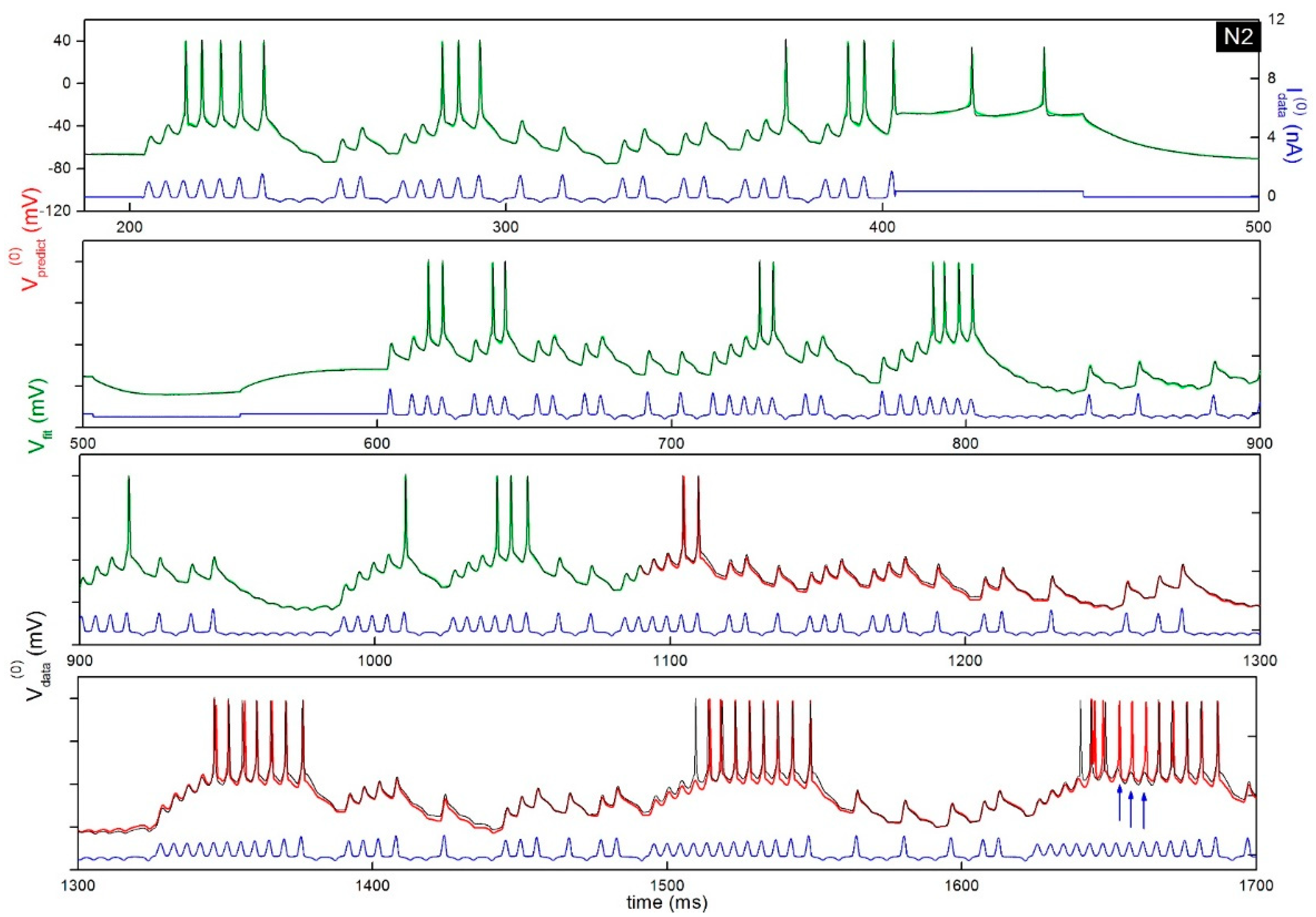
Biological considerations regarding the preferences of some ion channels to lie in greater density in the soma or the dendrites may also help select the ionic currents to include in the model. It is known, for example, that the density of calcium channels is greater in dendritic trees than in the soma [47,48,49,50], and hence, calcium channels may be omitted when modelling the soma compartment. In addition, single compartment models are often sufficient to give excellent predictions of neuronal activity [7,8,13,32,51]. The minute contribution of dendritic compartments may therefore be treated as a perturbation alongside model error. Figure 1 shows the process of constructing a complete model from electrophysiological recordings of a songbird neuron [7,8]. The conductance model used in this example is given in the supplementary information. The optimal fit of the model (green line) to the data (black line) is obtained by assimilating these data over a 590 ms time window. Once estimated, the parameters are inserted in the model equations. The completed model is then forward integrated from t = 1090 ms onwards (red trace), driven by the same current protocol applied to the interneuron (blue trace) [8]. Biological considerations also guide the choice of the parameter search intervals, which must be specified prior to assimilating the data.
2.2. Observability
Observability is a measure of how well the state and parameters of a conductance model can be inferred from measurements of the membrane voltage and other experimental observations. Takens’ theorem prescribes that all information needed to constrain the model is contained in an observation window of finite duration [52]. Aeyels [53] refined this argument by predicting that the number of observations be no less than 2L + 1, where L is the number of state variables in the system.
Electrophysiology and calcium imaging only allow a few state variables to be observed, namely the membrane voltage and calcium concentration. Gate variables mi and hi need to be inferred indirectly from time delayed observations of the membrane voltage. Parlitz et al. [54,55,56,57,58] and Letellier et al. [59,60,61] have studied the properties of the Jacobian matrix, embedding the state vector at time t in the time delayed measurements of the membrane voltage. They show that, when the embedding space is small, this matrix is singular in localized regions of dynamic maps. In those regions, the data do not contain enough information to uniquely constrain the neuron state, and hence, the system is not observable. Increasing the size of the embedding vector to match the number of state variables plus parameters was found to eliminate domains where the Jacobian is singular. The length of the assimilation window used to construct neuron models typically has 10,000–100,000 data points for models with less than 100 state variables and parameters [7,8,62,63,64]. This suggests that the volume of data is sufficient to fulfill the observability criterion. This has been empirically verified by reliably retrieving the parameters of the original model in twin experiments, where the assimilated data were generated by the same model, configured with known parameters. Twin experiments are the ultimate validation tool of well-posed inference problems where the model generating the data is fully known.
Naturally, increasing the number of state variables that can be matched to observation increases observability across the entire phase space [54,55], and also stabilizes convergence towards the global minimum of the objective functions, by reducing the occurrence of positive conditional Lyapunov exponents [65].
2.3. Identifiability
A model is identifiable if any two different sets of parameters produce different state trajectories starting from the same initial state [66,67]. Over-specified models may still be identifiable if unexpressed ion channels are filtered out (i.e., ), with all other ion channel parameters being fully constrained. This aside, over-specified models are not identifiable.
Identifiability is critically dependent on the stimulation protocol applied to the neuron. Unfortunately, parameter estimation has mainly focused on autonomous oscillators. Examples of parameter estimation from systems driven by an external force are comparatively few. Consequently, there is a need for further research on stimulation protocols that maximize identifiability. Central pattern generators are one example of autonomous oscillators where disparate parameters may yield the same oscillation patterns under no or tonic stimulation [34]. Similarly, no or tonic stimulation would fail to reveal adaptation in the electrical activity of a cell [68] from which calcium properties could not be identified. On the other hand, perturbing a central pattern generator, even with a modest variation in temperature or pH, is sufficient to switch between oscillatory modes [69,70,71] and in the process lift parameter degeneracy [40,41]. Maximum perturbation has been applied to neurons by designing current protocols that reveal adaptation mechanisms [7,8,14,32]. The design of such protocols has so far been guided by intuitive considerations based on the need to excite the hyperpolarized, sub-threshold, and depolarized regimes of the neuron, and to elicit the different response times of the neuron/circuit [7,8,14].
Identifiability may be achieved through careful design of current protocols. The aim is to retrieve the maximum of information from the data. The information contained in the current protocol may be quantified by the conditional Shannon entropy [72] relative to the conductance model. An alternative approach to testing identifiability has been suggested by Herman et al. [73] and Villaverde et al. [74]. Their method computes the Lie matrix linking the time derivatives of the data at different orders to the parameter vector at time t. Identifiability is validated by the matrix having full rank. If the matrix is singular, identifiability may be recovered by removing the matrix column(s) responsible for the singularity. This approach implies reparametrizing the model to remove functional overlap between parameters. Because models are meant to describe physical reality rather than the other way round, such simplifications rarely help characterize the underlying biology. Instead, Lie matrices are useful to validate the stimulation protocols that warrant the identifiability of neuron-based conductance models.
Numerical experiments have shown that identifiability criteria are fulfilled when current protocols elicit the full range of membrane voltage amplitudes and dynamics. Protocols that meet these conditions were found to constrain all model parameters to within 0.1% of their true value, independently of the waveform chosen for the current protocol.
2.4. Noise and Effect of Assimilation Window over Parameter Distribution Adaptive Sampling
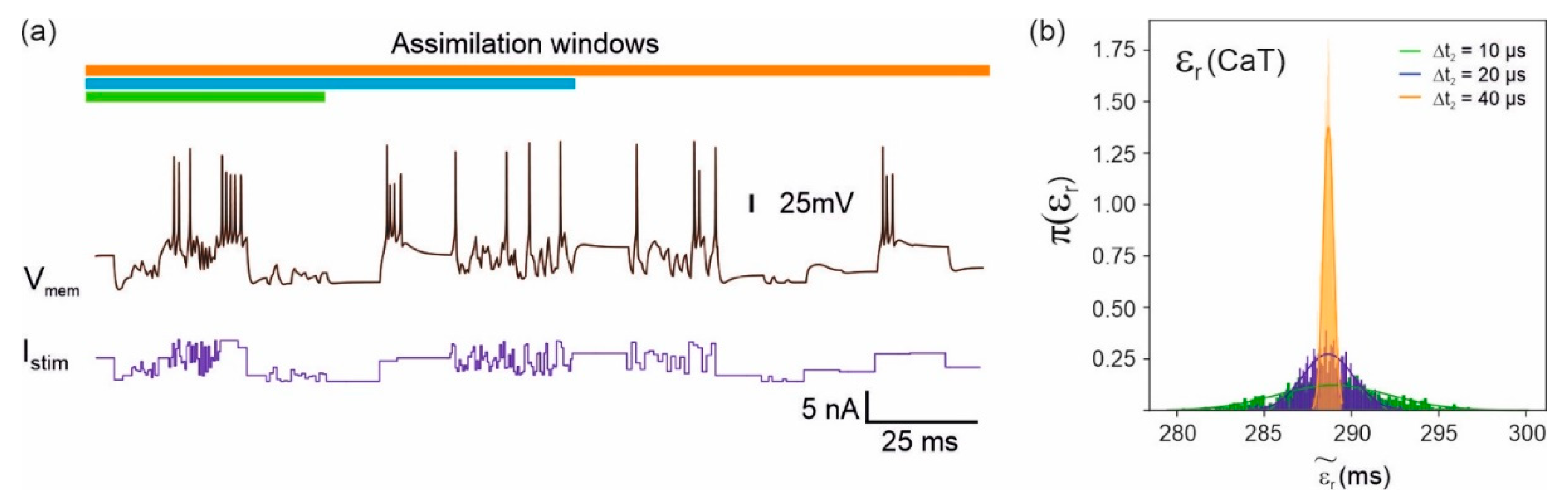
Noise in the membrane voltage introduces uncertainty in the parameter field. This is observed in the broadening of the posterior distribution function of extracted parameters (Figure 2), which is generally non-Gaussian [11]. Gaussian noise added to the current protocol has a comparatively small effect on parameter estimates, as it is integrated by the conductance model.
Measurement noise or intrinsic noise [75] may be smoothed {7,8] to improve parameter accuracy. Parameter accuracy may also be enhanced by increasing the duration of the assimilation window. In Figure 2, the effect of increasing the assimilation window is to narrow the posterior distribution function [11,76]. The assimilation window can be widened without increasing the size of the problem, using an adaptive mesh size. This works by selectively sampling action potentials at a faster rate than subthreshold oscillations across the assimilation window [11].
2.5. Stochastic Regularization of Convergence to Local Minima Vicinal to the Global Minimum
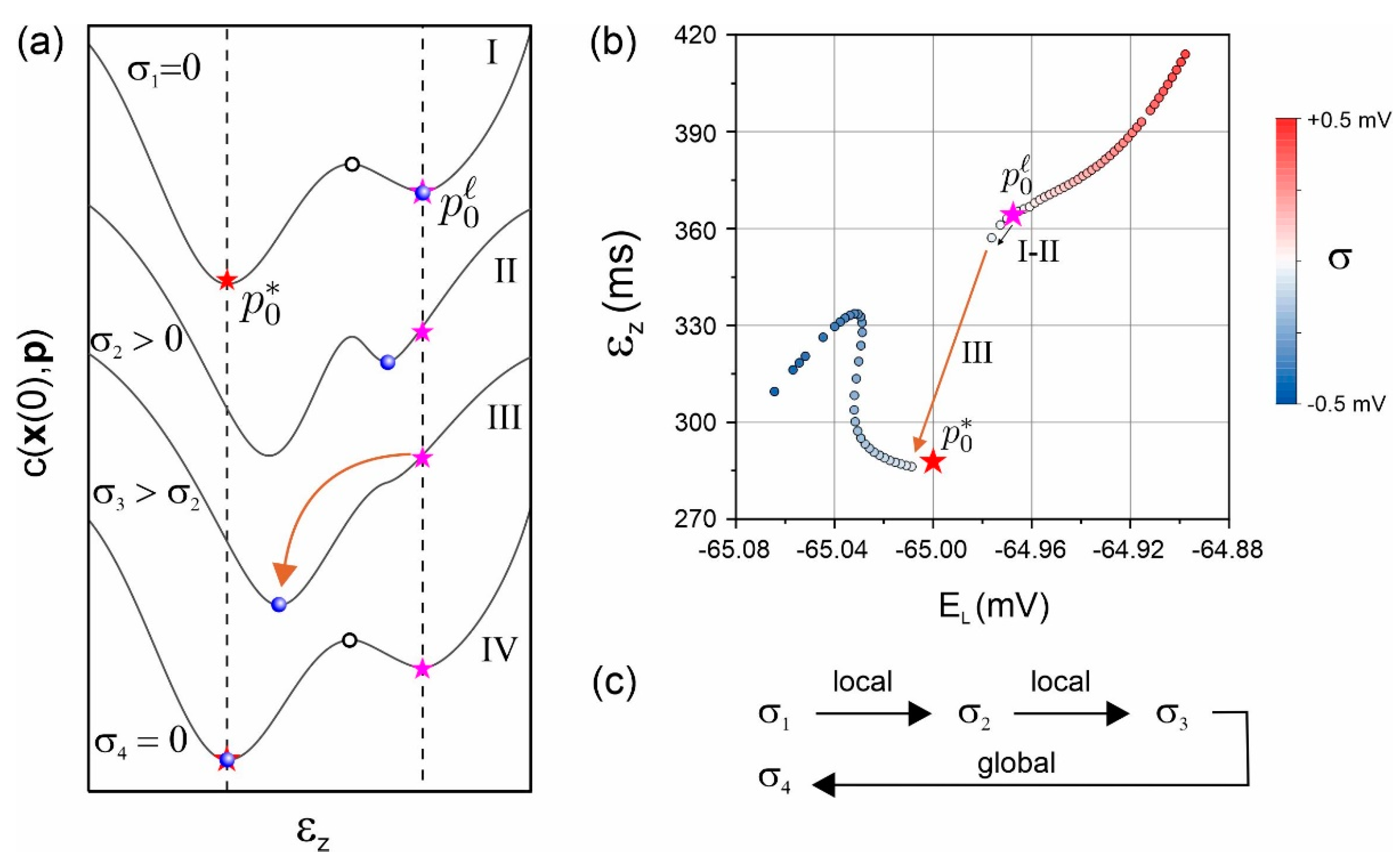
Erroneous parameter solutions may be obtained when the parameter search ends at a local minimum of the cost function. This is a rare occurrence which is usually observed when a vicinal local minimum has nearly the same data misfit error as the global minimum, and the difference between the two is smaller than the termination error of the algorithm. In this case, the true solution at the global minimum can still be obtained through the noise regularization method [11].
Noise has the effect of shifting the positions of local and global minima relative to one another in parameter space, as well as shifting these minima up in energy. An example is stochastic gradient descent [77,78]. The direction and magnitude of the shift depends both on the realization and the standard deviation of noise. By varying these noise parameters in a suitable manner, one can perturb the environment of the minima of the cost function and merge the local minimum, where the parameter search is arrived at, with the global minimum. The judicious management of additive noise until a merger has occurred, and subsequent removal of noise while tracking the return of the global minimum to the zero-noise level, can increase the accuracy on parameters beyond the limitations of gradient descent methods (Figure 3) [11].
3. Biological Neurons: Estimating Parameters from Guessed Models
The lack of knowledge on the exact biological model presents the principal challenge to the aim of characterizing ion channels. When the cost function only measures the fitting error between the time series data and one or more state variables, the optimum fit cannot represent the optimum parameters which we are seeking. Instead, some parameters will hit the boundaries of their search intervals in an attempt to compensate for model error. A model error term must therefore be added to the cost function to eliminate this compensation. The weight of the model error term must be carefully balanced with the data error term. This is done via their respective covariance matrices as we shall see below. If the model error is omitted from the cost function, parameter solutions will hit search interval boundaries to compensate for model error. Conversely, if the model error term carries a disproportionate weight, parameter solutions will be loosely constrained. This section discusses strategies which have been implemented, with various degrees of success, to obtain biological parameters from models whose error is known to be small. Models with residual error are defined here as models that (i) predict neuronal dynamics to a very high degree of accuracy under any current stimulation, and (ii) assign biologically realistic values to the thresholds and recovery times associated with the largest ionic conductances.
3.1. Including Model Error in the Cost Function
Model error is accounted for by adding a quadratic term in the cost function. This term avoids the strict enforcement of constraints when the model is guessed and necessarily departs from the true but unknown equations of motion :
The constraint is linearized at each mesh point of the assimilation window for each state variable giving constraints . The function will depend on the interpolation method used, for example: The cost function has a model error term that measures the discrepancies between the and across the assimilation window () and state variables (). To this, one adds the data error term that measures the distance between the membrane voltage in the experimental recording and the corresponding state variable in the model for :
This cost function is similar to the one used to infer the initial state of the atmosphere in meteorology [3]. It may also be formally derived from the action in Lagrangian mechanics [6]. A quadratic regularization term may added and treated as an additional state variable to remove the occurrence of positive Lyapunov exponents during convergence [79,80]. The are the diagonal elements of the covariance matrix of the model error. They establish a tradeoff between ignoring model error () and giving a greater weight to model error than data error, with the consequence that the model may fail to synchronize to the data (). The computation of these covariance matrices is an active area of research in data assimilation, which places emphasis on calculating majoration bounds of diagonal matrix elements [4]. This approach has been met with partial success in balancing data and model error in such a way that constraints (Equation (2)) are not enforced too strictly and do not send the model error term to zero in the cost function (Equation (3)). Note that in Equation (3), the covariance matrix of observation error is taken to be a unitary matrix. This is because consecutive measurements of the membrane voltage (or calcium concentration) are taken by the same apparatus which carries the same experimental error, hence, giving the same matrix elements on the diagonal. Measurements are also uncorrelated with one another, giving zero off-diagonal terms in the data error covariance matrix.
A simplification to computing the model error covariance matrix was proposed by Ye et al. [6,65]. They applied a majoration to the model error covariance matrix by retaining the error on a single state variable preferably the one that is the most sensitive to model error. The model error on was weighted by a single adjustable hyperparameter which was varied to optimally balance data and model error. This parameter expresses the degree of confidence one has in the model: the smaller the value of R, the lower the confidence in the model constraint:
Although Ye et al. [65] did not directly assimilate erroneous models, they studied the convergence of data assimilation as a function of as the number of state variables accessible to observation was incremented. They obtained an optimum value of where the sum of the data and model error passes through a minimum. Current research efforts are directed to engineering the covariance matrices of model error to obtain stable parameter estimates when model error is gradually switched on.
3.2. Supplementing Gradient Descent with Statistical Inference
Current clamp recordings of the membrane voltage, , may be written as the sum of the useful signal, , and a small error component, accounting for noise and model error. The cost function:
defines the energy surface whose minimum we seek. This total energy may be decomposed as the sum of a free energy, , and a random energy, as [8]:
where
and
Minimizing the cost function by a deterministic process such as gradient descent only minimizes the free energy part. The misfit error can only be minimized by statistical inference. Since we have assumed small experimental error, the misfit error determines the surface of an ellipsoid centered on the optimal parameter solution . This ellipsoid is given by the second order term in the Taylor expansion of the cost function, where is the Hessian at the site of .
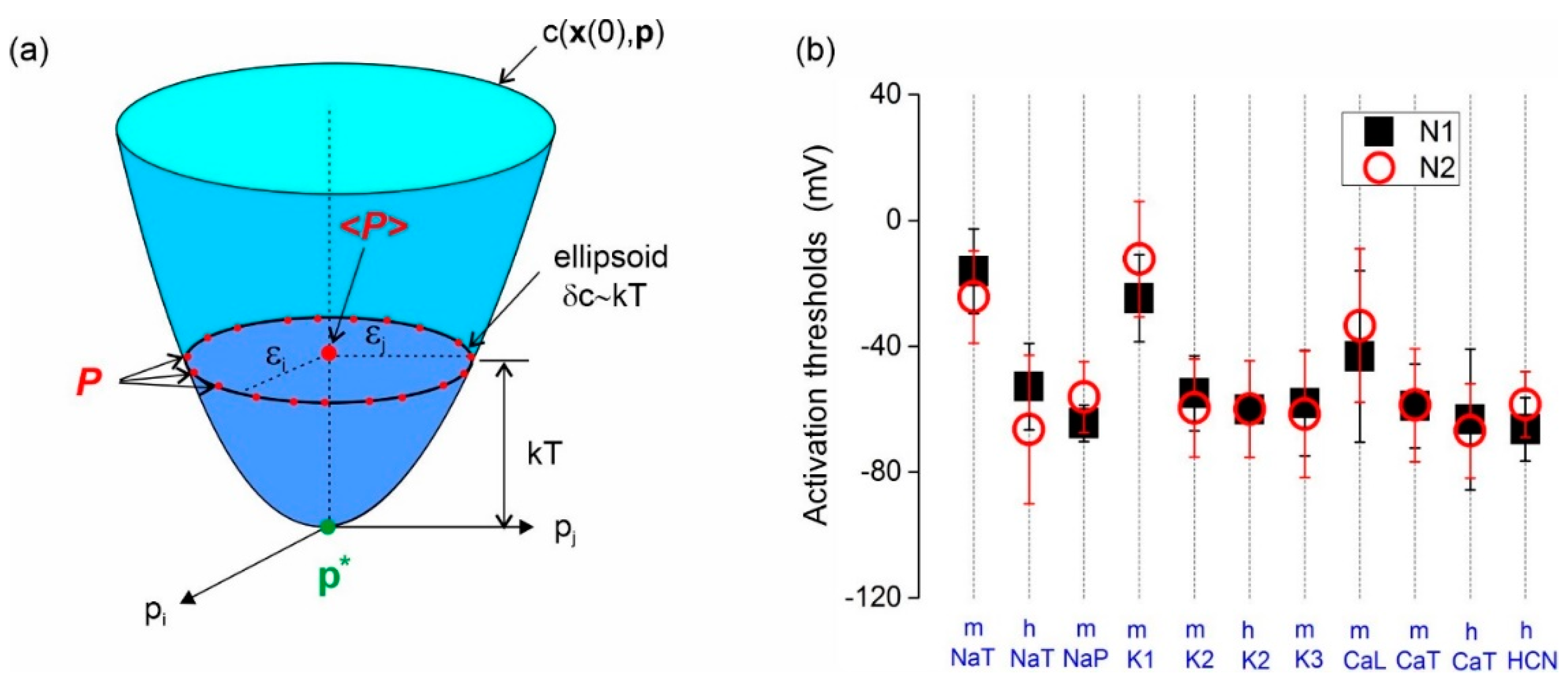
Starting the search of parameters from different initial guesses will generate parameter solutions, , distributed across this ellipsoid surface (Figure 4a). The true solution may therefore be approached by taking the mean value of the statistical sample of solutions derived from K initial guesses.
The approach has been successful in estimating the parameters of interneurons from the songbird high vocal center [8]. Figure 4b shows the activation and inactivation thresholds obtained by averaging the parameter solutions emanating from 84 initial guesses. These are the gate thresholds of all ion channels expressed in two interneurons, N1 and N2. The variance (vertical bars) indicates the dispersion of the underlying values. The average thresholds (dots/square symbols) otherwise become remarkably consistent across the two interneurons [8]. This consistency strongly suggests that averaging the thresholds obtained by gradient descent gives sensible estimates of the true biological thresholds. Similar consistency was obtained across ionic conductances and recovery time constants. The variance of the latter was, however, greater.
3.3. Aggregate State Variables
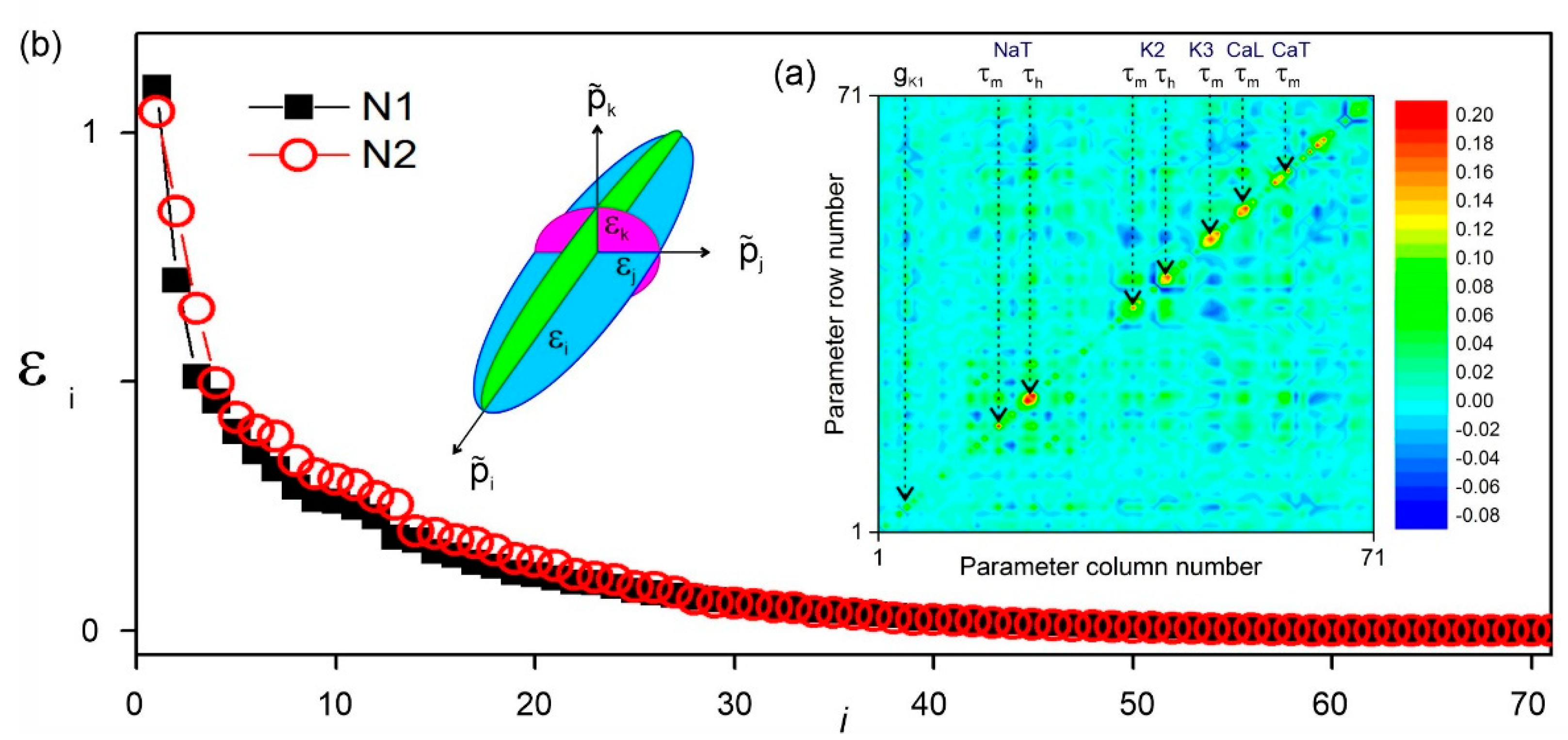
One effect of model error is to transform the minima of the cost function into deep valleys that correlate two or more parameters. The data misfit ellipsoid (Figure 4a) subsequently becomes spiky. This can be seen in the spectrum of the principal axes calculated from the inverse covariance matrix of the parameters from a songbird neuron [8]. This spectrum, shown in Figure 5, has an exponential distribution with a few outliers at . Examination of the covariance matrix of the estimated parameters (inset) identifies the recovery time constants of the ion channels as the most loosely constrained of all the parameters. This is not surprising as they enter the argument of exponentials describing the kinetics of the gate variables. The covariance matrix also suggests that parameter correlations are greater within the subset of parameters of each ion channel.
A strategy to extract biological information is to evaluate compound quantities that integrate correlations between more fundamental parameters. Ionic currents, or the amount of ionic charge transferred per action potential, may be reconstructed from parameter estimates of maximal ionic conductances, gate recovery times, and voltage thresholds. The reconstructed quantities often carry a much lower uncertainty than the estimates of model parameters. Morris et al. [81] have recently used this approach to predict the amount of charge transfer through individual ion channels modulated by inhibitor drugs. Data assimilation was able to predict the selectivity and potency of inhibitor drugs in good agreement with IC50 analysis, by estimating the amount of charge transferred across each ion channel before and after inhibition.
4. Discussion
Gradient descent algorithms have reliably recovered the 10–100 parameters of neuron-based conductance models. When the problem is well-posed, these parameters are systematically found to lie within 0.1% of the true parameter values. These are the parameters set in the model used to synthesize the time series data. An accuracy better than 0.1% supposes that the criteria of observability and identifiability are satisfied. Observability can be further improved by increasing the number of state variables which are observed. This means complementing electrophysiological recordings with calcium [82] or optogenetic recordings [83]. More observed state variables also means that the parameter search becomes less likely to develop positive Lyapunov exponents [65,82,84,85] and to converge [54,55]. Identifiability is conditional to the nature of stimulation applied to the system. Although much theoretical work remains to be done to design stimulation protocols that transfer a maximum of information from the data to the model, numerical studies show that protocols eliciting both hyperpolarized and depolarized oscillations, while covering the full spectrum of ionic gate kinetics, are sufficient to recover all original parameters in twin experiments. Noise in experimental data is easily dealt with by smoothing membrane voltage time series to reduce the uncertainty on parameters. Additive Gaussian noise may be used in a constructive manner to regularize convergence towards the global minimum of the cost function.
Currently the major roadblock in estimating the parameters of neurons is model error. Conventional approaches insert error in the cost function alongside data error. This requires balancing data and model error, either through ab-initio calculations of the model error covariance matrix, or by using a variational parameter such as as a majoration of model error. In either case, the data assimilation algorithm must relax the enforcement of constraints without sending the model error term of the cost function to zero. Reservoir computing [1] can, in principle, also help correct model error. The non-physical models, built by training a neural network on time series data, can be used to identify error in the conductance equations. The excellent predictions of neuron oscillations made by conductance models have suggested two empirical methods which revealed ion channel properties in good agreement with voltage clamp measurements and IC50 analysis. The first approach consists of taking the mean expectation value of a statistical sample of parameters computed from many different initial guesses. This method was shown to give consistent activation thresholds and ion channel conductances across the complement of ion channels of nominally equivalent songbird neurons. The second approach used the observation that parameter correlations tend to be greatest within each ion channel. We showed that quantities reconstructed from these parameter subsets—the charge transferred per action potential and the ionic current—could be predicted with enough accuracy to identify which ion channels were inhibited when an inhibitor drug was applied and the potency of the drug. Data assimilation has also successfully optimized conductance models derived from the IV characteristics of neuromorphic circuits [51,86]. The conditioning of neuromorphic circuits [69,71] with the parameters that produce the correct adaptation to stimuli is generating considerable interest for bioelectronic medicine [87] and brain–machine interfaces [88,89].
Supplementary Materials
The following supporting information can be downloaded at: https://0-www-mdpi-com.brum.beds.ac.uk/article/10.3390/a15050168/s1, Figure S1: The generic rate equation of a gate variable, here . is the threshold of the sigmoidal activation. is the width of the transition from the open to the closed state of the gate. gives an activation curve; inactivation. The recovery time of most gate variables has a Bell-shaped curve defined by 3 parameters: . This dependence describes all activation gates and almost all inactivation gates the exception being the K2 and CaT inactivation recovery times which exhibit a rectifying behaviour and a biexponential dependence respectively; Figure S2: Mathematical form of the 9 ionic currents used to model the songbird neuron in Figure 1 of the manuscript.
Funding
This research was funded by the European Union’s Horizon 2020 Future Emerging Technologies Program under grant No. 732170.
Institutional Review Board Statement
Not applicable.
Informed Consent Statement
Not applicable.
Data Availability Statement
Not applicable.
Acknowledgments
This work has benefitted from many discussions with colleagues: Henry Abarbanel (San Diego), Paul Morris (Cambridge), Timothy O’Reilly (Cambridge), Joseph Taylor (Bath), and Stephen Wells (Bath).
Conflicts of Interest
The author declares no conflict of interest. The funders had no role in the design of the study; in the collection, analyses, or interpretation of data; in the writing of the manuscript, or in the decision to publish the results.
References
- Pathak, J.; Hunt, B.; Girvan, M.; Lu, Z.; Ott, E. Model-Free Prediction of Large Spatiotemporally Chaotic Systems from Data: A Reservoir Computing Approach. Phys. Rev. Lett. 2018, 120, 024102. [Google Scholar] [CrossRef] [PubMed] [Green Version]
- Silver, D.; Schrittwieser, J.; Simonyan, K.; Antonoglou, I.; Huang, A.; Guez, A.; Hubert, T.; Baker, L.; Lai, M.; Bolton, A.; et al. Mastering the game of Go without human knowledge. Nature 2017, 550, 354–359. [Google Scholar] [CrossRef] [PubMed]
- Kalnay, E. Atmospheric Modeling, Data Assimilation and Predictability; Cambridge University Press: Cambridge, UK, 2003. [Google Scholar]
- Tabeart, J.M.; Dance, S.L.; Haben, S.A.; Lawless, A.S.; Nichols, N.K.; Waller, J.A. The conditioning of least-squares problems in variational data assimilation. Numer. Linear Algebra Appl. 2018, 25, e2165. [Google Scholar] [CrossRef]
- Abarbanel, H.D.I. Predicting the Future: Completing Models of Observed Complex Systems; Springer: Heidelberg, Germany, 2013. [Google Scholar]
- Abarbanel, H.D.I. The Statistical Physics of Data Assimilation and Machine Learning; Cambridge University Press: Cambridge, UK, 2022. [Google Scholar] [CrossRef]
- Meliza, C.D.; Kostuk, M.; Huang, H.; Nogaret, A.; Margoliash, D.; Abarbanel, H.D.I. Estimating parameters and predicting membrane voltages with conductance-based neuron models. Biol. Cybern. 2014, 108, 495–516. [Google Scholar] [CrossRef]
- Nogaret, A.; Meliza, C.D.; Margoliash, D.; Abarbanel, H.D.I. Automatic Construction of Predictive Neuron Models through Large Scale Assimilation of Electrophysiological Data. Sci. Rep. 2016, 6, 32749. [Google Scholar] [CrossRef] [Green Version]
- Kostuk, M.; Toth, B.A.; Meliza, C.D.; Margoliash, D.; Abarbanel, H.D.I. Dynamical estimation of neuron and network properties II: Path integral Monte Carlo methods. Biol. Cybern. 2012, 106, 155–167. [Google Scholar] [CrossRef]
- Toth, B.A.; Kostuk, M.; Meliza, C.D.; Margoliash, D.; Abarbanel, H.D.I. Dynamical estimation of neuron and network properties I: Variational methods. Biol. Cybern. 2011, 105, 217–237. [Google Scholar] [CrossRef]
- Taylor, J.D.; Winnall, S.; Nogaret, A. Estimation of neuron parameters from imperfect observations. PLOS Comput. Biol. 2020, 16, e1008053. [Google Scholar] [CrossRef]
- Hartoyo, A.; Casdusch, P.J.; Lilley, D.T.J.; Hicks, D.J. Parameter estimation and identifiability in a neural population model for electro-cortical activity. PLoS Comp. Biol. 2019, 15, e1006694. [Google Scholar] [CrossRef] [Green Version]
- Brookings, T.; Goeritz, M.L.; Marder, E. Automatic parameter estimation of multicompartmental neuron models via minimization of trace error with control adjustment. J. Neurophysiol. 2014, 112, 2332–2348. [Google Scholar] [CrossRef] [Green Version]
- Armstrong, E. Statistical data assimilation for estimating electrophysiology simultaneously with connectivity within a biological neuronal network. Phys. Rev. E 2020, 101, 012415. [Google Scholar] [CrossRef] [PubMed] [Green Version]
- Armstrong, E.; Abarbanel, H.D.I. Model of the songbird nucleus HVC as a network of central pattern generators. J. Neurophysiol. 2016, 116, 2405–2419. [Google Scholar] [CrossRef] [PubMed] [Green Version]
- Prinz, A.A.; Billimoria, C.P.; Marder, E. Alternative to hand-tuning conductance-based models: Constriction and analysis of databases of model neurons. J. Neurophysiol. 2003, 90, 4015. [Google Scholar] [CrossRef] [PubMed]
- Gouwens, N.W.; Sorensen, S.A.; Baftizadeh, F.; Budzillo, A.; Lee, B.R.; Jarsky, T.; Alfiler, L.; Baker, K.; Barkan, E.; Berry, K.; et al. Integrated Morphoelectric and Transcriptomic Classification of Cortical GABAergic Cells. Cell 2020, 183, 953.e19. [Google Scholar] [CrossRef] [PubMed]
- Griffin, M.; Khan, R.; Basu, S.; Smith, S. Ion Channels as Therapeutic Targets in High Grade Gliomas. Cancers 2020, 12, 3068. [Google Scholar] [CrossRef] [PubMed]
- Molenaar, R.J. Ion Channels in Glioblastoma. ISRN Neurol. 2011, 2011, 590249. [Google Scholar] [CrossRef] [Green Version]
- Chakroborty, S.; Stutzmann, G.E. Calcium channelopathies and Alzheimer’s disease: Insight into therapeutic success and failures. Eur. J. Pharmacol. 2014, 739, 83–95. [Google Scholar] [CrossRef]
- Huys, Q.J.M.; Ahrens, M.B.; Paninski, L. Efficient Estimation of Detailed Single-Neuron Models. J. Neurophysiol. 2006, 96, 872–890. [Google Scholar] [CrossRef]
- Eiben, A.E.; Smith, J.E. Introduction to Evolutionary Computing; Springer: Heidelberg, Germany, 2003. [Google Scholar]
- Druckmann, S.; Banitt, Y.; A Gidon, A.; Schürmann, F.; Markram, H.; Segev, I. A novel multiple objective optimization framework for constraining conductance-based neuron models by experimental data. Front. Neurosci. 2007, 1, 7–18. [Google Scholar] [CrossRef] [Green Version]
- Kobayashi, R.; Tsubo, Y.; Shinomoto, S. Made-to-order spiking neuron model equipped with a multi-timescale adaptive threshold. Front. Comput. Neurosci. 2009, 3, 9. [Google Scholar] [CrossRef] [Green Version]
- Marasco, A.; Limongiello, A.; Migliore, M. Fast and accurate low-dimensional reduction of biophysically detailed neuron models. Sci. Rep. 2012, 2, srep00928. [Google Scholar] [CrossRef] [PubMed]
- Achard, P.; De Schutter, E. Complex Parameter Landscape for a Complex Neuron Model. PLoS Comput. Biol. 2006, 2, e94. [Google Scholar] [CrossRef] [PubMed] [Green Version]
- Buhry, L.; Pace, M.; Saïghi, S. Global parameter estimation of an Hodgkin–Huxley formalism using membrane voltage recordings: Application to neuro-mimetic analog integrated circuits. Neurocomputing 2012, 81, 75–85. [Google Scholar] [CrossRef]
- Hendrickson, E.B.; Edgerton, J.R.; Jaeger, D. The use of automated parameter searches to improve ion channel kinetics for neural modeling. J. Comput. Neurosci. 2011, 31, 329–346. [Google Scholar] [CrossRef] [PubMed]
- Kennedy, J.; Eberhardt, R. Particle swarm optimization. In Proceedings of the ICNN’95-International Conference On Neural Networks IEEE, Perth, Australia, 27 November–1 December 1995; pp. 1942–1948. [Google Scholar]
- Wächter, A.; Biegler, L.T. On the implementation of an interior-point filter line-search algorithm for large-scale nonlinear programming. Math. Program. 2005, 106, 25–57. [Google Scholar] [CrossRef]
- Boyd, S.; Vanderberghe, L. Convex Optimization; Cambridge University Press: Cambridge, UK, 2004. [Google Scholar]
- Vavoulis, D.V.; Straub, V.; Aston, J.A.D.; Feng, J. A Self-Organizing State-Space-Model Approach for Parameter Estimation in Hodgkin-Huxley-Type Models of Single Neurons. PLoS Comput. Biol. 2012, 8, e1002401. [Google Scholar] [CrossRef]
- Marder, E.; Taylor, A.L. Multiple models to capture the variability in biological neurons and networks. Nat. Neurosci. 2011, 14, 133–138. [Google Scholar] [CrossRef]
- A Prinz, A.; Bucher, D.; Marder, E. Similar network activity from disparate circuit parameters. Nat. Neurosci. 2004, 7, 1345–1352. [Google Scholar] [CrossRef]
- Goaillard, J.-M.; Taylor, A.L.; Schulz, D.; Marder, E. Functional consequences of animal-to-animal variation in circuit parameters. Nat. Neurosci. 2009, 12, 1424–1430. [Google Scholar] [CrossRef] [Green Version]
- Marder, E.; Goaillard, J.-M. Variability, compensation and homeostasis in neuron and network function. Nat. Rev. Neurosci. 2006, 7, 563–574. [Google Scholar] [CrossRef]
- Lederman, D.; Patel, R.; Itani, O.; Rotstein, H.G. Parameter Estimation in the Age of Degeneracy and Unidentifiability. Mathematics 2022, 10, 170. [Google Scholar] [CrossRef]
- O’Leary, T.; Sutton, A.C.; Marder, E. Computational models in the age of large data sets. Curr. Opin. Neurobiol. 2015, 32, 87. [Google Scholar] [CrossRef] [PubMed] [Green Version]
- Gutenkunst, R.N.; Waterfall, J.; Casey, F.P.; Brown, K.S.; Myers, C.R.; Sethna, J.P. Universally Sloppy Parameter Sensitivities in Systems Biology Models. PLOS Comput. Biol. 2007, 3, 1871–1878. [Google Scholar] [CrossRef] [PubMed] [Green Version]
- Kushinsky, D.; Morozova, E.O.; Marder, E. In vivo effects of temperature on the heart and pyloric rhythms in the crab, Cancer borealis. J. Exp. Biol. 2019, 222, jeb199190. [Google Scholar] [CrossRef] [Green Version]
- Haley, J.A.; Hampton, D.; Marder, E. Two central pattern generators from the crab, Cancer borealis respond robustly and differentially to extreme extracellular pH. eLife 2018, 7, e41977. [Google Scholar] [CrossRef]
- Hodgkin, A.L.; Huxley, A.F. A quantitative description of membrane current and its application to conduction and excitation in nerve. J. Physiol. 1952, 117, 500–544. [Google Scholar] [CrossRef]
- Huguenard, J.R.; Mc Cormick, D.A. Simulation of the currents involved in rhythmic oscillations in thalamic neurons. J. Neurophysiol. 1992, 68, 1373. [Google Scholar] [CrossRef]
- Otopalik, A.G.; Sutton, A.C.; Banghart, M.; Marder, E. When complex neuronal structures may not matter. eLife 2017, 6, 2066. [Google Scholar] [CrossRef] [Green Version]
- Lilacci, G.; Khammash, M. Parameter estimation and model selection in computational biology. PLoS Comp. Biol. 2012, 6, e1000696. [Google Scholar] [CrossRef] [Green Version]
- Kahl, D.; Kschischo, M. Searching for Errors in Models of Complex Dynamic Systems. Front. Physiol. 2021, 11, 612590. [Google Scholar] [CrossRef]
- Markram, H.; Sakman, B. Calcium transients in dendrites of neocortical neurons evoked by single threshold excitatory postsynaptic potentials via low-voltage-activated calcium channels. Proc. Nat. Acad. Sci. USA 1994, 91, 5207. [Google Scholar] [CrossRef] [PubMed] [Green Version]
- Del Negro, C.A.; Morgado-Valle, C.; Hayes, J.A.; Mackay, D.D.; Pace, R.W.; Crowder, E.A.; Feldman, J.L. Sodium and Calcium Current-Mediated Pacemaker Neurons and Respiratory Rhythm Generation. J. Neurosci. 2005, 25, 446–453. [Google Scholar] [CrossRef] [PubMed] [Green Version]
- Kastellakis, G.; Silva, A.J.; Poirazi, P. Linking Memories across Time via Neuronal and Dendritic Overlaps in Model Neurons with Active Dendrites. Cell Rep. 2016, 17, 1491–1504. [Google Scholar] [CrossRef] [PubMed] [Green Version]
- Spruston, N.; Schiller, Y.; Stuart, G.; Sakmann, B. Activity-Dependent Action Potential Invasion and Calcium Influx into Hippocampal CA1 Dendrites. Science 1995, 268, 297–300. [Google Scholar] [CrossRef]
- Abu-Hassan, K.; Taylor, J.D.; Morris, P.G.; Donati, E.; Bortolotto, Z.A.; Indiveri, G.; Paton, J.F.R.; Nogaret, A. Optimal neuron models. Nat. Commun. 2019, 10, 5309. [Google Scholar] [CrossRef]
- Takens, F. Detecting Strange Attractors in Turbulence in Dynamic Systems in Turbulence; Springer: Warwick, UK, 1981; pp. 366–381. [Google Scholar]
- Aeyels, D. Generic Observability of Differentiable Systems. SIAM J. Control Optim. 1981, 19, 595–603. [Google Scholar] [CrossRef]
- Parlitz, U.; Schumann-Bischoff, J.; Luther, S. Local observability of state variables and parameters in nonlinear modeling quantified by delay reconstruction. Chaos Interdiscip. J. Nonlinear Sci. 2014, 24, 24411. [Google Scholar] [CrossRef] [Green Version]
- Parlitz, U.; Schumann-Bischoff, J.; Luther, S. Quantifying uncertainty in state and parameter estimation. Phys. Rev. E 2014, 89, 050902. [Google Scholar] [CrossRef] [Green Version]
- Parlitz, U.; Merkwirth, C. Prediction of Spatiotemporal Time Series Based on Reconstructed Local States. Phys. Rev. Lett. 2000, 84, 1890–1893. [Google Scholar] [CrossRef]
- Schumann-Bischoff, J.; Parlitz, U. State and parameter estimation using unconstrained optimization. Phys. Rev. E 2011, 84, 056214. [Google Scholar] [CrossRef]
- Schumann-Bischoff, J.; Luther, S.; Parlitz, U. Estimability and dependency analysis of model parameters based on delay coordinates. Phys. Rev. E 2016, 94, 032221. [Google Scholar] [CrossRef] [PubMed]
- Letellier, C.; Aguirre, L.; Maquet, J. How the choice of the observable may influence the analysis of nonlinear dynamical systems. Commun. Nonlinear Sci. Numer. Simul. 2006, 11, 555–576. [Google Scholar] [CrossRef]
- Letellier, C.; Aguirre, L.A.; Maquet, J. Relation between observability and differential embeddings for nonlinear dynamics. Phys. Rev. E 2005, 71, 066213. [Google Scholar] [CrossRef] [PubMed] [Green Version]
- Aguirre, L.A.; Portes, L.L.; Letellier, C. Observability and synchronization of neuron models. Chaos Interdiscip. J. Nonlinear Sci. 2017, 27, 103103. [Google Scholar] [CrossRef] [Green Version]
- Tabak, J.; Moore, L. Simulation and parameter estimation study of a simple neuronal model of rhythm generation: Role of NMDA and non-NMDA receptors. J. Comput. Neurosci. 1998, 5, 209–235. [Google Scholar] [CrossRef]
- Moye, M.J.; Diekman, C.O. Data Assimilation Methods for Neuronal State and Parameter Estimation. J. Math. Neurosci. 2018, 8, 11. [Google Scholar] [CrossRef]
- Rey, D.; Eldridge, M.; Morone, U.; Abarbanel, H.D.I.; Parlitz, U.; Schumann-Bischoff, J. Using waveform information in nonlinear data assimilation. Phys. Rev. E 2014, 90, 062916. [Google Scholar] [CrossRef] [Green Version]
- Ye, J.; Rey, D.; Kadakia, N.; Eldridge, M.; Morone, U.I.; Rozdeba, P.; Abarbanel, H.D.I.; Quinn, J.C. Systematic variational method for statistical nonlinear state and parameter estimation. Phys. Rev. E 2015, 92, 052901. [Google Scholar] [CrossRef] [Green Version]
- Yu, W.; Chen, G.; Cao, J.; Lü, J.; Parlitz, U. Parameter identification of dynamical systems from time series. Phys. Rev. E 2007, 75, 067201. [Google Scholar] [CrossRef]
- Raue, A.; Becker, V.; Klingmüller, U.; Timmer, J. Identifiability and observability analysis for experimental design in nonlinear dynamical models. Chaos Interdiscip. J. Nonlinear Sci. 2010, 20, 045105. [Google Scholar] [CrossRef]
- Kuwana, S.-I.; Tsunekawa, N.; Yanagawa, Y.; Okada, Y.; Kuribayashi, J.; Obata, K. Electrophysiological and morphological characteristics of GABAergic respiratory neurons in the mouse pre-Bötzinger complex. Eur. J. Neurosci. 2006, 23, 667–674. [Google Scholar] [CrossRef] [PubMed]
- Chauhan, A.S.; Taylor, J.; Nogaret, A. Local inhibitory networks support up to (N−1)!/lnN2 limit cycles in the presence of electronic noise and heterogeneity. Phys. Rev. Res. 2021, 3, 043097. [Google Scholar] [CrossRef]
- Nogaret, A.; King, A. Inhibition delay increases neural network capacity through Sterling transform. Phys. Rev. E 2018, 97, 030301. [Google Scholar] [CrossRef] [PubMed] [Green Version]
- Chauhan, A.S.; Taylor, J.D.; Nogaret, A. Dual Mechanism for the Emergence of Synchronization in Inhibitory Neural Networks. Sci. Rep. 2018, 8, 11431. [Google Scholar] [CrossRef] [Green Version]
- Cover, T.M.; Thomas, J.A. Elements of Information Theory; Wiley: Hoboken, NJ, USA, 1991. [Google Scholar]
- Hermann, R.; Krener, A. Nonlinear controllability and observability. IEEE Trans. Autom. Control 1977, 22, 728–740. [Google Scholar] [CrossRef] [Green Version]
- Villaverde, A.F.; Barreiro, A.; Papachristodoulou, A. Structural Identifiability of Dynamic Systems Biology Models. PLOS Comput. Biol. 2016, 12, e1005153. [Google Scholar] [CrossRef] [Green Version]
- Faisal, A.A.; Selen, L.P.J.; Wolpert, D.M. Noise in the nervous system. Nat. Rev. Neurosci. 2006, 9, 292. [Google Scholar] [CrossRef]
- Blayo, E.; Bouquet, M.; Cosme, E.; Cugliandolo, L.F. Advanced Data Assimilation for Geosciences. Lecture Notes of the Les Houches School of Physics: Special Issue; Oxford University Press: Oxford, UK, 2012. [Google Scholar]
- Morse, G.; Stanley, K.O. Simple Evolutionary Optimization Can Rival Stochastic Gradient Descent in Neural Networks. Proc. GECCO 2016, 477–484. [Google Scholar] [CrossRef] [Green Version]
- Bottou, L.; Bousquet, O. The tradeoffs of large-scale learning. Adv. Neural Inf. Processing Syst. 2008, 20, 161. [Google Scholar]
- Abarbanel, H.D.I.; Creveling, D.R.; Jeanne, J.M. Estimation of parameters in nonlinear systems using balanced synchronization. Phys. Rev. E 2008, 77, 016208. [Google Scholar] [CrossRef] [Green Version]
- Abarbanel, H.D.I.; Kostuk, M.; Whartenby, W. Data assimilation with regularized nonlinear instabilities. Q. J. R. Meteorol. Soc. 2010, 136, 769–783. [Google Scholar] [CrossRef]
- Morris, P.G.; Taylor, J.D.; Wells, S.A.; Nogaret, A. Prediction of Pharmacologically-Induced Changes in Specific Ion Channels by Assimilation of Neuronal Membrane Voltage Data. UK Patent 2206436.4, 2022. [Google Scholar]
- Deneux, T.; Kaszas, A.; Szalay, G.; Katona, G.; Lakner, T.; Grinvald, A.; Rózsa, B.; Vanzetta, I. Accurate spike estimation from noisy calcium signals for ultra-fast three-dimensional imaging of large neuronal populations in-vivo. Nat. Commun. 2016, 7, 12190. [Google Scholar] [CrossRef] [PubMed]
- Davidović, A.; Chait, R.; Batt, G.; Ruess, J. Parameter inference for stochastic biochemical models from perturbation experiments parallelized at the single cell level. PLoS Comput. Biol. 2022, 18, e1009950. [Google Scholar] [CrossRef]
- Tikhonov, A.N. On the stability of inverse problems. Doklaady Akad. Nauk. SSSR 1943, 39, 195. [Google Scholar]
- Creveling, D.R.; Gill, P.E.; Abarbanel, H.D. State and parameter estimation in nonlinear systems as an optimal tracking problem. Phys. Lett. A 2008, 372, 2640–2644. [Google Scholar] [CrossRef]
- Wang, J.; Breen, D.; Akinin, A.; Broccard, F.D.; Abarbanel, H.D.I.; Cauwenberghs, G. Assimilation of Biophysical Neuronal Dynamics in Neuromorphic VLSI. IEEE Trans. Biomed. Circuits Syst. 2017, 11, 1258–1270. [Google Scholar] [CrossRef]
- O’Callaghan, E.L.; Chauhan, A.S.; Zhao, L.; Lataro, R.M.; Salgado, H.C.; Nogaret, A.; Paton, J.F.R. Utility of a novel biofeedback device for within breadth modulation of heart rate in rats: A quantitative comparison of vagus nerve vs right atrial pacing. Front. Physiol. 2016, 7, 27. [Google Scholar]
- Jiang, S.; Patel, D.C.; Kim, J.; Yang, S.; Mills, W.A.; Zhang, Y.; Wang, K.; Feng, Z.; Vijayan, S.; Cai, W.; et al. Spatially expandable fiber-based probes as a multifunctional deep brain interface. Nat. Commun. 2020, 11, 6115. [Google Scholar] [CrossRef]
- Trautmann, E.M.; O’Shea, D.J.; Sun, X.; Marshel, J.H.; Crow, A.; Hsueh, B.; Vesuna, S.; Cofer, L.; Bohner, G.; Allen, W.; et al. Dendritic calcium signals in rhesus macaque motor cortex drive an optical brain-computer interface. Nat. Commun. 2021, 12, 3689. [Google Scholar] [CrossRef]
Figure 1.
Construction of a model neuron from electrophysiological recordings of interneurons from the songbird brain. The model (green trace) is synchronized to the membrane voltage time series (black trace) of an interneuron of the songbird brain. The model trace is directly overlayed over the data. The neuron membrane voltage was recorded under current stimulation by a protocol (blue trace) mixing chaotic oscillations (Lorenz system) and long current steps. Parameters are obtained from the model that best synchronizes its membrane voltage state variable to the data (green trace). This optimal model is then used to forward integrate the current protocol and predict the future state of the neuron (red trace). Here, note that the predicted membrane voltage occasionally departs from the data (black line). The blue arrows show the position of three action potentials missing from the data. These are missing because the current protocol at around 1650 ms is exactly the same as the one giving the continuous bursts at 1350 ms and 1550 ms. The missing action potentials are likely due to input from other neurons in the slide, which cannot be completely eliminated through inhibitors.

Figure 2.
Effect of the length of the data assimilation window on parameter accuracy. (a) The model data (black line) were obtained by stimulating the model equations with the current protocol (blue line). A small amount of Gaussian noise was added to introduce uncertainty in the parameters inferred back from the data. Parameters were estimated from three assimilation windows of increasing duration but incorporating the same number of data points, thanks to an adaptive step size applied to subthreshold oscillations. (b) Posterior distribution functions of one model parameter (gate recovery time constant) corresponding to the three assimilation windows [11].

Figure 3.
Regularization by noise. (a) The cost function plotted as a function of one parameter has local minimum in the vicinity of the global minimum . The parameter estimation algorithm started from an initial guess at the local minimum (pink star). Then, the amplitude of noise was increased. Until a critical value, the parameter solution remains in the local minimum but shifts (blue dot). Above this critical value, at , the local minima and the global minimum merge, causing an abrupt jump of the solution into the (noise shifted) global minimum. The global solution above then need to be inserted as input to the parameter estimation algorithm, and then, noise is progressively decreased to zero to obtain the global minimum at zero noise. (b) Trajectory of the neuron parameter vector projected in two dimensions as noise is varied. A jump is observed from the local to the global solution. (c) Schematics of the noise annealing protocol [11].

Figure 4.
(a) Schematic of the cost function near the global minimum. The parameters () estimated from different parameter guesses distribute on the ellipsoid surface . This ellipsoid effectively broadens the global minimum proportionally to the error variance. Actual parameters are approached by averaging over all initial guesses, since . (b) Activation thresholds (m) and inactivation thresholds (h) obtained by averaging over 84 values of random vector . The average thresholds are shown for two interneurons, N1 and N2, of the songbird high vocal center. The ion channels are transient sodium (NaT), persistent sodium (NaP), potassium (K1), inactivating potassium (K3), muscarinic (K3), high threshold calcium (CaL), low threshold calcium (CaT), and hyperpolarization activated channel (HCN) [8].

Figure 5.
Correlations between estimated parameters. (a) Covariance matrix of the 71 parameters of a multichannel conductance models, synchronized to electrophysiological recordings of a songbird neuron. A total of 81 sets of parameters were estimated from different assimilation windows to generate the statistical sample used to compute the covariance. Parameters pertaining to each ion channel tend to be more correlated. The greater error/variance is in the recovery time constants of ionic gates (). The principal values of the covariance matrix give the length of the principal semi-axes of the data misfit ellipsoid . (b) Spectrum of principal values of the covariance matrix.

Publisher’s Note: MDPI stays neutral with regard to jurisdictional claims in published maps and institutional affiliations. |
© 2022 by the author. Licensee MDPI, Basel, Switzerland. This article is an open access article distributed under the terms and conditions of the Creative Commons Attribution (CC BY) license (https://creativecommons.org/licenses/by/4.0/).
Share and Cite
MDPI and ACS Style
Nogaret, A. Approaches to Parameter Estimation from Model Neurons and Biological Neurons. Algorithms 2022, 15, 168. https://0-doi-org.brum.beds.ac.uk/10.3390/a15050168
AMA Style
Nogaret A. Approaches to Parameter Estimation from Model Neurons and Biological Neurons. Algorithms. 2022; 15(5):168. https://0-doi-org.brum.beds.ac.uk/10.3390/a15050168
Chicago/Turabian StyleNogaret, Alain. 2022. "Approaches to Parameter Estimation from Model Neurons and Biological Neurons" Algorithms 15, no. 5: 168. https://0-doi-org.brum.beds.ac.uk/10.3390/a15050168
Note that from the first issue of 2016, this journal uses article numbers instead of page numbers. See further details here.