2.3. Computing
Let
be a triple in
and let
w be an
l-mer in
. Then
is the number of positions of Type
i,
for the triple
. Each
may be decomposed as below for all
[
22]:
= number of Type 1 positions i such that .
() = number of Type 2 positions i such that ().
() = number of Type 3 positions i such that ().
() = number of Type 4 positions i such that ().
(, ) = number of Type 5 positions i such that )(,).
As the distance of
w has to be less than or equal to
d from each of
x,
y and
z, the following equations result.
All variables are non-negative integers.
Given a 10-tuple solution to this ILP, we may generate all
l-mers
w in
as follows:
Each of the
l positions in
w is classified as being of Type 1, 2, 3, 4, or 5 depending on the classification of the corresponding position in the
l-mers
x,
y, and
z (see
Section 2.2).
Select of the Type 1 positions of w. If i is a selected position, then, from the definition of a Type 1 position, it follows that . Also from the definition of , these many Type 1 positions have the same character in w as in x, y, and z. So, for each selected Type 1 position i, we set . The remaining Type 1 positions of w must have a character different from (and hence from and ). So, for a 4-character alphabet there are 3 choices for each of the non-selected Type 1 positions of w. As there are ways to select positions out of positions, we have different ways to populate the Type 1 positions of w, where .
Select positions I and different positions J from the Type 2 positions of w. For each , set and for each , set . Each of the remaining Type 2 positions of w is set to a character different from the characters in x, y, and z. So, if k is one of these remaining Type 2 positions, . We set to one of the 2 characters of our 4-letter alphabet that are different from and . Hence, we have ways to populate the Type 2 positions in w, where .
Type 3 and Type 4 positions are populated using a strategy similar to that used for Type 2 positions. The number of ways to populate Type 3 positions is , where and that for Type 4 positions is , where .
To populate the Type 5 Positions of w, we must select the Type 5 positions, k, that will be set to , the Type 5 positions, k, that will be set to , and the Type 5 positions, k, that will be set to . The remaining Type 5 positions, k, of w are set to the single character of the 4-letter alphabet that differs from , , and . We see that the number of ways to populate the Type 5 positions is .
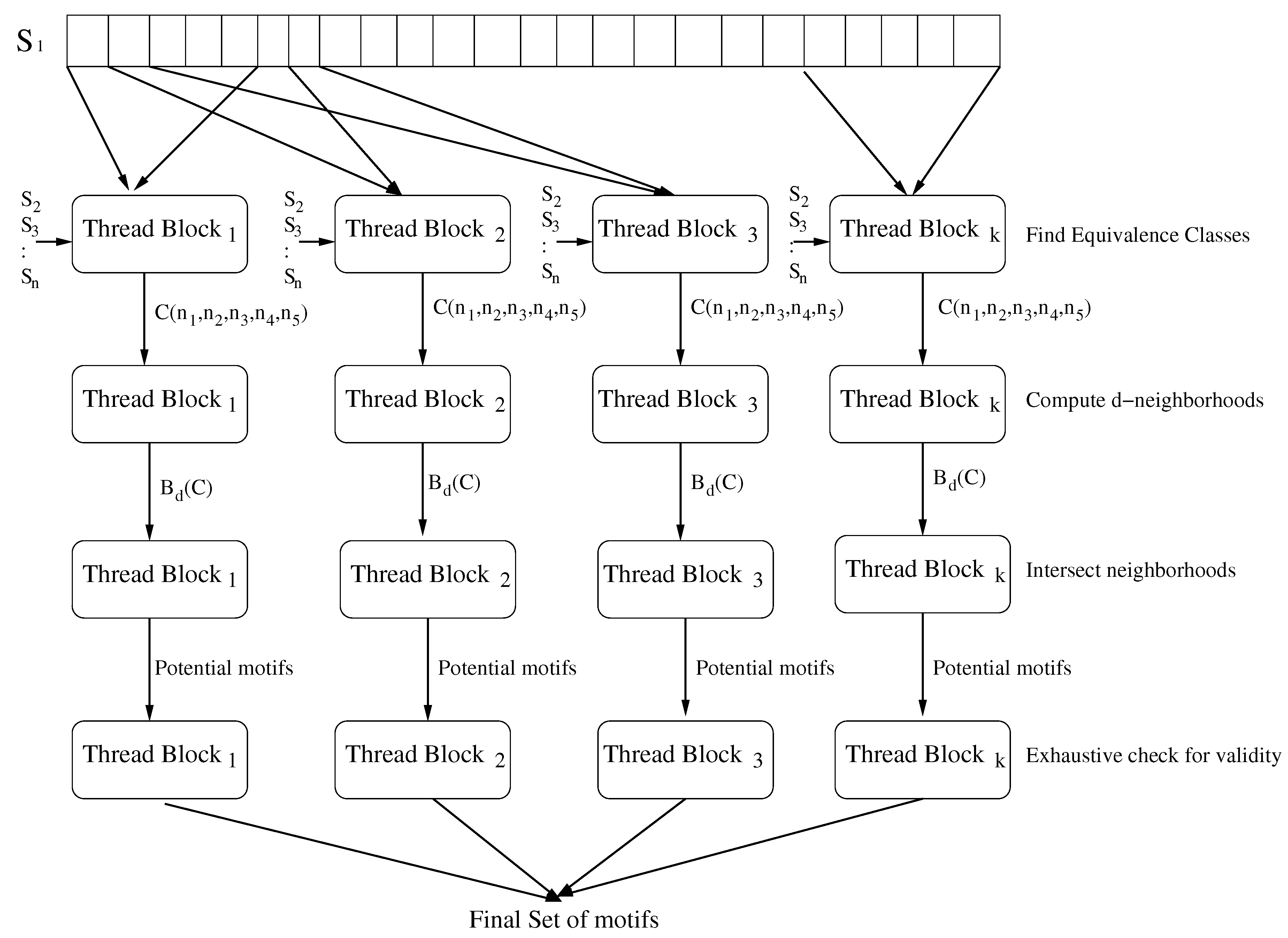
The preceding strategy to generate generates l-mers w for each 10-tuple . While every generated l-mer is in , some l-mers may be the same. Computational efficiency is obtained by computing for all in the same class concurrently by sharing the loop overheads as the same loops are needed for all in a class. Algorithm 2 gives the pseudocode to compute by classes.
As an example, lets say we have 3 input strings , and and we are asked to find motifs i.e., motifs of length 3 with at most 1 mismatch. Also, the l-mer is denote by . In this particular case, and hence for example. For the triplet , i.e., for the triplet we have . Hence it belongs to the class . For the triplet i.e., we have and it belongs to class . After evaluating all 8 triplets, we will end up having class . We then need to find and to compute . To computer , we need to compute . We can evaluate that , and and subsequently we have . Similarly, we can see that and hence . Run-time may be reduced by pre-computing data that do not depend on the string set S. So, for a given pair , there are 5-tuples . For each of the 5-tuples, we can pre-compute all 10-tuples () that are solutions to the ILP. For each 10-tuple, we can pre-compute all combinations (i.e., selections of positions in w). The pre-computed 10-tuple solutions for each 5-tuple are stored in a table with entries and indexed by and the pre-computed combinations for the 10-tuple solutions are stored in a separate table. By storing the combinations in a separate table, we can ensure that each is stored only once even though the same combination may be needed by many 10-tuple solutions.
| Algorithm 2: Compute [23]. |
ClassBd()
Find all ILP solutions with parameters
for each solution ()
{
← first combination for this solution;
for i = 0 to (# combinations)
{
for each triplet in
{
Generate ws for ;
Add these ws to ;
}
← next combination in Gray code order;
}
}
return
|
We store pre-computed combinations as vectors. For example, a Type 1 combination for and could be stored as indicating that the first and third Type 1 positions of w have a character different from what x, y, and z have in that position while the character in the second Type 1 position is the same as in the corresponding position of x, y, and z. A Type 2 combination for and could be stored as indicating that the character in the first Type 2 position of w comes from the third l-mer, z, of the triplet, the second Type 2 position of w has a character that is different from any of the characters in the same position of x and z and the third and fourth Type 2 positions of w have the same character as in the corresponding positions of x. Combinations for the remaining position types are stored similarly. As indicated by our pseudocode of Algorithm 2, combinations are considered in Gray code order so that only two positions in the l-mer being generated change from the previously generated l-mer. Consequently, we need less space to store the combinations in the combination table and less time to generate the new l-mer. An example of a sequence of combinations in Gray code order for Type 2 positions with is {0012, 0021,0120,0102,0201,0210,1200,1002,1020, 2010, 2001, 2100}. Note that in going from one combination to the next only two positions are swapped.
2.4. The Data Structure Q
We now describe the data structure
Q that is used by PMS6. This is a reasonably simple data structure that has efficient mechanisms for storing and intersection. In the PMS6 implementation of [
23], there are three arrays in
Q; a character array,
, for storing all
l-mers, an array of pointers,
,which points to locations in the character array and a bit array,
, used for intersection. There is also a parameter
which determines how many characters of
l-mers are used for indexing into
array. As there are 4 possibilities for a character, for
p characters
can vary from 0 to
. The number of characters,
p, to be used for indexing into
, is set when
Q is initialized. During the first iteration of PMS6, for
,
l-mers in
are stored in
. After all
s are computed,
is sorted in-place using Most Significant Digit radix sort. After sorting, duplicate
l-mers are adjacent to each other. Also,
l-mers that have the same first
p characters and hence are in the same bucket are adjacent to each other as well in
. By a single scan through
, duplicates are removed and the pointers in
are set to point to different buckets in
. During the remaining iterations, for
, all
s generated are to be intersected with
Q. This is done by using the bit array
. First, while computing
, each
l-mer is searched for in
Q. The search proceeds by first mapping the first
p characters of the
l-mer to the corresponding bucket and then doing a binary search inside
within the region pointed to by the bucket pointer. If the
l-mer is found, its position is set in
. Once all
l-mers are marked in the
,
is compacted by removing the unmarked
l-mers by a single scan through the array. The bucket pointers are also updated during this scan.
For larger instances, the size of
is such that we don’t have sufficient memory to store
in
Q. For these larger instances, in the
iteration, we initialize a Bloom filter using the
l-mers in
rather than storing these
l-mers in
Q. During the next iteration (
k = 2), we store, in
Q, only those
l-mers that pass the Bloom filter test (
i.e., the Bloom filter’s response is “Maybe"). For the remaining iterations, we do the intersection as for the case of small instances. Using a Bloom filter in this way reduces the number of
l-mers to be stored in
Q at the expense of not doing intersection for the second iteration. Hence at the end of the second iteration, we have a superset of
(Algorithm 1) of the set we would have had using the strategy for small instances. Experimentally, it was determined that the Bloom filter strategy improves performance for challenging instances of size (19,7) and larger. As in [
22], PMS6 uses a partitioned Bloom filter of total size 1GB. From Bloom filter theory [
26] we can determine the number of hash functions to use to minimize the filter error. However, we need to minimize the run time rather than the filter error. Experimentally, [
23] determined that the best performance was achieved using two hash functions with the first one being bytes 0–3 of the key and the second being the product of bytes 0–3 and the remaining bytes (byte 4 for (19,7) instances and bytes 4 and 5 for (21,8) and (23,9)instances).


