1. Introduction
A networked control system (NCS) is a fully-distributed and networked real-time feedback control system between sensors, actuators and controller signals transmitted over the network [
1]. The communication network in the feedback control loop introduces a significant additional delay, especially in complex networks [
2]. The time delay can be constant or time varying, which makes the analysis and control design more complex [
3]. For the network-induced time-delay compensation problem, many scholars have conducted a great deal of research work. Robust control [
4,
5], intelligent control [
6,
7], predictive control [
8,
9], pinning control [
10–
12] and other time-delay compensation methods have led to a lot of developments and applications.
Generalized predictive control (GPC) was proposed by Clarke in 1987. GPC has many advantages: the first one is based on the parameters of the model; secondly, it retains the advantage of adaptive control and has better robustness than adaptive control; finally, due to the adoption of multi-step prediction, rolling optimization and the feedback correction strategy, the control effect is more suitable for industrial process control requirements.
The auto regression model is utilized to predict the time delay, and an improved GPC algorithm for time-delay compensation was proposed [
13]; however, the author did not give the details of the simulation parameters. Based on a random time-varying network delay, the GPC network based on a state space model is used to access an effective tracking performance [
14]. Liu
et al. gives a predictive control method for a forward channel and feedback channel with random time delay and gives the closed-loop predictive control system stable conditions [
15]. However, the GPC algorithm requires solved Diophantine equations and a matrix inversion operation, which led to excessive online calculation; on the other hand, since the time delay is random, the parameter selection for the GPC algorithm requires a larger prediction step size, thereby increasing the calculation time. Furthermore because the network delay is uncertain, the GPC algorithm requires a larger prediction step, thus increasing the computing time, reducing the real-time performance of the system [
16].
Based on the above analysis, the research motivation of this paper includes two aspects. The first is to find a suitable predictive method to predict time delay, to reduce the prediction step size of the GPC algorithm. The second is to improve the GPC algorithm, reducing the calculation amount of the GPC algorithm. This paper will carry out research work on these two aspects. In the literature [
17], the author used the particle swarm optimization (PSO) algorithm optimized least squares support vector machine (LS-SVM) to predict the future time delay, compensating time delay through implicit GPC, but the embedding dimension is not optimized in the paper. At the same time, the control value of implicit GPC needs to wait for the next integer time sampling period to be applied to the controlled object. It is easy to cause the system response speed to slow and to produce a big overshoot, so it is necessary to improve it. On the basis of the literature [
17], this paper discussed LS-SVM prediction accuracy with different parameters, firstly using the genetic algorithm-optimized parameters of the LS-SVM time-delay prediction model, and then, an improved implicit generalized predictive control method is used to compensate for the random time delay; the output performance of the system is improved. Through the simulation, the effectiveness of the proposed method in this paper is verified.
2. LS-SVM Time-Delay Prediction Model
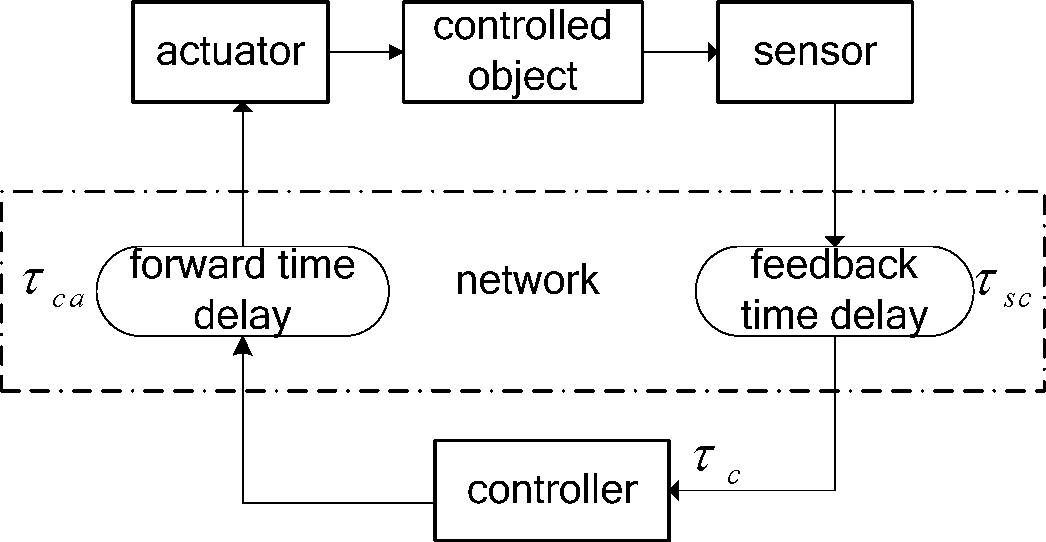
The time delay in the networked control system includes: the sensor for the controller time delay τ
sc, the controller to the actuator time delay τ
ca and the controller calculated time delay τ
c, shown as in
Figure 1.
The sensor for the controller time delay and the controller to actuator time delay do not have the same variation rules, and the effect on the system performances is not the same either. Under normal circumstances at time
k, the sensor to the controller time delay τ
sc(
k) can be measured, and the controller to actuator time delay τ
ca (
k) and controller computing time τ
c(
k) are unknown, but just moments before
k is known, so the historical time delay can be used to predict the current network time delay. In the networked control system discussed in this paper, the controller and actuator are event driven, and the sensor is clock-driven; therefore, the forward and feedback channel time delay of networked control system can be combined for analysis [
13]. The system total delay can be expressed as τ(
k) = τ
ca (
k) + τ
sc (
k) + τ
c (
k). Because the time delay can be combined for analysis, the total system time delay
τ(
k) can be predicted through an appropriate prediction model.
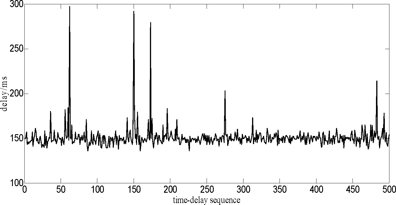
Figure 2 gives 500 groups’ time delay test data collected from an IEEE 802.11b-based networked control system. From the figure, it can be seen that time delay has a strong, nonlinear characteristic, and the mean value of the time delay sequence is within a range of variation over a longer time, but, in a certain interval during a shorter time.
The predictability and similarity of the time-delay sequence can be measured by the Hurst parameter; the time-delay sequence has self-similarity when
H ∈ (0.5,1); the greater
H is, the greater is the sequence similarity. In this paper, the
R/
S (rescaled range analysis) method is used to calculate the Hurst parameter of the time-delay sequence, and it can be described as:
where in
n is the number of samples,
R is the rescaling range, that is
R = max(
Xt,n −min
Xt,n),
t = 1,2,…,
n,
S is the standard deviation,
H is the Hurst parameter and
A is a constant. Given the chart of the relationship between lg(
R/
S)
n about lg
n, the least squares method is used for calculating the slope, and then, the slope is Hurst parameter.
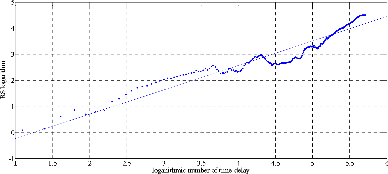
The Hurst parameter of the time-delay sequence is commutated by the
R/
S method, as shown in
Figure 3. Using a straight line linear fitting of these data points, the slope of the line is the Hurst parameter,
H is 0.936, apparently satisfying 0.5 <
H <1, which also shows that the time-delay sequence has self-similarity. Therefore, the time-delay sequence can be predicted through the LS-SVM model.
The standard SVM algorithm is complex; based on the standard SVM, LS-SVM sets the loss function of SVM as square errors, converts the inequality constraints into equality constraints and reduces the undetermined parameters. At the same time, it transforms the quadratic programming problem into linear equations, which can reduce the complexity of the solution [
17].
LS-SVM uses the following function to estimate the random time delay of the networked control system [
18]:
Nonlinear function
Φ(·) can transform the input space to a high dimensional feature space, so that the nonlinear fitting of input space can be seen as a linear fitting of the high dimensional feature space. Let {
xi,
yi},
i = 1, 2,⋯,
N be a training set, based on the risk minimization principle; the regression problem can be expressed as a constrained optimization problem:
Wherein
xi is a time-delay input set,
yi is a time-delay output prediction set,
xi and
yi can be expressed as
xi =[
di di+1 ⋯
di+m−1],
yi = [
di+m] and
m is the embedding dimension; and the current time and past
m − 1 time-delay value can be used to predict the next time-delay value of the system.
λ is the regularization parameter.
b is the constant value deviation. The Lagrange function can be established to solve the above optimization problem:
ai is the Lagrange multiplier. Calculate the partial differential of
w,
b,
e,
a, and simplify it; then, the next equation can be obtained:
For the given training set {
xi,yi},
Equation (6) is used to calculate parameters
a and
b, at the same time. When the given set
x combines with the actual training set
xi, the following equation can be used to calculate
y, the prediction output of the system.
In this paper, the radial basis function (RBF) is chosen as the kernel function of LS-SVM, it is:
From the above modeling process, based on the kernel function of RBF, LS-SVM performance depends mainly on γ and σ
2, but the selection of two parameters lacks uniform standards and theoretical guidance; therefore, the selection of LS-SVM parameters is an unsolved problem [
19]. At the same time, for the time-delay prediction problem, the embedding dimension
m is an important parameter also;
m that is too small will reduce the prediction accuracy;
m that is too large will increase the computational complexity. The following
Tables 1–
3 give the mean square error (MSE) comparison of three different values of the parameters.
From the above data in the Tables, three parameters can greatly affect the prediction accuracy, and only optimizing a parameter separately cannot guarantee that the other parameters are optimal, leading to the prediction precision being not ideal. In order to obtain the best prediction results, it is necessary to make m, γ, σ2 achieve the optimal values at the same time.
3. Genetic Algorithm
The genetic algorithm (GA) uses the biological genetics view, through natural selection, exchange, mutation operation,
etc. Through the population, evolution is carried out, and it has a strong global search ability and can obtain the global optimal solution in a relatively short time [
20].
3.1. Individual Coding
The LS-SVM time-delay prediction model needs the parameters
m, γ and σ
2. The individual design is shown in
Figure 4: the former
n1 bits represent
m; the middle
n2 bits represent γ; the later
n3 bits represent σ
2.
Each of the individual can convert a binary classification string into decimal representation as the actual parameters:
In the above equation, p is the parameters decimal value, min(p) is the parameters minimum, max(p) is the parameters maximum value, k is the length of the parameters binary string, d is the decimal value of the parameters binary string.
3.2. Population Initialization
The standard GA algorithm initial population is random, has a lot of uncertainty and no uniformity, and it cannot contain the global optimal solution information, so leading to the local optimal problem; thus, in this paper, uniform design is used to produce the initial population to ensure the diversity of the initial population and the uniformity of the individual step distribution [
21].
3.3. Fitness Function
The GA algorithm search target is to find the appropriate
m, γ, σ
2, so that it can improve the prediction precision of the delay; thus, the fitness function is related to the accuracy of the time-delay prediction model. Set the
i-th group time-delay prediction mean square error as:
In the above equation,
n is the number of the time-delay sequence,
yi is the actual value and
is the LS-SVM prediction value of the
i-th time-delay. For easy calculating, the
i-th prediction time-delay fitness function directly uses the mean square error:
3.4. The Design of the Genetic Operator
For the selection operators, calculate the individual fitness value and order the fitness from big to small; the smaller fitness shows a smaller error; thus, it is the best individual. Use that individual to keep the strategy, and choose the R-th optimal individuals as the next generation. The other n − R individual crossover and mutation operation produces a new individual as the next generation.
For the crossover operator, in the individuals, three parts separately select three intersections; then, the crossover operator can respond to the part of another individual. After this, test the generated individual, and verify whether the choice of parameters is in a certain range; if not, repeat the crossover operation again.
For the mutation operator, for the three parts of an individual, adopt the traditional flip variation method on the variation operation, and randomly select one individual bit, according to the rules that convert zero to one and one to zero. Carry out the variation operation, and then, test whether the individual variation is in the parameter range; if not, repeat the crossover operation again.
3.5. GA Optimized LS-SVM Time-Delay Prediction Method
To sum up, the GA-optimized LS-SVM time-delay prediction method steps are:
Step 1: Confirm the original character space of the optimized parameters, and the initial evolution algebra is zero.
Step 2: Code the parameters m, γ, σ2.
Step 3: Generate h individual initial populations.
Step 4: Convert the time-delay sequence, which is the original length, into the input and output matrix, according to xi=[di di+1 ⋯ di+m−1], yi=[di+m] The LS-SVM algorithm is used to train and predict according to the parameters γ, σ2, recording every group time-delay prediction accuracy and each individual fitness value.
Step 5: Choose the best R prediction performance individual for the next generation, and for the other individual, carry out the selection, crossover and mutation operators, producing a new population. The evolution algebra is increased one.
Step 6: Judge whether this meets the end conditions, and if it meets them, jump to Step 7 or return to Step 4 otherwise.
Step 7: Output the best individual m, γ, σ2, and adopt the optimum m, γ, σ2 as the LS-SVM algorithm parameters to build up the time-delay prediction model. Output the best prediction value.
4. Improved Implicit GPC Time-Delay Compensation Algorithm
Set the total time delay between the controller and actuator, sensor and controller in the NCS as
d(
k). The NCS can be expressed as an auto-regression and moving average with exogenous (ARMAX) model with time-varying discrete parameters:
wherein:
dmin ≤
d(
k) ≤
dmax is the whole time-delay of the NCS;
u(
k) is the input;
y(
k) is the output;
v(
k) is the interference; and
ai(
k),
bi(
k),
ci(
k) are the time-varying parameters of the system.
4.1. The Identification of the Time-Varying Parameters
After the random time delay has been predicted through the LS-SVM algorithm, the networked control system can be written as a regression model.
Then, the next equations can be obtained:
In the above equations, r is the forgetting factor, 0 ≤ r ≤ 1; the initial value, P(0) = δ2I, θ(0) = 0, δ2 is a sufficiently large constant and I is the unit matrix. Through the above method, the time-varying parameters ai(k), bi(k), ci(k) of the system can be identified.
4.2. Improved Implicit GPC
Scroll the optimization to make the objective function minimum:
In the equation,
E is the mathematical expectation,
P is the maximum prediction length,
M is the control length,
M ≤
P, λ are the weighting coefficients, Δ
u(
k+
j−1) is the control increment and
yr(
k +
j) is the input reference trajectory. The GPC algorithm calculates
y(
k +
j), needed to solve the Diophantine equation. To avoid complex calculation, an improved implicit GPC algorithm is presented in this paper. This algorithm directly identifies the controller parameters and does not need to solve the inverse matrix of the GPC algorithm. The algorithm, given the
dth optimal prediction value, is:
Define the input soft coefficient β as:
The above equation can prevent input signal intensity changes, and it also restricts the change of the input signal. The control increment value matrix is:
Rewrite
Equation (18) of the performance index as the vector form:
Due to the existence of the soft change matrix, it can be seen that no matter how the length of the predictive domain changed, the control value always is Δu(k). Secondly, the calculation of the inverse matrix is avoided, greatly reducing the calculation time and ensuring the speediness of the system. However, the algorithm still retains the basic characteristics of the generalized predictive control.
In order to accelerate the response speed of the system and to restrain overshooting, this paper proposed an improved implicit GPC algorithm. The next step control increment value is used for the compensation of
Equation (26), and the real control value can be obtained as:
The above equation is equivalent to an increase of the differential effects on control system; it will accelerate the response speed of the system.
Since the improved implicit GPC algorithm is used in the controller, so the control value sequence of the future N cycles (N is the length of the control sequence) at time k can be calculated, but the specific use of the control sequence that acts on the actuator can be determined according to the relationship between the time delay and the sampling period.
Assuming that the system sampling period is
T, the time delay of the current control cycle is τ. Let:
Select u(k + n | k) as the current control value. Therefore, after a delay of τ, the control value is acting on the controlled object at the k + n moment; the control system with time delay is transformed into a control system without time delay.
The improved implicit GPC time-delay compensation steps of this paper can be expressed as follows:
Step 1: Set the initial value.
Step 2: Update the input time-delay sequence, and put the newest measurement of the time delay into the time-delay sequence.
Step 3: The GA-optimized LS-SVM algorithm is used to estimate the network time delay at the current time.
Step 4: Identify time-varying parameters through the prediction time delay by
Equations (16) and
(17).
Step 7: According to
Equation (32), the control value
u(
k + n |
k) is calculated and sent to the actuator;
Step 8: Repeat Step 2 to Step 7 until the end of the simulation.
5. Simulation
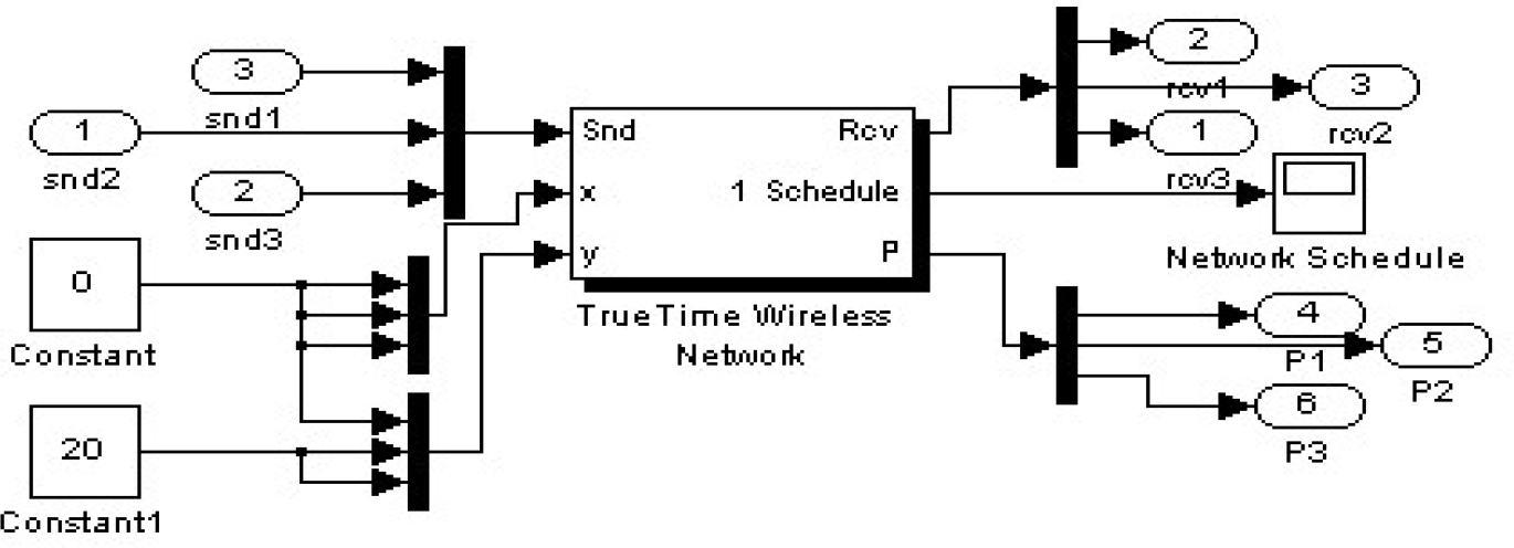
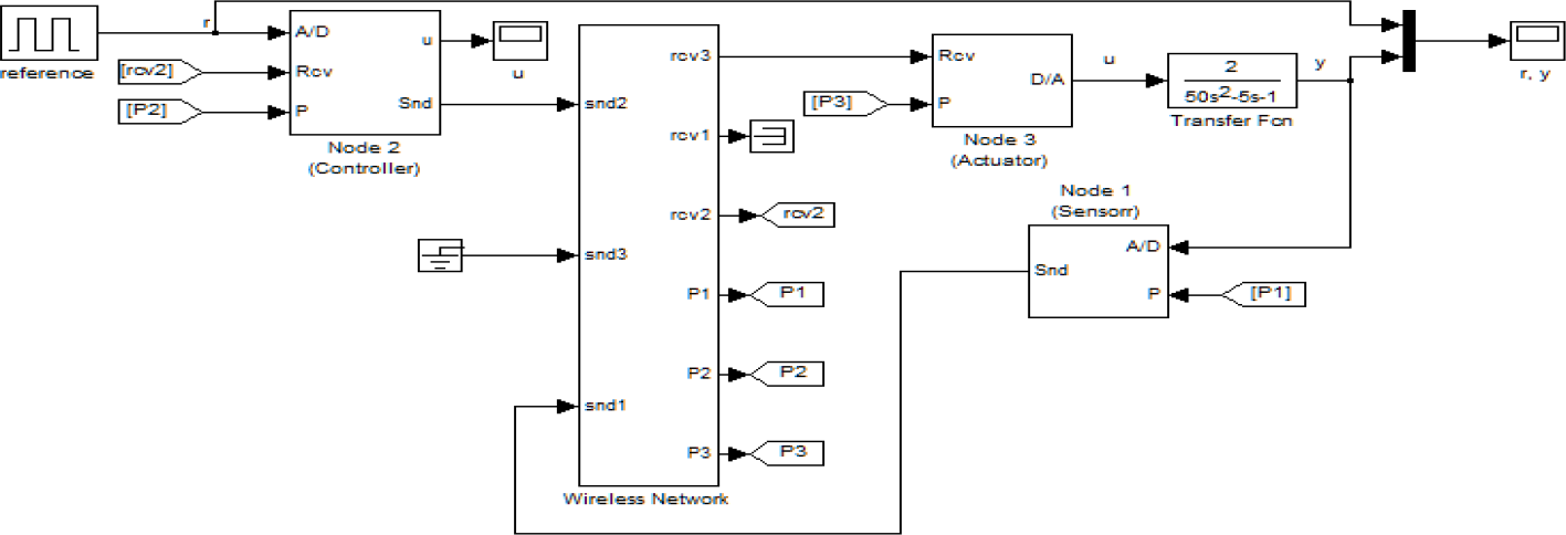
The true time toolbox is used to build an IEEE 802.11b wireless NCS. Sensors are time driven, and controllers and actuators are event driven. The sampling period is 10 ms; the network speed is 80,000 bits/s; the minimum frame size is 80 bits; the packet size is 80 bits. The interfering node is added to the system; the interference ratio is 10%; and the interference can create the network time-delay random variation. An unstable controlled object is chosen as:
The structure of the IEEE 802.11b network is as shown in
Figure 5. The whole simulation structure is as shown in
Figure 6. In these figures, Snd means send node, Rcv means receive node.
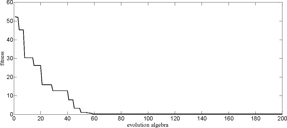
Then, 300 groups’ time-delay test data are collected, and the first 200 groups’ data are used to train the GA-optimized LS-SVM time-delay prediction model. The last 100 groups’ data are used to verify it. GA algorithm parameters: the number of iterative evolutions is 200; the population quantity is 20; the crossover probability is 0.9; the variation probability is 0.1; the coding length of
m, γ, σ
2 is 10 bits; the
m value range is from one to 20; the γ value range is from 0.01 to 1000; the σ
2 value is range from 0.01 to 100; after GA optimized,
m = 9, γ = 339.8592 and σ
2 = 2.347; the MSE is 1.26 for the actual and predicted time delay.
Figure 7 is the curve of fitness.
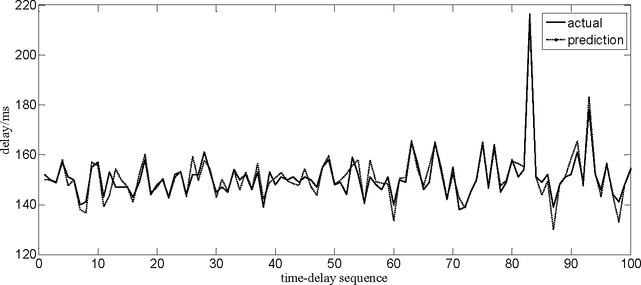
Figure 8 is a 100 groups’ comparison of the predicted and actual time delay.
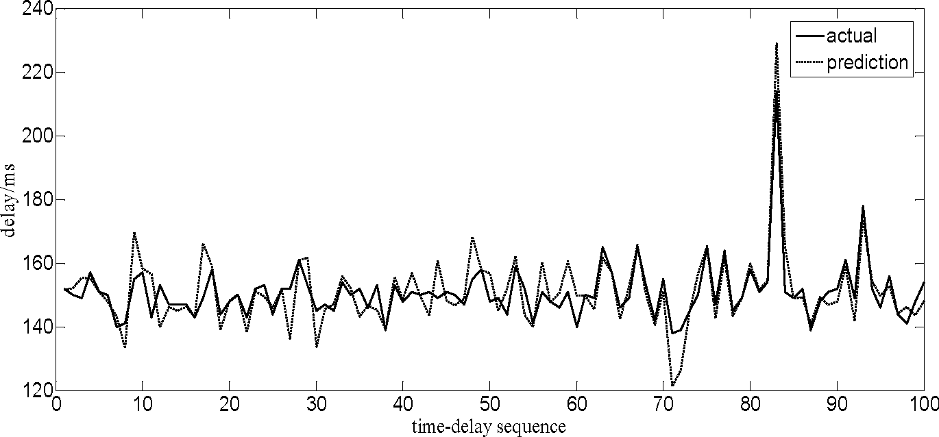
Figure 9 shows the comparison of the predicted and actual time delay with auto regression (AR) algorithm in the literature [
13]; the order of
p is nine; the MSE is 10.2791 for the actual and predicted time delay. From the contrast in
Figure 8,
Figure 9 and the MSE, it can be shown that the time-delay prediction precision of the GA-optimized LS-SVM prediction method is better than the AR algorithm in the literature [
13].
In order to verify the time-delay compensation ability of the improved implicit GPC control algorithm, the simulation is conducted through the built IEEE 802.11b wireless NCS. The improved implicit GPC parameters of the control algorithm are
P = 6,
M = 6, β = 0.2, ∂ = 0.1. A comparison of the method in the literature [
17] is shown in
Figure 10 for the square-wave tracking and in
Figure 11 for the square-wave tracking with an added white noise amplitude of 0.2 at the output.
The simulation results show that the GA optimized LS-SVM time-delay prediction with improved implicit GPC time-delay compensation method is better than the method in literature [
17] in overshoot and response time; it can better track system input and ensure the stability of the system.
A measured control cycle needs 3.4 ms for the method in the literature [
17] and 2.1 for the method in this paper. The results showed that the method in this paper is about 1.61-times faster than the method in the literature [
17]. Therefore, the method in this paper enhances the time-delay compensation capability and does not increase the execution time; therefore, it is more suitable for the time-delay compensation of a networked control system.
6. Conclusions
In the network control system, uncertain factors, such as network delays, can usually deteriorate the control performance and stability of networked control systems. Therefore, a time-delay compensation method based on time-delay prediction and improved implicit GPC is proposed. First, the GA-optimized LS-SVM prediction model is used to estimate the time delay in the networked control system. Then, an improved implicit GPC with predictive time delay is used to obtain the system future control value, to compensate for the time delay of the networked control system. Finally, through the simulation results, the method presented in the paper has a better compensation effect and a smaller calculation time.
In this paper, the parameters of the LS-SVM prediction model are optimized by the genetic algorithm off-line. Additionally, if the time-delay sequence appears to have substantial changes, the prediction accuracy will be reduced. Therefore, the future work is to increase the threshold value; when the cumulative error is larger than the threshold, the optimization process of the parameters is repeated, and more appropriate prediction parameters can be obtained.


