1. Introduction
A large number of problems in science and engineering require the solution of a nonlinear equation
f(
z) = 0. There are different techniques to tackle this problem, and one of the most commonly used is the numerical solution with iterative methods. The Newton’s method is a well-known iterative scheme to estimate the solution of nonlinear equations
However, in many situations it is not possible to evaluate the derivative. In Section 2, several optimal derivative-free methods, with increasing orders of convergence, are introduced, in order to avoid the evaluation of the derivative.
The efficiency index, introduced by Ostrowski (see [
1]), feeds back the comparison between methods in terms of efficiency. It is defined as
I =
p1/d, where
p is the order of convergence and
d is the number of functional evaluations per step. A method is optimal if
p = 2
d−1, as Kung and Traub conjectured in [
2].
The quality of an iterative method can be measured by distinct parameters, as the efficiency index, the order of convergence, …, but the stability is a capital element that needs to be analyzed. The dynamical planes of the iterative schemes supply this information graphically, and are developed in Section 3. Several authors have studied and compared the stability of different known iterative methods by means of their dynamical planes, firstly in the work of Varona [
3] and later on developed by Amat
et al. [
4], Neta
et al. [
5,
6], among others.
The dynamical behavior of Newton’s method on polynomials, as studied in [
7,
8] among others, shows that its stability is not guaranteed in the whole dynamical plane. Finding the fractal dimension of an iterative method is a technique to measure this Julia set and, therefore, a useful tool to characterize the stability of a method. In Section 4, the fractal dimension of the introduced methods is evaluated.
In this paper, we analyze the dynamical behavior of four derivative-free schemes, with orders of convergence 2, 4, 8 and 16, on different quadratic and cubic polynomials. From this analysis, some results can be conjectured. For example, the Julia sets of the corresponding rational functions have less complexity and the basins of attraction obtained by the different schemes are wider, becoming more similar to that of Newton’s method, as the order of convergence increases. From a numerical point of view, these facts are checked by the fractal dimension of each procedure, that gets increasingly close to Newton’s one.
2. Optimal Derivative-Free Methods
The well-known Steffensen’s method (see [
9]) replaces the derivative of
Equation (1) by the forward difference, so its iterative expression is
where
vn =
zn +
f(
zn). The composition technique (described, for instance, in [
10]) allows up the implementation of high-order methods. From two methods with orders of convergence
p1 and
p2 is possible to perform a method of
p1 ·
p2 order. In [
11], the authors describe a technique based on composition and Padé-like approximants to obtain optimal derivative-free methods.
We first compose Steffensen’s method with Newton’s scheme obtaining the fourth-order scheme
where
vn =
zn +
f(
zn). Now, in order to avoid the evaluation of
f′(
yn), we approximate it by the derivative
m′(
yn) of the following first degree Padé-like approximant
where
a1,
a2 and
a3 are real parameters to be determined satisfying the following conditions:
and
Conditions (
4) and (
6), give, respectively,
and
where
f[
zn, yn] denotes the divided difference
. After some algebraic manipulations, the following values are obtained for the parameters:
and
where
is a second order divided difference.
The derivative of the Padé approximant evaluated in
yn can be expressed as
Substituting
f′(
yn) from
Equation (3) by its approximation
m′(
yn), Cordero
et al. in [
11] obtained an optimal fourth-order iterative method denoted by M4, whose expression is:
By composing again the resulting scheme with Newton’s method, and estimating the last derivative by a Padé-like approximant of order two, the obtained optimal eighth-order method, denoted by M8, has the iterative scheme
In a similar way, we can obtain a new optimal 16th-order method, denoted by M16, by composing the scheme M8 with Newton’s method and estimating the last derivative by a Padé-like approximant of third degree
obtaining the iterative expression
where
,
c4 =
f [
zn;
yn;
vn;
wn] +
c5f [
zn;
yn;
vn],
c3 =
f [
zn;
yn;
wn] −
c4(
zn +
yn − 2
wn) +
c5f [
zn;
yn]and
f [
·, ·, ·, ·] and
f [
·, ·, ·, ·, ·] are the divided differences of order three and four, respectively.
This procedure can be extended in order to obtain optimal derivative-free iterative schemes with convergence order 2k−1, k = 2, 3, 4, 5, …. All the methods designed in this way are optimal in the sense of Kung-Traub’s conjecture, since the methods of order 2k−1 need k functional evaluation per iteration, k = 2, 3, …
3. Complex Dynamics of Iterative Methods
The dynamical planes provides an at-a-glance status of the convergence and stability of a method. In this section, the dynamical planes of the introduced methods are shown. In order to get a better understanding, some dynamical concepts are recalled. For a more extensive and comprehensive review of these concepts, see for example [
7,
8].
Let R : Ĉ → Ĉ be a rational function, where Ĉ is the Riemann sphere. The orbit of a point z0 ∈ Ĉ is defined as {z0, R(z0), …, Rn(z0), …}.
The dynamical behavior of the orbit of a point on the complex plane can be classified depending on its asymptotic behavior. In this way, a point z0 ∈ C is a fixed point of R if R(z0) = z0. A fixed point is attracting, repelling or neutral if |R′(z0)| is less than, greater than or equal to 1, respectively. Moreover, if |R′(z0)| = 0, the fixed point is superattracting.
Let
be an attracting fixed point of the rational function R. Its basin of attraction
is defined as the set of pre-images of any order such that
. In our calculations, we usually consider the region [−5, 5] × [−5, 5] of the complex plane, with 600 × 600 points and we apply the corresponding iterative method starting in every z0 in this area. If the sequence generated by iterative method reaches a zero z* of the polynomial with a tolerance |zk – z*| < 10−3 and a maximum of 40 iterations, we decide that z0 is in the basin of attraction of these zero and we paint this point in a color previously selected for this root. In the same basin of attraction, the number of iterations needed to achieve the solution is showed in darker or brighter colors (the less iterations, the brighter color). Black color denotes lack of convergence to any of the roots (with the maximum of iterations established) or convergence to the infinity.
The set of points whose orbits tends to an attracting fixed point (or an attracting periodic orbit)
is defined as the Fatou set,
. The complementary set, the Julia set
, is the closure of the set consisting of its repelling fixed points, and establishes the boundaries between the basins of attraction.
If the rational function R is associated to the fixed point operator of the developed methods in Section 2 applied on a polynomial f(z), denoted generically as Of(z), it is possible to find its fixed and critical points. The fixed points zf verify Of(z) = z, and the critical points zc validate
.
The expressions
where
v =
z +
f(
z),
y =
Sf(
z),
u =
Ff(
z) and
w =
Ef(
z), are the fixed point operators of Steffensen’s, M4, M8 and M16 methods, respectively.
From the dynamical point of view, conjugacy classes play an important role in the understanding of the behavior of classes of maps in the following sense. Let us consider a map z → Mf(z) whose Mf is any iterative root-finding map. Since a conjugacy preserves fixed and periodic points, as well as their basins of attraction, the dynamical information concerning f is carried by the character of the fixed points of Mf. So, for polynomials p of degree greater than or equal to k, it is interesting to build up parametrized families of polynomial pµ, as simple as possible, so that there exist a conjugacy between Mpµ and Mp.
In order to study affine conjugacy classes of an iterative method
Mf, we need to establish a result that is is called Scaling Theorem. As the authors proved in [
12], Steffensen’s method does not satisfy the Scaling Theorem, and this statement can be proved in a similar way for M4, M8 and M16. Then, these schemes have not conjugacy classes and we must study their dynamics on specific polynomials. The behavior of each method is analyzed on four different polynomials:
pc (
z) =
z2 +
c and
qc (
z) =
z3 +
c, where
c ∈ {1,
i}. The introduced fixed point operators satisfy the symmetry property
, ∀
c, z ∈ C. Consequently, for polynomials with
c ∈
R, the dynamical planes are symmetric respect to the abscissas axis. For polynomials with
c ∈
C, the dynamical planes of
are a vertical reflection of
. Therefore, the study of
pc(
z) and
qc(
z), with
c ∈ {1,
i}, directly involves the knowledge of
c ∈ {
−1,
−i}.
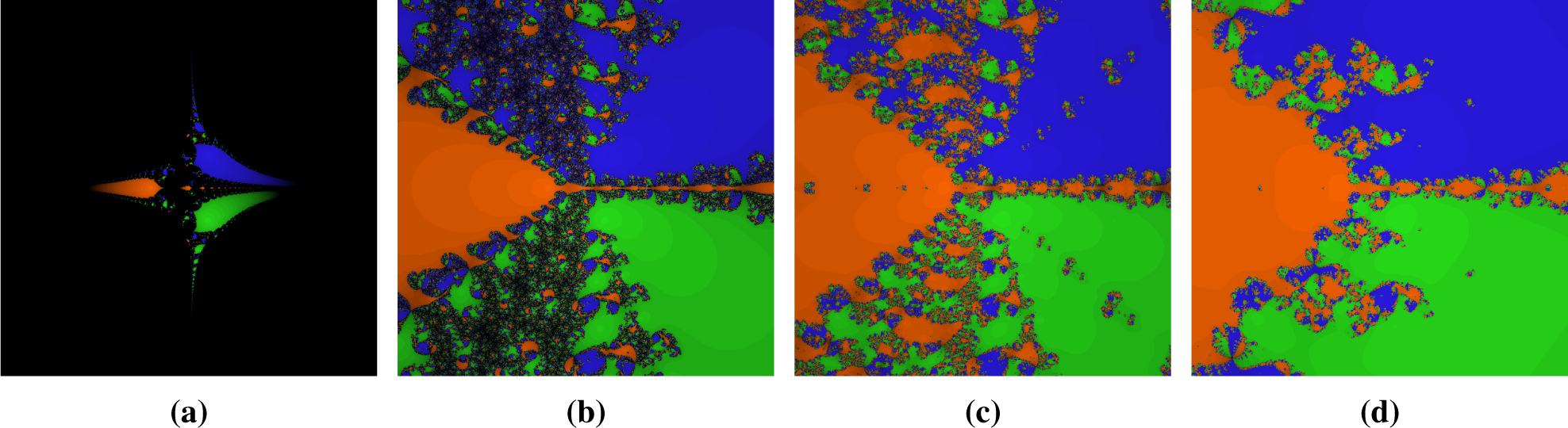
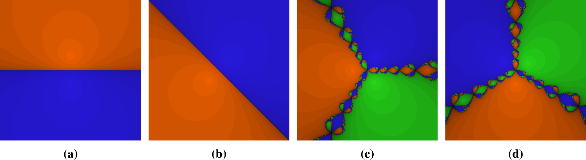
The dynamical planes of
Sf(
z),
Ff(
z),
Ef(
z) and
Xf(
z), when they are applied to
p{1,i}(
z) and
q{1,i}(
z), are displayed in
Figures 1–
4. The basins of attraction are colored in orange and blue—for quadratic polynomials—and also in green—for cubic polynomials. The black points are those that do not converge to any of the attracting fixed points. We observe that the basins of attraction get wider when the order of convergence is increased, obtaining fast convergence in regions of initial guesses where the original scheme is divergent. A reason for this behavior can be found in [
12], where the authors prove that the infinity is an attracting fixed point of Steffensen’s method, and it is repulsive in case of M4 (in a similar way, it can be checked that it is also repulsive for M8 and M16).
As
Figures 1–
4 show, except for Steffensen’s method, the complexity of the dynamical planes gets smoother as the order of convergence increases.
The dynamical planes of the fixed point operator associated to Newton’s method,
Nf(
z), when it is applied to
pc(
z) =
z2 +
c and
qc(
z) =
z3 +
c, with
c ∈ {1,
i}, are shown in
Figure 5.
If we focus on the evolution of M4 to M16, passing through M8, it is observed that they are closer to the Newton’s dynamical planes, for each polynomial.
4. Fractal Dimension of Iterative Methods
The fractal dimension of the Julia set is a useful tool to analyze how close is a dynamical plane to another. Usually, the fractal dimension is obtained by the box-counting algorithm, based on the Hausdorff dimension. The foundations of this algorithm (see, for instance, [
13]) goes by covering the Julia set by boxes small and smaller, in order to find
where
ϵ is the length of the boxes,
N(
ϵ) is the account of boxes that cover the Julia set, and
D is the fractal dimension. Computationally, the value of
D is obtained as the slope of the regression line of log
ϵ vs. log
N(
ϵ).
Table 1 gathers the fractal dimension of operators (
12), (
13), (
14) and
Nf(
z) when they are applied to the previously submitted polynomials in the top rows. The comparison of each method to Newton’s one is made by the percentage of their fractal dimension, shown in bottom rows.
Graphically, we observe that the dynamical plane of the different methods on an specific polynomial “tends” to the corresponding dynamical plane of Newton’s one. We can see, for example, in
Figure 4, how the different pictures are looking increasingly to
Figure 5d. Also, the Julia sets have less complexity as the order of convergence increases. In a numerical sense, taking into account the fractal dimension of each method, it gets close and closer from Newton’s one.
There are some studies about the fractal dimension of Newton’s dynamical plane. For instance, in [
14] the fractal dimension of
Nqc(
z), with
c =
−1, is
D = 1.44692 in the square [
−2.5, 2.5]
× [
−2.5, 2.5], whereas our calculus in this region gets
D = 1.4055. Also, in [
15], in the square [
−1, 1]
× [
−1, 1],
D ≈ 1.42, while in our study, the value of the fractal dimension in this square is
D = 1.4242. The exact value depends on the details of the algorithm, such as the thickness of the Julia set or the chosen sequence of
ϵ. However, our purpose is the comparison of the methods, so finding the fractal dimensions with the same algorithm is enough.


