A New Approach for Automatic Removal of Movement Artifacts in Near-Infrared Spectroscopy Time Series by Means of Acceleration Data

Abstract

Near-infrared spectroscopy (NIRS) enables the non-invasive measurement of changes in hemodynamics and oxygenation in tissue. Changes in light-coupling due to movement of the subject can cause movement artifacts (MAs) in the recorded signals. Several methods have been developed so far that facilitate the detection and reduction of MAs in the data. However, due to fixed parameter values (e.g., global threshold) none of these methods are perfectly suitable for long-term (i.e., hours) recordings or were not time-effective when applied to large datasets. We aimed to overcome these limitations by automation, i.e., data adaptive thresholding specifically designed for long-term measurements, and by introducing a stable long-term signal reconstruction. Our new technique (“acceleration-based movement artifact reduction algorithm”, AMARA) is based on combining two methods: the “movement artifact reduction algorithm” (MARA, Scholkmann et al. Phys. Meas. 2010, 31, 649–662), and the “accelerometer-based motion artifact removal” (ABAMAR, Virtanen et al. J. Biomed. Opt. 2011, 16, 087005). We describe AMARA in detail and report about successful validation of the algorithm using empirical NIRS data, measured over the prefrontal cortex in adolescents during sleep. In addition, we compared the performance of AMARA to that of MARA and ABAMAR based on validation data.

1. Introduction

By shining light with specific wavelengths in the near-infrared range (approx. 650–950 nm) into tissue and measuring the diffusely back-reflected light, near-infrared spectroscopy (NIRS) is able to determine concentration changes of oxy- and deoxyhemoglobin ([O₂Hb], [HHb]), which are related to changes in tissue hemodynamics and oxygenation [1,2,3,4]. For example, brain activity has been assessed using NIRS in adults [3,5,6,7,8,9,10,11], infants and neonates [12,13,14,15], or animals [16,17,18]. During long-lasting NIRS recordings in particular, for example during sleep [19,20,21,22,23,24,25], artifacts in the NIRS data due to movements of the subjects are a common problem.

Several NIRS signal-processing methods have been developed so far to detect and remove movement artifacts (MAs). In general, these methods can be classified into (i) univariate methods, (ii) multivariate methods of type 1, and (iii) multivariate methods of type 2 [2].

Univariate methods rely only on the NIRS signal itself. These methods remove MAs by examining the characteristics of the signal [26,27,28,29,30,31,32,33]. One of these methods was developed by our group, the “movement artifact reduction algorithm” (MARA) [34]. It utilizes the moving standard deviation (MSD) to detect the MAs and subsequently remove them by spline interpolation. MARA has been successfully applied in several NIRS studies so far [5,6,7,8,9,12,13,16,35,36,37,38,39]. Its performance was recently evaluated positively in a study comparing different MA correction techniques for NIRS [40]. However, the limitations of MARA were highlighted in a comparison of five different MA reduction algorithms [41]. MARA uses a global threshold value, and two other parameters have to be selected manually. Due to the global threshold (i.e., a threshold value that is fixed for the entire time series) an adaption to changes in signal quality or conditions is not possible.

Multivariate methods of type 1 rely on multiple NIRS signals, commonly acquired at different source-detector distances. Examples are the spatially resolved spectroscopy approach [42,43], the self-calibrating algorithm [44], or a variety of other approaches [45,46,47,48,49,50,51,52,53,54,55,56,57,58,59,60,61,62]. Type 1 methods were in general developed to remove the influence of the superficial layer (skin and skull) from the measured signals but help also to reduce MAs, as demonstrated recently by Scholkmann et al. [11].

Multivariate methods of type 2 rely on external signals in addition to the NIRS signal. Two methods have been published so far that used signals from acceleration sensors for MA removal [27,63]. The method presented by Izzetoglu et al. [27] is based on a linear least square adaptive filter with an acceleration signal as a reference input signal. Virtanen et al. [63] published a method (“accelerometer-based motion artifact removal”, ABAMAR) where the acceleration changes (i.e., movements) were detected based on a threshold. MAs were defined only on changes in acceleration. In addition, baseline shifts were corrected by subtracting the difference between the signal mean of a window of 15 s before and after the MA. But the baseline was only corrected if the difference exceeded 2.6 × the standard deviation (SD) of the signal of the 15 s window preceding the MA. Although the method improved the signal quality of real NIRS signals considerably, a drawback is the applied global threshold.

The aims of the present paper are (i) to present a newly developed method for MA detection and removal, termed “acceleration-based movement artifact reduction algorithm” (AMARA), which combines the advantages of ABAMAR and MARA, in particular by introducing an adaptive threshold and extensions in the reconstruction of the filtered signal to obtain stable long-term recordings; and (ii) to validate AMARA with long-term recordings of NIRS data.

2. Materials and Methods

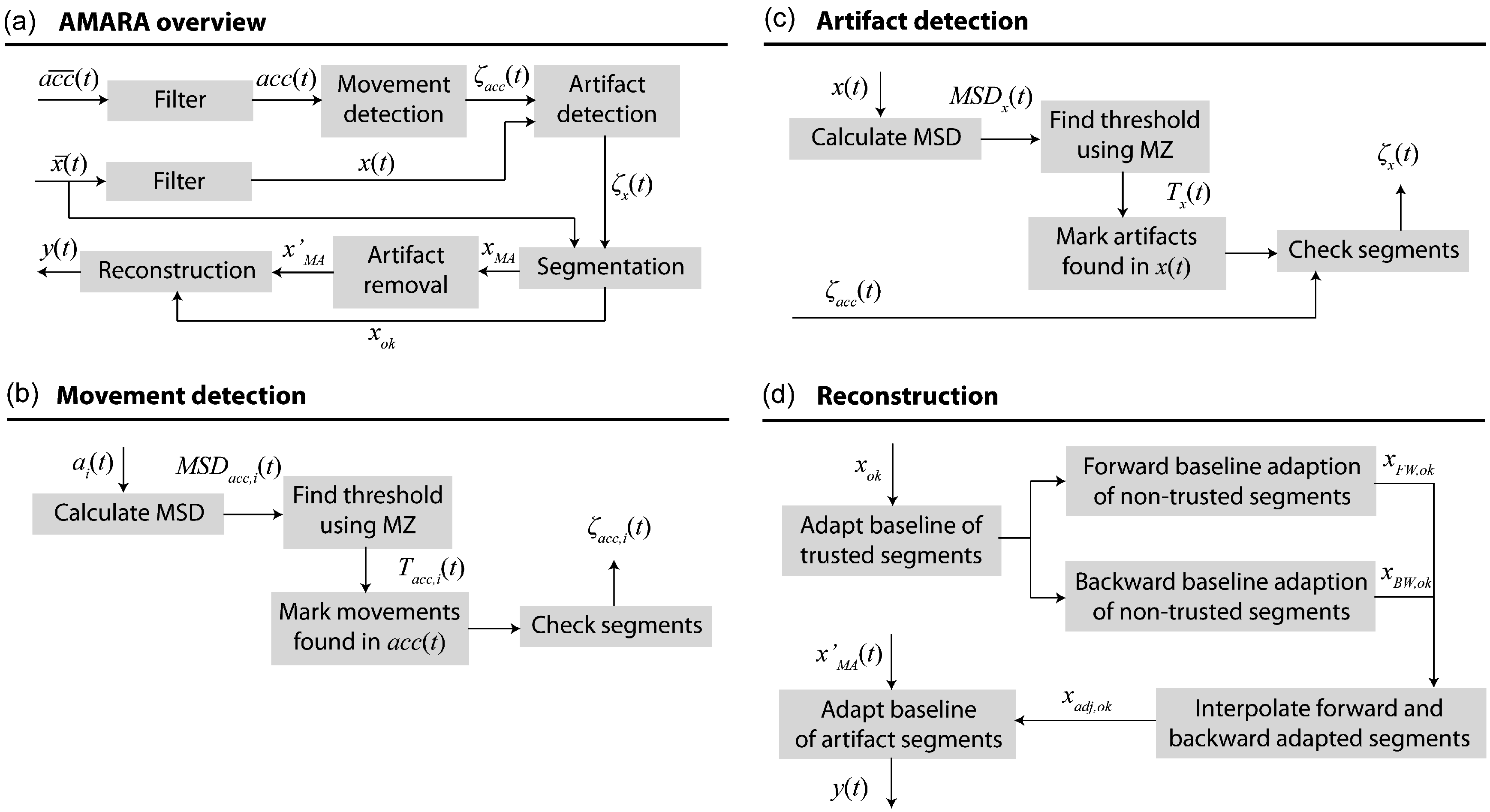
2.1. Algorithm

AMARA assumes that artifacts are always related to movements. Hence, it only accepts artifacts within movement periods of the subject, detected in the first step “movement detection”. The subsequent steps, i.e., artifact detection, segmentation, and artifact removal, were adapted from MARA [34] and were improved. The reconstruction of the signal was specifically developed for long-term recordings (8−10 h) including a criterion adapted from ABAMAR [63]. The algorithm was developed for application in sleep studies, thus the parameters given (summarized in Table 1) are optimized for such long-term recordings.

Table 1. List of parameters used in the AMARA algorithm. With the parameter values provided, the algorithm worked optimally in case of our recordings. However, the values depend on the specific characteristics of the input NIRS signals, e.g., number of MAs, frequency of occurrence of the MAs, amplitude of the MAs within the data, or the noise level. These parameters were chosen empirically to give the best result for the data sets comprising long-term NIRS measurements as reported by Metz et al. [21,22].

Parameter	Value	Description
q	2 s	Defines the MSD window length 2q + 1
wsize	15 min	Moving window length for the Zack triangle algorithm
wstep	5 min	Step size for the Zack triangle algorithm
Tarea	0.005	Noise criteria
Tareanorm	0.2	Normalized noise criteria
Lmin	2 s	Minimum allowed artifact size or gap between artifacts
“condition free”	no default	Defines the fixed segments for the reconstruction (no artifacts)
p	1 s	Window length for the FIR filter, Savitzky-Golay filter and MSD within the artifact removal procedure
fc,FIR	0.5 Hz	Cut-off frequency of the FIR filter within the artifact removal procedure

Table 1. List of parameters used in the AMARA algorithm. With the parameter values provided, the algorithm worked optimally in case of our recordings. However, the values depend on the specific characteristics of the input NIRS signals, e.g., number of MAs, frequency of occurrence of the MAs, amplitude of the MAs within the data, or the noise level. These parameters were chosen empirically to give the best result for the data sets comprising long-term NIRS measurements as reported by Metz et al. [21,22].

Parameter	Value	Description
q	2 s	Defines the MSD window length 2q + 1
wsize	15 min	Moving window length for the Zack triangle algorithm
wstep	5 min	Step size for the Zack triangle algorithm
Tarea	0.005	Noise criteria
Tareanorm	0.2	Normalized noise criteria
Lmin	2 s	Minimum allowed artifact size or gap between artifacts
“condition free”	no default	Defines the fixed segments for the reconstruction (no artifacts)
p	1 s	Window length for the FIR filter, Savitzky-Golay filter and MSD within the artifact removal procedure
fc,FIR	0.5 Hz	Cut-off frequency of the FIR filter within the artifact removal procedure

Figure 1. Flow charts of the whole algorithm (a) and detailed flow charts of specific steps (b−d). The algorithm detects movements and artifacts separately and only removes artifacts that coincide with a movement. The reconstruction is based on so-called trusted parts of the signal which are determined based on the acceleration signal. (a) AMARA flow chart. acc(t): time dependent acceleration signal with a x-, y- and z-component. $\overline{acc}\left(t\right)$: unfiltered acceleration signal. ξ_acc(t): output of the movement detection; every movement is marked by “1” at the corresponding sampling points. x(t): original signal (e.g., O₂Hb or HHb) containing MAs. $\overline{x}\left(t\right)$: unfiltered input signal. ξ_x(t): output of the artifact detection; every MA is marked by “1” at the corresponding sampling points. x_ok: container for only “ok” epochs (containing no MAs). x_MA: container for only artifact epochs (containing MAs). x’_MA: container, artifact epochs after MA removal, high frequency information is preserved. y(t): output signal of AMARA; of the same size as x(t), but with MAs removed and the reconstructed trend; (b) Movement detection flow chart. a_i(t): x-, y- or z-component of acc(t). ξ_acc,i(t) as in (a) but for a single component of acc(t). The final output vector is obtained by combining the three components (Equation (3), see text below). MSD: moving standard deviation. MZ: moving Zack triangle algorithm [64]. T_acc,i(t): vector containing the determined threshold for the acceleration signal; (c) Artifact detection flow chart for a signal x. The subscript x relates the variable to the signal x instead of the acceleration acc; (d) Reconstruction flow chart. x_FW,ok(t): “ok” epochs reconstructed in forward direction. x_BW,ok(t): “ok” epochs reconstructed in backward direction. x_adj,ok(t): “ok” epochs of forward and backward correction averaged.

Figure 1. Flow charts of the whole algorithm (a) and detailed flow charts of specific steps (b−d). The algorithm detects movements and artifacts separately and only removes artifacts that coincide with a movement. The reconstruction is based on so-called trusted parts of the signal which are determined based on the acceleration signal. (a) AMARA flow chart. acc(t): time dependent acceleration signal with a x-, y- and z-component. $\overline{acc}\left(t\right)$: unfiltered acceleration signal. ξ_acc(t): output of the movement detection; every movement is marked by “1” at the corresponding sampling points. x(t): original signal (e.g., O₂Hb or HHb) containing MAs. $\overline{x}\left(t\right)$: unfiltered input signal. ξ_x(t): output of the artifact detection; every MA is marked by “1” at the corresponding sampling points. x_ok: container for only “ok” epochs (containing no MAs). x_MA: container for only artifact epochs (containing MAs). x’_MA: container, artifact epochs after MA removal, high frequency information is preserved. y(t): output signal of AMARA; of the same size as x(t), but with MAs removed and the reconstructed trend; (b) Movement detection flow chart. a_i(t): x-, y- or z-component of acc(t). ξ_acc,i(t) as in (a) but for a single component of acc(t). The final output vector is obtained by combining the three components (Equation (3), see text below). MSD: moving standard deviation. MZ: moving Zack triangle algorithm [64]. T_acc,i(t): vector containing the determined threshold for the acceleration signal; (c) Artifact detection flow chart for a signal x. The subscript x relates the variable to the signal x instead of the acceleration acc; (d) Reconstruction flow chart. x_FW,ok(t): “ok” epochs reconstructed in forward direction. x_BW,ok(t): “ok” epochs reconstructed in backward direction. x_adj,ok(t): “ok” epochs of forward and backward correction averaged.

In Figure 1a the signal processing steps are shown as a flow chart. Note that the “Filter” blocks should equalize the acceleration signal acc and the hemoglobin signal x in terms of the noise levels (i.e., standard deviation of the signals should be comparable). The same automated threshold detection was applied to both signals and the detection criteria depended on the noise level. The algorithm was implemented in Matlab^® (Version 2008b, The MathWorks^®, Natick, MA, USA).

2.1.1. Movement Detection

Figure 1b depicts the four necessary steps to detect movements in the acceleration signal acc(t), which is the vector of the x-, y- and z-acceleration components (i.e., acc(t) = [a_x(t), a_y(t), a_z(t)]). The final output of the movement detection is a vector ξ_acc(t) which contains “1” whenever a movement was found and zero otherwise. This vector is calculated by the following steps:

Step 1: First, the moving standard deviation (MSD) of acc(t) is calculated:

$$MS{D}_{acc,i}\left(t\right)={\left[\frac{1}{2q+1}{\displaystyle \sum }_{j=-q}^q{\left(a_i\left(t+j\right)-\frac{1}{2q+1}{\displaystyle \sum }_{j=-q}^q{a}_i\left(t+j\right)\right)}^2\right]}^{\frac{1}{2}}$$

(1)

where the MSD window length is given by 2q + 1 samples and i represents the components x, y, or z. The value of q used here is twice the number of samples per second of the signal, i.e., representing two seconds for the NIRS data used in the present study. Thus, q = 2 s × f_s (i.e., two seconds times the sampling frequency f_s in Hz = 2 s of data), whereas f_s has to be an integer.

Step 2: The threshold T_acc(t) for the detection of movements is determined automatically using the moving Zack triangle algorithm [64]. This method finds T_acc(t) based on the quantile distribution D (equal to the inverse cumulative distribution) of the data within a certain window of length w_size (see Figure 2). A line L is drawn from the smallest to the largest quantile within D (Figure 2e,f) and the normal (black line marked with a 90° angle in Figure 2f) to L is moved to find the maximum length between L and D [64]. The threshold T_acc corresponds to the y-value of the intersection of the normal with D. Now a threshold is defined for the first w_size seconds of MSD_acc,i(t). To find the threshold T_acc(t) for the rest of the signal, a window of the length w_size is moved forward by the step size w_step and the algorithm is applied again. The values used for w_size and w_step were 15 × 60 s × f_s and 5 × 60 s × f_s, respectively. This represents 15 and 5 min of data. Since the step size w_step is smaller than the window size w_size, the calculated thresholds overlap. To avoid overlapping of the thresholds, the threshold is only set for the center w_step data points within the window of size w_size. Hence, T_acc[t − w_step/2 ,…, t + w_step/2] = MZA([MSD_acc,i[t − w_size/2 ,…, t + w_size/2]). MZA represents the application of the moving Zack triangle algorithm and t is the time point in the center of the window of size w_size.

The Zack triangle algorithm is not able to distinguish a noisy, but valid, biological signal (= “Noise” in Figure 2) from an artifact. Hence, two conditions had to be applied to identify noise afterwards: the area between L and D, and the normalized area between L and D (Figure 2e,f). The normalized area was obtained from the normalized quantile distribution, defined as D/max(D). If one of these values was smaller than the thresholds T_area (typically 0.005) or T_areanorm (typically 0.2), respectively, the data in the window were considered to be noise and the threshold T_acc was set to infinity. For example, if normally distributed noise dominates the signal, the absolute and normalized area between L and D approach zero. If there is a (small) peak within normally distributed noise, the normalized threshold will be large, but the absolute area will be small. In case of non-normally distributed noise or when different noise levels are present in the data, the absolute area might be large, but the normalized area will still be small. The T_areanorm condition corresponds to a peak that exceeds approximately three times the SD of the examined part of the MSD (of the length w_size).

Figure 2. Example of noise detection (left column: a,c,e) and artifact detection (right column: b,d,f) in [O₂Hb] data (sampling rate: 35 Hz). Top row (a,b): original signal. Middle row (c,d): moving standard deviation (MSD) of the input signal. Bottom row: quantiles from 0 to 1 in steps of 0.01 of the corresponding MSD values. “A” is the area between the quantile distribution (D) and the straight line (L) connecting the first and the last quantile. A_norm is A normalized, i.e., the distribution was divided by its maximum value. On the bottom right (f), the Zack triangle method is displayed which leads to a threshold of approximately 0.4 μM. For a detailed description, please refer to the text. Small inserts in the top (b) and middle right (d) panel depict the artifact on a magnified time scale (~14.3 s).

Figure 2. Example of noise detection (left column: a,c,e) and artifact detection (right column: b,d,f) in [O₂Hb] data (sampling rate: 35 Hz). Top row (a,b): original signal. Middle row (c,d): moving standard deviation (MSD) of the input signal. Bottom row: quantiles from 0 to 1 in steps of 0.01 of the corresponding MSD values. “A” is the area between the quantile distribution (D) and the straight line (L) connecting the first and the last quantile. A_norm is A normalized, i.e., the distribution was divided by its maximum value. On the bottom right (f), the Zack triangle method is displayed which leads to a threshold of approximately 0.4 μM. For a detailed description, please refer to the text. Small inserts in the top (b) and middle right (d) panel depict the artifact on a magnified time scale (~14.3 s).

Step 3: For each sample point (t) a value of “0” or “1” is assigned to a vector ξ_acc(t), depending on the SD and the thresholds. To obtain only one vector from the three acceleration components, the individual ξ_acc,i(t) are combined by a logic OR operation (Equation (3)):

$${\mathsf{\xi }}_{\text{acc},\text{i}}\left(\text{t}\right)=\{\begin{array}{c}1, \text{if} {\text{MSD}}_{\text{acc},\text{i}}\left(t\right)>{\text{T}}_{\text{acc},\text{i}}\left(t\right)\\ 0, {\text{if MSD}}_{\text{acc},\text{i}}\left(\text{t}\right)\le {\text{T}}_{\text{acc},\text{i}}\left(t\right)\end{array},\text{ for i}=\text{x},\text{y},\text{z}$$

(2)

$${\mathsf{\xi }}_{\text{acc}}\left(\text{t}\right)={\text{ ξ}}_{\text{acc},\text{x}}\left(\text{t}\right)\bigvee {\text{ ξ}}_{\text{acc},\text{y}}\left(\text{t}\right)\bigvee {\text{ ξ}}_{\text{acc},\text{z}}\left(\text{t}\right)$$

(3)

Step 4: If the length of a movement segment is shorter than L_min, ξ_acc is set to “0” again at the corresponding time points. Correspondingly, if the gap between two movement segments is shorter than L_min, this gap is also set to be a movement. This reduces false positive detections due to the Zack triangle algorithm, which often sets the threshold very conservatively, i.e., slightly higher than the noise level. It is statistically possible that the MSD of the noise also exceeds the threshold but then only for a very short period. This behavior can be controlled by adjusting L_min. The value of L_min used was 2 s × f_s. The final output of the movement detection process is the vector ξ_acc(t) which contains values of “1” at samples assigned to be a MA.

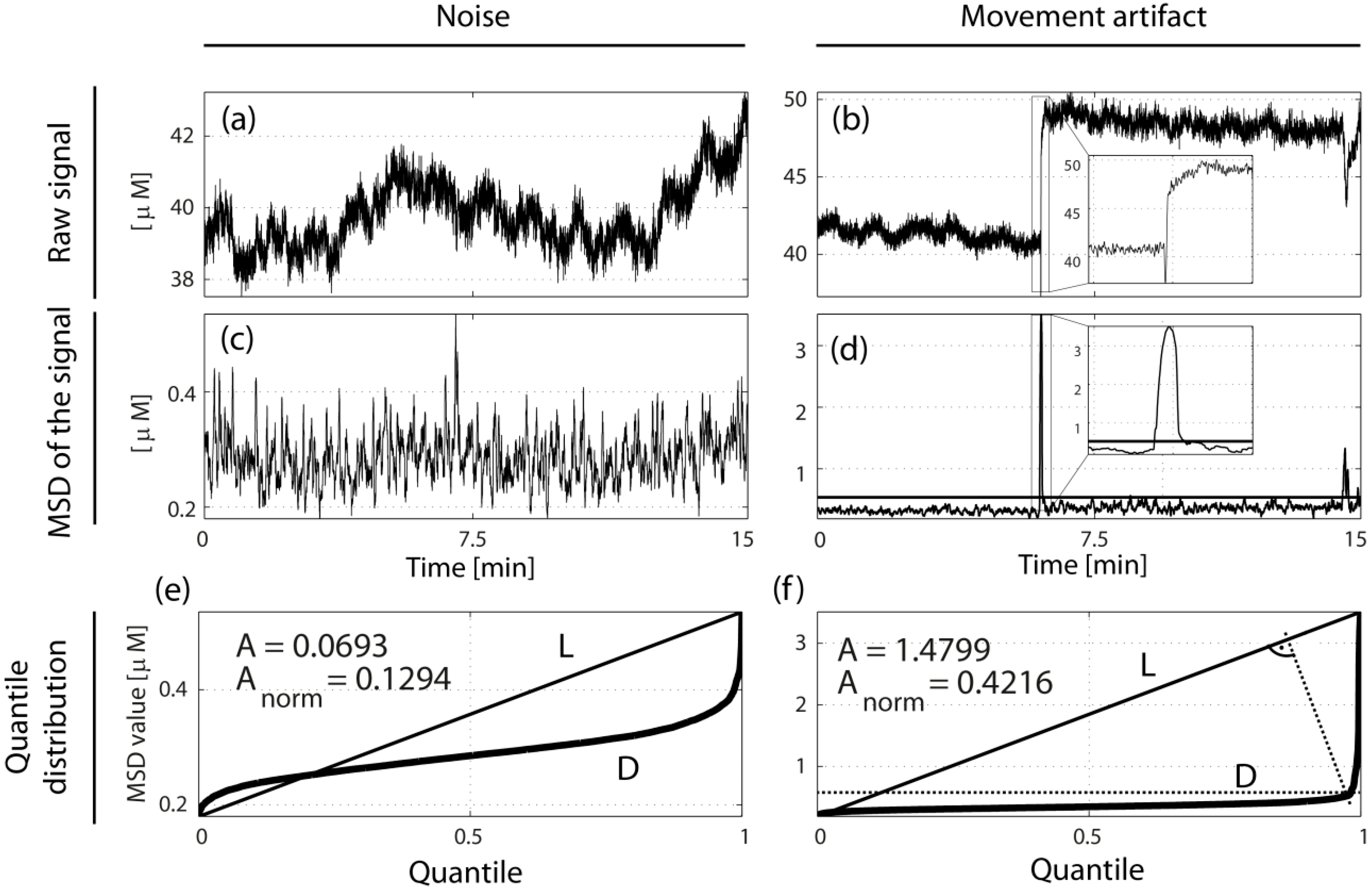
2.1.2. Artifact Detection

In Figure 1c, the basic flow chart for the detection of artifacts within the signal x(t) is illustrated. These four steps are similar to the movement detection, as is the output vector ξ_x(t), which contains “1” at time points found to be an artifact and “0” otherwise.

Step 1: MSD_x(t) of the signal x(t) is calculated as described in Step 1 of Section 2.1.1 Movement detection.

Step 2: The threshold T_x(t) for the artifact detection is obtained automatically using the moving Zack triangle algorithm, as in Step 2 of Section 2.1.1 Movement detection.

Step 3: All values of the signal MSD_x(t) greater than T_x(t) are marked as “1”, as in Step 3 of Section 2.1.1 Movement detection:

$${\xi }_x\left(t\right)=\{\begin{array}{c}1 \text{if} MS{D}_x\left(t\right)>T_x\left(t\right)\\ 0 \text{if }MS{D}_x\left(t\right)\le T_x\left(t\right)\end{array}$$

(4)

Step 4: Finally the information from the accelerometer ξ_acc(t) is used to verify that the artifact is caused by a movement. For each artifact, the corresponding movement containing vector ξ_acc(t) is checked. If this contains no movement (thus only “0”) for the time points of interest, ξ_x(t) will be set to “0” for the corresponding time points. Mathematically, this corresponds to a logic AND operation:

$${\xi }_x\left(t\right)= {\xi }_{acc}\left(t\right) \wedge {\xi }_x\left(t\right)$$

(5)

Furthermore, the algorithm rejects all artifacts shorter than L_min. This was done for the same reason as in Step 4 of Section 2.1.1 Movement detection.

2.1.3. Segmentation

The data were segmented as in the MARA algorithm. The segmentation vector contains N entries. There are two kinds of segments: segments containing MAs (“MA” segments) and segments containing no artifacts (“ok” segments). The beginning and end of each segment is identified based on the change of values in the vector ξ_x(t). A change from “0” to “1” determines the beginning of an artifact (and end of an “ok” segment) and a change from “1” to “0” its end (and start of a new “ok” segment). The segmentation container t_Seg,k contains the time points ${\stackrel{\rightharpoonup }{t}}_k$ (vector addressing all time points for the segment) for each segment k and can be expressed as:

$$\begin{array}{cc}{t}_{Seg,k}=\left\{{\stackrel{\rightharpoonup }{t}}_{ok,1},{\stackrel{\rightharpoonup }{t}}_{MA,2},{\stackrel{\rightharpoonup }{t}}_{ok,3},{\stackrel{\rightharpoonup }{t}}_{MA,4},\cdots ,{\stackrel{\rightharpoonup }{t}}_{MA,N-1},{\stackrel{\rightharpoonup }{t}}_{ok,N}\right\},& \text{for }k=\left\{1,\dots ,N\right\}\end{array}$$

(6)

$$\mathit{a}\mathit{c}{\mathit{c}}_{\mathit{k}}= \mathit{a}\mathit{c}\mathit{c}\left(t_{Seg,k}\right),\text{ for }k=\left\{1,\dots ,N\right\}$$

(7)

$$x_k= x\left(t_{Seg,k}\right), \text{for }k=\left\{1,\dots ,N\right\}$$

(8)

Furthermore, we define the MA segments to be

$$\mathit{a}\mathit{c}{\mathit{c}}_{\mathit{M}\mathit{A},\mathit{m}}= \mathit{a}\mathit{c}\mathit{c}\left(t_{Seg,2m}\right),\text{ for} m=\left\{1,\dots ,\left(N-1\right)/2\right\}$$

(9)

$$x_{MA,m}=x\left(t_{Seg,2m}\right),\text{ for }m=\left\{1,\dots ,\left(N-1\right)/2\right\}$$

(10)

The variable m is another index variable needed to address all even segments. The “ok” segments are defined in a similar way for the odd entries in acc and x. A classification condition C_k is defined based on the x-, y- and z-components of the acceleration signal acc(t):

$$C_k=\{\begin{array}{c}1, \text{if} \mathit{a}\mathit{c}\mathit{c}\left(t_{Seg,k}\right)\in \left\{\text{condition free}\right\} \\ 0, \text{if} \mathit{a}\mathit{c}\mathit{c}\left(t_{Seg,k}\right)\in \left\{\text{condition not free}\right\}\end{array} ,\text{ for }k=\left\{1,\dots ,N\right\}$$

(11)

whereas C_MA,m and C_Ok,n (n = {1,…,(N−1)/2+1}) can be defined in a similar way as above. The terms “condition free” and “condition not free” refer to ranges for the acceleration values of the x-, y- and z-axes. This classification gives trustworthy baseline regions. For example, during sleep, baseline shifts of the signal were observed whenever the subject lied on the NIRS sensor (pressure on the sensor: “condition not free”) compared to when the sensor is free (not jammed between bed and subject: “condition free”). Thresholds for the determination of the two states were determined after examining the entire dataset manually. Video recordings were inspected to determine “not free” positions and to derive the corresponding acceleration thresholds. Since the sensor was always in a specific position during the position “condition not free”, simple thresholds could be applied to the acceleration signals to determine the “condition not free” position. Furthermore, this information was used for the reconstruction of the signal.

2.1.4. Artifact Removal

The artifact removal is similar to MARA but was extended in order to preserve physiological information. MARA includes the interpolation of the MA segment with a spline function and the subtraction of the interpolated segment from the original segment to preserve the high frequency information of the signal. In the current implementation we used an nth-order Savitzky-Golay filter [65] since this allowed to model sharp rises in the signal (i.e., an artifact) while being computationally inexpensive. However, during an “ok” period of the signal, it will also exclude true physiological information. To overcome this caveat, the Savitzky-Golay filtered signal x_k,SG was weighted according to MSD_k, the MSD of x_k, but with the window length p (substitute q with p in Equation (1)) and thus different from MSD_x. MSD_k was further normalized to a range [0, 1] by MSD_k/max(MSD_k). x_k,SG was complemented with a finite infinite response (FIR) low-pass filtered signal x_k,FIR. x_k,FIR is weighted complementary with 1 − (MSD_k/max(MSD_k)). The complete signal is recovered by adding x_k,FIR and the x_k,SG. Put simply, the Savitzky-Golay filter was applied to abrupt signal changes (i.e., the artifacts) and the FIR filter during the stable parts of the signal. The window lengths (parameter p) of the FIR filter, the Savitzky-Golay and the MSD were set to p = f_s × 1 s samples (Table 1). Furthermore, the order of the Savitzky-Golay filter was set to 3 and the low-pass cutoff frequency f_c,FIR of the FIR filter to 0.5 Hz if the heart beat (approximately 1 Hz) was of interest (preservation of the desired physiological information). This filtered signal was subtracted from the original signal and the following vector was obtained:

$$x{\prime }_{MA,m}=AR\left\{x_{MA,m}\right\},\text{ for }m=\left\{1,\dots ,\left(N-1\right)/2\right\}$$

(12)

The dash and the operator AR (artefact removal) indicate that the procedure outlined above was applied. The mean of the high-pass filtered segment is zero and will be adapted to the “ok” segments of baseline during the following reconstruction.

2.1.5. Reconstruction

In contrast to the reconstruction performed by MARA, where the segments are baseline corrected one by one, AMARA reconstruction is based on “ok” segments only (as with ABAMAR) and AMARA reconstructs the signal by including additional information from the acceleration sensor. MARA includes the (artifact removed) MA segments in the reconstruction. AMARA assumes that the length of the MA is small compared to the adjacent “ok” segments. The signal changes are expected to be within the magnitude of the standard deviations of the signal in adjacent segments. Based on the value of C_k, AMARA assumes that the segments labeled with “condition free” (C_k = 1) represent “trustworthy” values. Those labeled as “condition not free” (C_k = 0) are not trusted and the corresponding signal may deviate from the original baseline. The baseline was defined as the mean of last or first part (of length L_base, e.g., 20 s) of a segment. Between trustworthy segments (“condition free”) a baseline shift may also be present. In such a case, the longest of all connected trustworthy segments will be used and the others will be adjusted to this level. The reconstruction comprises the following steps (see Figure 1d):

Step 1: Find and adjust all the baselines of connected trustworthy segments. “Connected” is defined to be a group of segments with C_ok,k = 1, which are not separated by any other “ok” segment with C_ok,k = 0. MA segments are disregarded at this point. For each group, starting with the longest segment m, all following segments (m + 1, m + 2, etc.) are adjusted to the former segment’s baseline. Similarly the baseline of the previous segments (m − 1, m − 2, etc.) are adjusted. The baseline of the earlier segment (in time) is the last part of length L_base (e.g., 20 s) and has the average ${\overline{x}}_{ok,m}$ and the SD σ_ok,m. The later segment’s baseline is defined to be the first part of length L_base with the average ${\overline{x}}_{ok,m+1}$ and the SD σ_ok,m+1. The later segment is only “adjusted” if the difference between the baselines is larger than 2.6 times the SD, a criterion adapted from ABAMAR. The factor 2.6 corresponds to the 99^th percentile of normally distributed data.

$$x_{adj,ok,m+1}=\{\begin{array}{ccc}{x}_{ok,m+1}-\left({\overline{x}}_{ok,m+1}-{\overline{x}}_{adj,ok,m}\right),& \text{if}& \left|{\overline{x}}_{ok,m+1}-{\overline{x}}_{ok,m}\right|\ge 2.6{\sigma }_{ok,m}\\ x_{ok,m+1}-\left({\overline{x}}_{ok,m}-{\overline{x}}_{adj,ok,m}\right),& \text{if}& \left|{\overline{x}}_{ok,m+1}-{\overline{x}}_{ok,m}\right|<2.6 {\sigma }_{ok,m}\end{array}$$

(13)

The previous segments’ baseline is adjusted similarly to the later segments’ baseline:

$$x_{adj,ok,m-1}=\{\begin{array}{ccc}{x}_{ok,m-1}-\left({\overline{x}}_{ok,m-1}-{\overline{x}}_{adj,ok,m}\right),& \text{if}& \left|{\overline{x}}_{ok,m-1}-{\overline{x}}_{ok,m}\right|\ge 2.6{\sigma }_{ok,m}\\ x_{ok,m-1}-\left({\overline{x}}_{ok,m}-{\overline{x}}_{adj,ok,m}\right),& \text{if}& \left|{\overline{x}}_{ok,m-1}-{\overline{x}}_{ok,m}\right|<2.6{\sigma }_{ok,m}\end{array}$$

(14)

Step 2: Adjust the baseline of all not trusted (“condition not free”) segments in a forward loop. Starting with the first segment with C_k = 0 after the first trustworthy segment, the baseline of the segments with C_k = 0 is adapted to the former segments baseline. The baseline is shifted as in Equation (13). The resulting segments are saved in the vector x_FW,ok,m.

Step 3: Adjust the baseline of all not trusted (“condition not free”) segments in a backward loop. Starting at the first segment with C_k = 0 before the last trustworthy segment, the baseline of the segments with C_k = 0 are adapted to the later segments’ baseline. The baseline is shifted similarly as in Equation (14). The resulting segments are saved in the vector x_BW,ok,m.

Step 4: Interpolate the forward and backward adjusted baselines of all not trusted (“condition not free”) segments. For every segment with C_k = 0 between two trustworthy segments the final reconstruction is calculated as:

$$\begin{array}{ccc}{x}_{adj,ok,m+j}=\frac{L\prime -j+1}{L\prime +1}{x}_{FW,ok,m+j}+\frac{j}{L\prime +1}{x}_{BW,ok,m+j} ,& \text{if}& C_{m+j}=0\end{array}$$

(15)

Here L′ is the number of segments between the two closest trustworthy segments and j is relative position of the segment within this group. Hereby j = 1 would be assigned to the temporally earliest segment and j = L′ is assigned to the temporally latest segment. All not trustworthy segments before the first trustworthy segment are equal to the backward adjusted segments x_BW,ok,m. At the back of the signal, all not trusted segments after the last trustworthy segment are equal to the forward adjusted segments x_FW,ok,m.

Step 5: Adjust the baseline of all MA segments. The baseline of the artifact segments is adapted to the “ok” segments:

$$\begin{array}{cc}{x}_{adj,MA,m}=x{\prime }_{MA,m}+\left({\overline{x}}_{adj,ok,m}+{\overline{x}}_{adj,ok,m+1}\right)/2,& \text{for }m=\left\{1,\dots ,N/2\right\}\end{array}$$

(16)

As described in Step 1 of Section 2.1.5 Reconstruction, ${\overline{x}}_{adj,ok,m}$ is the average value of the last L_base seconds of the previous “ok” segment and ${\overline{x}}_{adj,ok,m+1}$ is the average value of the first L_base seconds of the following “ok” segment.

After this step, the reconstructed signal y(t) is given by:

$$y\left(t\right)=\left\{x_{adj,ok,1},x_{adj,MA,1},\cdots ,x_{adj,ok,\left(N-1\right)/2},x_{adj,MA,\left(N-1\right)/2},x_{adj,ok,\left(N+1\right)/2}\right\}$$

(17)

2.2. Validation

2.2.1. Measurements

We used overnight NIRS measurements of cerebral (prefrontal) [O₂Hb] and [HHb] to validate the algorithm. Twelve healthy adolescent males (age 10–16 years) slept on two separate nights in the sleep laboratory of the University Children’s Hospital Zurich, Switzerland. The mean sleep time was 8.5 h. The detailed protocol is described in Metz et al. [21,22]. The study was approved by the ethical committee of the Canton of Zurich and informed consent was signed by the legal representatives of the adolescents.

2.2.2. NIRS Instrumentation

Measurements of cerebral hemodynamics and oxygenation were performed by the OxyPrem NIRS device. It is a three wavelength (760, 805 and 870 nm) continuous wave NIR spectroscope developed in-house which is electronically similar to a previously described device [66]. The NIRS optode employs four sources and two detectors at two different source-detector separations (1.5 and 2.5 cm). Detectors and sources are connected by a flexible printed circuit board, i.e., relative movements were possible to some extent. The data were recorded at a sampling frequency of 35 Hz. [O₂Hb] and [HHb] were calculated by the self-calibrating algorithm [44] for two different regions including two sources and two detectors each. A schematic drawing of the sensor can be found in Figure 6a of reference [2]. The self-calibrating algorithm cancels long-term drifts, e.g., drift from light sources [44]. OxyPrem is embedded into soft medical grade black-colored silicone to ensure comfort of the subjects. It additionally featured an accelerometer (ADXL330, Analog Devices, Norwood, MA, USA; sensitivity: 0.3 V/g, resolution 8 bit, i.e., 26 analog to digital converter units per g) to monitor the subject’s movements. The accelerometer was soldered directly next to one of the two detectors within the silicon mold. The accelerometer data were sampled synchronically with the NIRS data at 35 Hz. The NIRS optode was placed at the subject’s left forehead, approximately above the left prefrontal cortex.

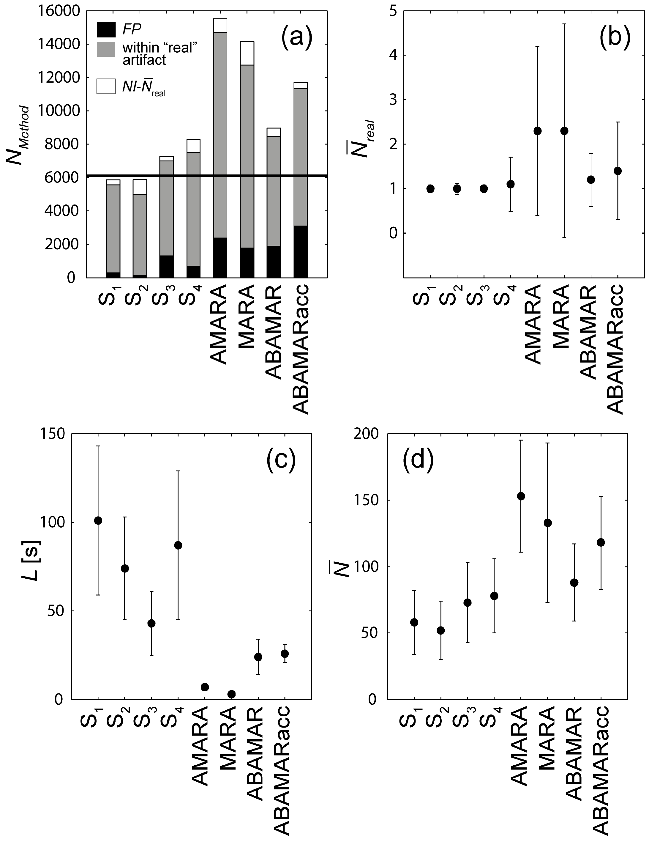
2.2.3. Validation of AMARA against Human Scorers, MARA and ABAMAR

The new algorithm (AMARA) was validated against (i) manual artifact scoring by experts with experience in NIRS data processing; (ii) MARA; and (iii) ABAMAR. Four expert human scorers (S₁–S₄) identified manually the artifacts in the 24 recordings. These experts had a minimum of two years of experience in post-processing of large NIRS data sets, however with different applications. For MARA, the same MSD parameters were used as for AMARA. ABAMAR was implemented adopting the parameters given in [63] except for the motion detection threshold, which was set to 0.2–0.55 g/s in order to be better adapted to our measured data (g: earth’s gravity). AMARA was applied to [O₂Hb] and [HHb] time series. [O₂Hb] and [HHb] time series of the long light path (source-detector separation: 2.5 cm) was used.

The [O₂Hb] and [HHb] time series were segmented into 30 min time periods and presented to the scorer (S₁ to S₄) one after the other. The subsequent presentation of 30 min time periods helped to increase the accuracy of the scoring. In addition to the NIRS data, the corresponding acceleration signals for the x-, y- and z-axis were presented simultaneously to the scorer (plot not shown). Four signals (2 × HHb and 2 × O₂Hb) were evaluated in each night, because the sensor measured two brain regions. This led to a total of 96 signals with a mean duration of 8.5 h. A binary artifact signal was obtained from each scorer containing “1” for every time point scored as an artifact. An artifact was considered as a “real” artifact when at least three human scorers marked it as artifact. The following measures were calculated to compare the different algorithms: (i) the total number of artifacts (N_Method) identified in all recordings identified by each method; (ii) the total number of “real” artifacts (N_real); (iii) the average number of artifacts per signal calculated as the total amount of artefacts divided by the 24 measurements and the four signals per measurement ($\overline{N}$ = N_Method/24/4); (iv) the mean length of an artifact (L); (v) the number of not identified “real” artifacts (NI); (vi) the sensitivity of the method S = (N_real – NI)/N_real; (vi) the mean number of artifacts within a “real” artifact (${\overline{N}}_{real}$), and (vii) the number of false positives (FP), defined as the number of detected artifacts not occurring within a “real” artifact. To compare AMARA with MARA, all artifacts found by MARA were set to “true” and FP, NI, S and ${\overline{N}}_{real}$ were compared. To compare specifically the movement detection between AMARA and ABAMAR, only the ABAMAR artifacts were set to “true” and again FP, NI, S and ${\overline{N}}_{real}$ were compared. In addition to the artifacts found by AMARA, artifacts found only by the movement detection of AMARA were also taken into account (denoted by AMARAacc in Table 2 and Table 3).

Table 2. Performance of artifact detection of AMARA, MARA, ABAMAR and the human scorers S₁ – S₄. In total, each scorer analyzed 96 signals. N_Method: number of total artifacts found. $\overline{N}$: average number of artifacts scored per signal ± SD. L: average length of the artifacts in s ± SD. NI: not identified artifacts; as percentage of “real” artifacts N_real in parenthesis. S: sensitivity S = (NI – N_real)/N_real. ${\overline{N}}_{real}$: average number of artifacts detected within a “real” artifact ± SD. “Real” artifacts are those identified by at least 3 of the 4 human scorers. The total number of “real” artifacts was 6228. FP: number of false positive detections; as percentage of the total number N_Method of artifacts in parenthesis.

	S1	S2	S3	S4	AMARA	MARA	ABAMAR	AMARAacc
NMethod	5553	5011	6998	7526	14,695	12,732	8478	11,334
$\overline{N}$	58 ± 24	52 ± 22	73 ± 30	78 ± 28	153 ± 42	133 ± 60	88 ± 29	118 ± 35
L [s]	101 ± 42	74 ± 29	43 ± 18	87 ± 42	7 ± 2	3 ± 1	24 ± 10	26 ± 5
NI	306 (4.9%)	866 (13.9%)	269 (4.3%)	768 (12.3%)	823 (13.2%)	1427 (22.9%)	487 (7.8%)	362 (5.8%)
S	95.1%	86.1%	95.7%	87.7%	86.8%	77.1%	92.2%	94.2%
${\overline{N}}_{real}$	1 ± 0.08	1 ± 0.12	1 ± 0.08	1.1 ± 0.61	2.3 ± 1.9	2.3 ± 2.4	1.2 ± 0.6	1.4 ± 1.1
FP	280 (5.0%)	144 (2.9%)	1301 (18.6%)	674 (9.0%)	2374 (16.2%)	1779 (14.0%)	1889 (22.3%)	3088 (27.2%)

Table 2. Performance of artifact detection of AMARA, MARA, ABAMAR and the human scorers S₁ – S₄. In total, each scorer analyzed 96 signals. N_Method: number of total artifacts found. $\overline{N}$: average number of artifacts scored per signal ± SD. L: average length of the artifacts in s ± SD. NI: not identified artifacts; as percentage of “real” artifacts N_real in parenthesis. S: sensitivity S = (NI – N_real)/N_real. ${\overline{N}}_{real}$: average number of artifacts detected within a “real” artifact ± SD. “Real” artifacts are those identified by at least 3 of the 4 human scorers. The total number of “real” artifacts was 6228. FP: number of false positive detections; as percentage of the total number N_Method of artifacts in parenthesis.

	S1	S2	S3	S4	AMARA	MARA	ABAMAR	AMARAacc
NMethod	5553	5011	6998	7526	14,695	12,732	8478	11,334
$\overline{N}$	58 ± 24	52 ± 22	73 ± 30	78 ± 28	153 ± 42	133 ± 60	88 ± 29	118 ± 35
L [s]	101 ± 42	74 ± 29	43 ± 18	87 ± 42	7 ± 2	3 ± 1	24 ± 10	26 ± 5
NI	306 (4.9%)	866 (13.9%)	269 (4.3%)	768 (12.3%)	823 (13.2%)	1427 (22.9%)	487 (7.8%)	362 (5.8%)
S	95.1%	86.1%	95.7%	87.7%	86.8%	77.1%	92.2%	94.2%
${\overline{N}}_{real}$	1 ± 0.08	1 ± 0.12	1 ± 0.08	1.1 ± 0.61	2.3 ± 1.9	2.3 ± 2.4	1.2 ± 0.6	1.4 ± 1.1
FP	280 (5.0%)	144 (2.9%)	1301 (18.6%)	674 (9.0%)	2374 (16.2%)	1779 (14.0%)	1889 (22.3%)	3088 (27.2%)

Table 3. Left part: Detection performance comparing artifacts identified by AMARA, AMARAacc and ABAMAR with MARA. The MARA artifacts (12,732 in total) were considered as the true ones, i.e., MARA was the reference for comparison with the other algorithms. Thus, MARA has a sensitivity of 100%, no false positives and no missed ones. Right part: Comparison of the movement detection process; the ABAMAR (where the artifact detection only relies on the acceleration signals) artifacts (8478 total) have been set as true. Please refer to Table 2 for the description of the variables. AMARAacc: Movement detection part (Section 2.1.1) of the AMARA algorithm. Thus, only artifacts identified with accelerometer data were considered as artifacts.

	Artifacts Identified				Movements Detected
	MARA	AMARA	AMARAacc	ABAMAR	ABAMAR	AMARAacc
NI	0 (0%)	2739 (21.5%)	2271 (17.8%)	2410 (18.9%)	0 (0%)	686 (8.1%)
S	100%	78.5%	82.2%	81.1%	100%	91.9%
${\overline{N}}_{real}$	1 ± 0.00	1 ± 0.07	1 ± 0.05	1 ± 0.00	1 ± 0.00	1.2 ± 0.78
FP	0 (0%)	6793 (46.2%)	5116 (45.1%)	3195 (37.7%)	0 (0%)	1969 (17.4%)

Table 3. Left part: Detection performance comparing artifacts identified by AMARA, AMARAacc and ABAMAR with MARA. The MARA artifacts (12,732 in total) were considered as the true ones, i.e., MARA was the reference for comparison with the other algorithms. Thus, MARA has a sensitivity of 100%, no false positives and no missed ones. Right part: Comparison of the movement detection process; the ABAMAR (where the artifact detection only relies on the acceleration signals) artifacts (8478 total) have been set as true. Please refer to Table 2 for the description of the variables. AMARAacc: Movement detection part (Section 2.1.1) of the AMARA algorithm. Thus, only artifacts identified with accelerometer data were considered as artifacts.

	Artifacts Identified				Movements Detected
	MARA	AMARA	AMARAacc	ABAMAR	ABAMAR	AMARAacc
NI	0 (0%)	2739 (21.5%)	2271 (17.8%)	2410 (18.9%)	0 (0%)	686 (8.1%)
S	100%	78.5%	82.2%	81.1%	100%	91.9%
${\overline{N}}_{real}$	1 ± 0.00	1 ± 0.07	1 ± 0.05	1 ± 0.00	1 ± 0.00	1.2 ± 0.78
FP	0 (0%)	6793 (46.2%)	5116 (45.1%)	3195 (37.7%)	0 (0%)	1969 (17.4%)

3. Results

3.1. Validation against the Human Scorers

In total, 6228 “real” artifacts were identified (i.e., at least three out of four human scorers agreed). An overview of the validation results can be found in Table 2 and Figure 3. The sensitivity to “real” artifacts of AMARA was S = 86.8%. The human scorers reached a sensitivity of S = 86%−96%, ABAMAR 92.2% and MARA 77.1%. AMARA had a higher sensitivity when only the movement detection was taken into account (taking place before the MA detection; S = 94.2%, AMARAacc in Table 2). This was higher than ABAMAR’s sensitivity, which relies on its detection only on the accelerometer signal and is directly comparable. It was also close to the sensitivity of the human scorers S₁ and S₃. This means that AMARA’s sensitivity is reduced due to rejection of MAs within identified movement epochs. One explanation might be that small (in terms of amplitude) artifacts close to large artifacts were not detected. The large artifacts possibly elevated the detection threshold above the amplitude of small artifacts. Subtle movements accounted most likely for the remainder of the undetected artifacts of AMARA (461 of 823, NI = 44%). Slow movements below the detection level may have caused this problem; it may also have been possible that some artifacts were not related to movements.

Figure 3. Summary of the validation results. (a) Number of total artifacts (N_Method), subdivided into false positives (FP, black) and true positives within 'real' artifacts (grey) and not identified (NI, white). The total number of artifacts found by each algorithm/human scorer is represented by the sum of 'within "real" artifact' + FP. The horizontal line represents N_real = 6228; (b) The mean number of artifacts detected within one “real” artifact (${\overline{N}}_{real}$); (c) The mean length (L) of identified artifact segments; (d) The average number ($\overline{N}$) of artifacts identified per recorded signal ([O₂Hb] or [HHb]). S₁–S₄: human scorers no. 1–4. Error bars always represent the standard deviation.

Figure 3. Summary of the validation results. (a) Number of total artifacts (N_Method), subdivided into false positives (FP, black) and true positives within 'real' artifacts (grey) and not identified (NI, white). The total number of artifacts found by each algorithm/human scorer is represented by the sum of 'within "real" artifact' + FP. The horizontal line represents N_real = 6228; (b) The mean number of artifacts detected within one “real” artifact (${\overline{N}}_{real}$); (c) The mean length (L) of identified artifact segments; (d) The average number ($\overline{N}$) of artifacts identified per recorded signal ([O₂Hb] or [HHb]). S₁–S₄: human scorers no. 1–4. Error bars always represent the standard deviation.

Figure 4. (a) Comparison of the performance in artifact identification of the different methods and human scorers in case of the occurrence of two successive artifacts. x(t): time course (8 min) of [O₂Hb] of an overnight recording in one subject. Black bars below the tracings mark identified artifacts. MARA, ABAMAR, AMARA: The reconstructed signals were based on the different methods. MARA identified five artifacts and always corrected the baseline to the baseline of the previous segment. ABAMAR identified two artifacts; the artifact was replaced by a constant value and the baselines were corrected to the value before the occurrence of the artifacts. AMARA identified three artifacts (indicated by the three black bars on top of the two longer ones below the tracing) occurring within two movement periods. The baselines before and after an artifact do not have to be at the same level due to the applied reconstruction. S₁–S₄: reconstructed signal based on the artifacts identified by human scorers S₁–S₄. The human scorers identified one artifact or two artifacts, which might have canceled out physiological information (i.e., signal trends just before, after and between the artifacts). a_x, a_y and a_z represent the x-, y- and z-axis of the acceleration sensor data; (b) Time course (ca. 8.5 h) of cerebral [O₂Hb] (sensor placed approximately above left prefrontal cortex) in a whole-night recording of a subject (different subject than the one illustrated in Figure 4a). x: uncorrected signal; a number of obvious movement related artifacts are visible. The AMARA reconstruction retained the increasing trend of the signal across the night, which was visible in the original signal. ABAMAR and MARA however, changed the trend of the original signal. An obvious artifact after approximately 4 h was not recognized by ABAMAR, because the motion change was only slightly above the noise level in the acceleration signal and thus below the detection threshold. However, also without this jump, a decreasing trend remains in the ABAMAR signal. Reconstruction of AMARA was applied to reconstruct the signal based on the artifacts identified by S₁–S₄. Acceleration signals as described in Figure 4a.

Figure 4. (a) Comparison of the performance in artifact identification of the different methods and human scorers in case of the occurrence of two successive artifacts. x(t): time course (8 min) of [O₂Hb] of an overnight recording in one subject. Black bars below the tracings mark identified artifacts. MARA, ABAMAR, AMARA: The reconstructed signals were based on the different methods. MARA identified five artifacts and always corrected the baseline to the baseline of the previous segment. ABAMAR identified two artifacts; the artifact was replaced by a constant value and the baselines were corrected to the value before the occurrence of the artifacts. AMARA identified three artifacts (indicated by the three black bars on top of the two longer ones below the tracing) occurring within two movement periods. The baselines before and after an artifact do not have to be at the same level due to the applied reconstruction. S₁–S₄: reconstructed signal based on the artifacts identified by human scorers S₁–S₄. The human scorers identified one artifact or two artifacts, which might have canceled out physiological information (i.e., signal trends just before, after and between the artifacts). a_x, a_y and a_z represent the x-, y- and z-axis of the acceleration sensor data; (b) Time course (ca. 8.5 h) of cerebral [O₂Hb] (sensor placed approximately above left prefrontal cortex) in a whole-night recording of a subject (different subject than the one illustrated in Figure 4a). x: uncorrected signal; a number of obvious movement related artifacts are visible. The AMARA reconstruction retained the increasing trend of the signal across the night, which was visible in the original signal. ABAMAR and MARA however, changed the trend of the original signal. An obvious artifact after approximately 4 h was not recognized by ABAMAR, because the motion change was only slightly above the noise level in the acceleration signal and thus below the detection threshold. However, also without this jump, a decreasing trend remains in the ABAMAR signal. Reconstruction of AMARA was applied to reconstruct the signal based on the artifacts identified by S₁–S₄. Acceleration signals as described in Figure 4a.

The total number of artifacts detected was much higher for AMARA (14,695) than for the human scorers (~5000–7500), ABAMAR (8478) and MARA (12,732, see Figure 3a). The mean length of the artifacts was consequently much shorter for AMARA (~7 s) than for S₁ to S₄ (40–100 s) and ABAMAR (24 s). Only MARA detected shorter artifacts (3.4 s) than AMARA (Figure 3c). The number of artifacts within a “real” artifact is on average higher for AMARA and MARA (~2.3 for both), the human scorers mostly found one; ABAMAR 1.2 and AMARAacc 1.4 artifacts. This indicates that the human scorers may have combined multiple artifacts close to each other into a single one (an example is illustrated in Figure 4a). Congruently with a larger ${\overline{N}}_{real}$, AMARA found also more false positives (FP; 16.2%) than S₁, S₂ and S₄ (~3%–9%) and MARA (14%). ABAMAR (22.3%) and S₃ (18.6%) identified a higher percentage of FP than AMARA. FP were highest for AMARAacc. Thus, the additional inspection of the NIRS signal using the MSD method reduced FP by 714. Compared to the increase in artifacts not identified (NI) of 461, overall the additional analysis of the NIRS signal was beneficial.

3.2. Comparison of AMARA against MARA

When all MARA artifacts were considered “true”, the total number was 12,732 (Table 2, N_method). Results of the comparison of AMARA with MARA are depicted in Table 3. With AMARA 21.5% of the MARA artifacts were not detected, but on the other side, AMARA identified 6793 additional artifacts (46.2% of all AMARA artifacts). ABAMAR and AMARAacc detected only the motion itself and 18.9% and 17.8% of motions, respectively, were not identified. This means that approximately 18% of the artifacts detected by MARA were not related to movements. This amount was three times larger than the one of human scorers, who classified on average 6.8% of all “real” artifacts as not related to a movement.

3.3. Validation of the Movement Detection

ABAMAR detects artifacts only based on the change in the acceleration signal and thus can be used to validate the movement detection itself. The movement detection of AMARA (AMARAacc, Table 3) missed 8.1% of the ABAMAR movements and ABAMAR missed 17.4% of the movements identified with AMARA.

3.4. Reconstruction

Reconstruction of the signal by the different algorithms is illustrated in Figure 4. The same reconstruction as implemented in the AMARA algorithm (Section 2.1.5) was applied to artifacts marked by human scorers S₁–S₄. This type of reconstruction maintained the global increasing trend of the raw signal across the night. ABAMAR did not identify one major artifact (Figure 4b), which was detected with all other methods. This resulted in a signal jump at approximately 4 h. However, even if this jump were neglected, the global trend would still be a decreasing one. A decreasing trend was also resulting with the MARA reconstruction. A resulting opposite trend was observed for most reconstructions with MARA and ABAMAR (data not shown).

4. Discussion

4.1. Algorithm

We introduced an automated accelerometer-based movement reduction algorithm (AMARA) that combines MARA, developed by our group [34], and integrated ideas from Virtanen et al. [63]. Furthermore, AMARA adds new features to the artifact detection and reconstruction process. MAs were detected by the MSD, as in MARA. In addition, movements within the accelerometer signal were detected in a similar way. This method of movement detection is different to the one used by Virtanen et al. [63], which determined whether the acceleration change exceeds 1.3 g/s (implemented here as 0.2–0.55 g/s). This definition assumes that artifacts in the NIRS signal are only related to relatively fast movements. Artifacts due to slow movements were neglected, e.g., when the subject slowly rotated the head and then was lying on the sensor. This induced changes in light coupling due to a different pressure on different parts of the sensor or due to movement of the whole sensor. By calculating the MSD of the acceleration signal, any kind of movement could be detected, if it exceeded the noise level (see Step 2, Section 2.1.1 Movement detection). A threshold for the acceleration change was not needed. Instead, automated threshold determination was achieved by the Zack triangle algorithm [64]. This dramatically reduced the time effort to find the optimal threshold values and enabled automatic adaptation of the threshold throughout a recording. The automated threshold detection was particularly practical for long-term recordings such as our sleep measurements, where the noise level of the signal (and hence the MSD) varied during the recording. For example, we often observed that the respiration component of the NIRS signals depended on the position of the subject. In one position, the sensor may be freely attached to the subjects’ head while, in another one, the sensor may be trapped between the subjects’ head and the bed. In the latter case, the amplitude of the respiration signal was larger. Consequently, the noise floor in the MSD was increased. Therefore, it was not possible to set an optimal constant threshold for an entire recording. Either smaller MAs were missed or the number of false positives increased when the threshold was set too low. On the other hand, AMARA may have missed small MAs close to large MAs, depending on the parameters applied (MSD window length (2q + 1,) moving Zack triangle window length (w_size) and step size (w_step)). The reason is that the threshold was calculated for 5 min windows and large MAs in the MSD would raise the threshold and therefore mask smaller MAs. This could be corrected by applying smaller windows, which would, however, lead to problems with the detection of large artifacts.

4.2. Validation

The validation revealed that AMARA identified more MAs than the other two algorithms, while conserving more of the physiological information (trend).

As depicted in Figure 4, for example, the human scorers identified longer artifact periods, which incorporated a certain amount of non-artifact data. AMARA identified shorter artifact periods (see Table 2 and Figure 3) and it conserved better the physiological trend in the data. It was assumed that this physiological trend was related to MAs.

A human classifier is able to detect short MAs (in the order of minutes), whereas the algorithms cannot achieve this without additional information about the signal. Human scorers are highly adaptive and combine multiple artifacts close to each other into one artifact, if the artifact-free periods in between are very short. How well the human scorer detects the MAs depends on the length of data presented at a time. This interval was 30 min for our validation; the shortest possible artifact marked by a human scorer was approximately 3 s. This means the human scorers were not able to detect very short MAs. On average the MA duration was >30 s (Figure 4a), thus, two MAs close to each other were easily distinguishable (as e.g., also was for S₃ and S₄ in Figure 4a). The length and number of artifacts identified may depend on the motivation of the human scorer and may decrease with the amount of data to process. Thus, it is evident that an automated tool is of great value. The parameters of the algorithm need to be adapted somewhat for a new study. However, throughout studies, all recordings can be processed with the same set of parameters.

The sensitivity of AMARA was comparable to sensitivity of S₂ and S₄ and was higher than for MARA. S₁ and S₃ did identify most of the artifacts. It should be noted that a large number of missed artifacts were presumably not related to movements or the movements were too small to be detected by either the ABAMAR or the AMARA movement detection algorithm. AMARA suffers less from FP than ABAMAR but resulted in more FP than the human scorers, except for S₃. Comparing the number of FP between AMARAacc and AMARA showed that the MARA-type of identification of artifacts in the signal reduced the number of FP by ~10%. The relative number of FP was smaller for AMARA and MARA compared to ABAMAR, despite the higher value of ${\overline{N}}_{real}$, i.e., with AMARA and MARA multiple artifacts were identified within one “real” artifact.

When comparing exclusively with MARA, the new automated and accelerometer-based AMARA was able to detect more artifacts, which were all specifically related to movements. This is favorable when artifacts are related to movements. If artifacts were not related to movements, MARA would be the better choice. However, MARA identified many more artifacts not related to movements than the human scorers did, which suggests that a large portion of those may be false positives.

It is interesting that the mean length of the artifacts was double in length with AMARA than with MARA, although both methods rely on the same MSD detection and thresholds. Compared to MARA, more parameters need to be defined for AMARA (Table 1), but for each parameter, a default value is provided. The most important parameter for the reconstruction is “condition free”, which should be visually identified before applying AMARA to the data, e.g., by inspecting video recordings of the subjects. Note, however, that it is possible to determine the “condition free” parameter without video recordings, because the position of the sensor on the subject is known. Still, video recordings simplify this task.

In our data set, AMARA identified more movement periods compared to ABAMAR and the periods were of similar length. However, since there is no possibility to determine real movements, the conclusion derived from our application cannot be generalized. ABAMAR could perform better than AMARA. As for MARA, the threshold for ABAMAR has to be chosen for every type of signal individually while AMARA finds the threshold automatically with the predefined set of parameters provided in Table 1. Since the same parameters can be used throughout an entire study, this increases processing speed and is in particular helpful for studies including a large number of recordings.

4.3. Reconstruction

The reconstruction process was adapted to the needs of long measurements. It fixes specific trustworthy regions based on the accelerometer data and minimizes the baseline differences in between these trustworthy parts. ABAMAR (as AMARA) does not necessarily correct the baseline at every detected MA, because it determines if the baselines difference exceeds 2.6 × SD (Equations (13) and (14)). MARA and ABAMAR are based on a forward reconstruction, which adjusts the baseline of the next segment to the previous one (Figure 4a). This is practical for functional brain activation studies, where the total measurement time is less than 30 min and the absolute time course is not of interest. However, as shown in Figure 4b, for measurements of longer duration (hours) this method tends to drift continuously and leads to unrealistic values, e.g., the [O₂Hb] and [HHb] showed a decreasing instead of an increasing trend. This may be related to a very slow hemodynamic response after a MA: often a drift occurs for several minutes before returning to baseline levels [63]. Such a drift was not visible after every artifact and was non-linear. Thus, the true baseline cannot be determined and it is difficult to detect such movement-induced slow artifacts. They may be caused by a physiological reaction, e.g., due to a change in head position [67]. Although the light coupling is canceled by the employed self-calibrating algorithm [44], under certain circumstances, light coupling changes still have a small influence on [O₂Hb] and [HHb]. On the other hand, such drifts may also reflect real changes in the brain oxygenation, for example caused by transient changes in breathing and/or arterial CO₂ [39,68,69], but it is most likely a combination of all these factors. AMARA could have been implemented in a way to eliminate any drifts occurring during a few minutes (e.g., 2 min) after an artifact—but also real signal changes would have been suppressed. In Figure 4b, it is obvious that parts of the signal were missing. Due to saturated detector channels, parts of the signal were lost and were not displayed. These missing data, however, have no influence on the reconstruction, whenever the length of the missing data is either short or the missing data are surrounded by “condition free” segments (both is the case in Figure 4b). In the former case, a small signal change can be assumed for the missing data. In the latter case “true” fixation points exist and the data still can be adjusted properly. If both conditions are not fulfilled, e.g. the missing data length is longer than for the longest “condition free” segment and there is no “condition free” segment on one side of the missing data, the reconstruction could get instable and signals drifts to unrealistic values.

4.4. Limitations of the Proposed AMARA Approach and the Validation

Apart from the positive evaluation of AMARA the following limitations of AMARA and our approach to validate AMARA must be considered. (1) AMARA also relies (as MARA and ABAMAR) on a choice of specific parameter values that have to be chosen manually. Although we minimized this need, AMARA uses nine parameter values, which, however, can all be set for a whole study instead of having to be set then for each measurement individually. This limits the adaptive nature of the algorithm to data of a specific set-up. The parameters have to be modified if measurements with a different experimental setup are processed. (2) For the validation of AMARA, we used the information on artifacts based on four humans scoring the artifacts manually. A better solution would be to use a non-subjective gold standard; however, such a gold standard does not yet exist. A solution could be to simulate artifacts. Then the true values would be known, but this requires making several assumptions about MAs, which may not apply to real data.

5. Conclusions

We developed a new automated artifact removal algorithm (AMARA) based on MARA and integrated the beneficial features of ABAMAR. The aim was to achieve long-term stability in the reconstruction. It relies on the fixed artifact free signal parts predefined by an accelerometer. The main advantages are the automated nature, the adaptive threshold, and the reproducibility of the results. In our validation, AMARA identified artifacts comparable to human scorers. Compared to MARA, AMARA detected more of the artifacts, which were specific to movements but more parameters had to be predefined. However, the same parameters can be used for several recordings and processing speed per measurement is much higher than with MARA. Compared to the movement detection of ABAMAR, AMARA detected more movements based on the accelerometer data. In summary, AMARA outperformed MARA in terms of sensitivity, false positive detections, and could time-effectively be applied to a large amount of long-term NIRS data.

For future work concerning the presented algorithm and the approach to use accelerometer data in order to improve the NIRS signal quality, we suggest three steps: (1) sensitivity and specificity analysis should be conducted for all three algorithms (MARA, AMARA, ABAMAR), (2) further work should be directed to make AMARA more data-adaptive, i.e., methods should be identified and selected that determine the optimal parameter values based on optimization routines. These optimized parameter values should then be tested with independent data sets, (3) and finally, finding novel strategies to include acceleration data into the NIRS post-processing routines would be advantageous in order to improve the NIRS data quality. Improving the NIRS signal quality is an important aspect to promote the usage of NIRS devices in biomedical applications, like intensive-care units or experimental brain research.

References

1. Ferrari, M.; Quaresima, V. A brief review on the history of human functional near-infrared spectroscopy (fNIRS) development and fields of application. NeuroImage 2012, 63, 921–935. [Google Scholar] [CrossRef] [PubMed]
2. Scholkmann, F.; Kleiser, S.; Metz, A.J.; Zimmermann, R.; Pavia, J.M.; Wolf, U.; Wolf, M. A review on continuous wave functional near-infrared spectroscopy and imaging instrumentation and methodology. NeuroImage 2014, 85, 6–27. [Google Scholar] [CrossRef] [PubMed]
3. Wolf, M.; Ferrari, M.; Quaresima, V. Progress of near-infrared spectroscopy and topography for brain and muscle clinical applications. J. Biomed. Opt. 2007, 12. [Google Scholar] [CrossRef]
4. Wolf, M.; Morren, G.; Haensse, D.; Karen, T.; Wolf, U.; Fauchere, J.C.; Bucher, H.U. Near infrared spectroscopy to study the brain: An overview. Opto Electron. Rev. 2008, 16, 413–419. [Google Scholar] [CrossRef]
5. Holper, L.; Kobashi, N.; Kiper, D.; Scholkmann, F.; Wolf, M.; Eng, K. Trial-to-trial variability differentiates motor imagery during observation between low versus high responders: A functional near-infrared spectroscopy study. Behav. Brain Res. 2012, 229, 29–40. [Google Scholar] [CrossRef] [PubMed]
6. Holper, L.; Scholkmann, F.; Shalom, D.E.; Wolf, M. Extension of mental preparation positively affects motor imagery as compared to motor execution: A functional near-infrared spectroscopy study. Cortex 2012, 48, 593–603. [Google Scholar] [CrossRef] [PubMed] [Green Version]
7. Holper, L.; Scholkmann, F.; Wolf, M. Between-brain connectivity during imitation measured by fnirs. NeuroImage 2012, 63, 212–222. [Google Scholar] [CrossRef] [PubMed]
8. Holper, L.; Scholkmann, F.; Wolf, M. The relationship between sympathetic nervous activity and cerebral hemodynamics and oxygenation: A study using skin conductance measurement and functional near-infrared spectroscopy. Behav. Brain Res. 2014, 270, 95–107. [Google Scholar] [CrossRef] [PubMed]
9. Kobashi, N.; Holper, L.; Scholkmann, F.; Kiper, D.; Eng, K. Enhancement of motor imagery-related cortical activation during first-person observation measured by functional near-infrared spectroscopy. Eur. J. Neurosci. 2012, 35, 1513–1521. [Google Scholar] [CrossRef] [PubMed]
10. Obrig, H.; Wenzel, R.; Kohl, M.; Horst, S.; Wobst, P.; Steinbrink, J.; Thomas, F.; Villringer, A. Near-infrared spectroscopy: Does it function in functional activation studies of the adult brain? Int. J. Psychophys. 2000, 35, 125–142. [Google Scholar] [CrossRef]
11. Scholkmann, F.; Metz, A.J.; Wolf, M. Measuring tissue hemodynamics and oxygenation by continuous-wave functional near-infrared spectroscopy—How robust are the different calculation methods against movement artifacts? Physiol. Meas. 2014, 35, 717–734. [Google Scholar] [CrossRef] [PubMed]
12. Biallas, M.; Trajkovic, I.; Hagmann, C.; Scholkmann, F.; Jenny, C.; Holper, L.; Beck, A.; Wolf, M. Multimodal recording of brain activity in term newborns during photic stimulation by near-infrared spectroscopy and electroencephalography. J. Biomed. Opt. 2012, 17. [Google Scholar] [CrossRef]
13. Biallas, M.; Trajkovic, I.; Scholkmann, F.; Hagmann, C.; Wolf, M. How to conduct studies with neonates combining near-infrared imaging and electroencephalography. Adv. Exp. Med. Biol. 2012, 737, 111–117. [Google Scholar] [PubMed]
14. Greisen, G.; Leung, T.; Wolf, M. Has the time come to use near-infrared spectroscopy as a routine clinical tool in preterm infants undergoing intensive care? Philos. Trans. A Math. Phys. Eng. Sci. 2011, 369, 4440–4451. [Google Scholar] [CrossRef] [PubMed] [Green Version]
15. Wolf, M.; Duc, G.; Keel, M.; Niederer, P.; von Siebenthal, K.; Bucher, H.U. Continuous noninvasive measurement of cerebral arterial and venous oxygen saturation at the bedside in mechanically ventilated neonates. Crit. Care Med. 1997, 25, 1579–1582. [Google Scholar] [CrossRef] [PubMed]
16. Gygax, L.; Reefmann, N.; Pilheden, T.; Scholkmann, F.; Keeling, L. Dog behavior but not frontal brain reaction changes in repeated positive interactions with a human: A non-invasive pilot study using functional near-infrared spectroscopy (fNIRS). Behav. Brain Res. 2015, 281, 172–176. [Google Scholar] [CrossRef] [PubMed]
17. Muehlemann, T.; Reefmann, N.; Wechsler, B.; Wolf, M.; Gygax, L. In vivo functional near-infrared spectroscopy measures mood-modulated cerebral responses to a positive emotional stimulus in sheep. NeuroImage 2011, 54, 1625–1633. [Google Scholar] [CrossRef] [PubMed]
18. Gygax, L.; Reefmann, N.; Wolf, M.; Langbein, J. Prefrontal cortex activity, sympatho-vagal reaction and behaviour distinguish between situations of feed reward and frustration in dwarf goats. Behav. Brain Res. 2013, 239, 104–114. [Google Scholar] [CrossRef] [PubMed]
19. Hoshi, Y.; Mizukami, S.; Tamura, M. Dynamic features of hemodynamic and metabolic changes in the human brain during all-night sleep as revealed by near-infrared spectroscopy. Brain Res. 1994, 652, 257–262. [Google Scholar] [CrossRef]
20. Kubota, Y.; Takasu, N.N.; Horita, S.; Kondo, M.; Shimizu, M.; Okada, T.; Wakamura, T.; Toichi, M. Dorsolateral prefrontal cortical oxygenation during rem sleep in humans. Brain Res. 2011, 1389, 83–92. [Google Scholar] [CrossRef] [PubMed]
21. Metz, A.J.; Pugin, F.; Huber, R.; Achermann, P.; Wolf, M. Changes of cerebral tissue oxygen saturation at sleep transitions in adolescents. Adv. Exp. Med. Biol. 2014, 812, 279–285. [Google Scholar] [PubMed]
22. Metz, A.J.; Pugin, F.; Huber, R.; Achermann, P.; Wolf, M. Brain tissue oxygen saturation increases during the night in adolescents. Adv. Exp. Med. Biol. 2013, 789, 113–119. [Google Scholar] [PubMed]
23. Nasi, T.; Virtanen, J.; Noponen, T.; Toppila, J.; Salmi, T.; Ilmoniemi, R.J. Spontaneous hemodynamic oscillations during human sleep and sleep stage transitions characterized with near-infrared spectroscopy. PLoS ONE 2011, 6. [Google Scholar] [CrossRef] [PubMed]
24. Pizza, F.; Biallas, M.; Wolf, M.; Werth, E.; Bassetti, C.L. Nocturnal cerebral hemodynamics in snorers and in patients with obstructive sleep apnea: A near-infrared spectroscopy study. Sleep 2010, 33, 205–210. [Google Scholar] [PubMed]
25. Spielman, A.J.; Zhang, G.; Yang, C.M.; D’Ambrosio, P.; Serizawa, S.; Nagata, M.; von Gizycki, H.; Alfano, R.R. Intracerebral hemodynamics probed by near infrared spectroscopy in the transition between wakefulness and sleep. Brain Res. 2000, 866, 313–325. [Google Scholar] [CrossRef]
26. Cui, X.; Bray, S.; Reiss, A.L. Functional near infrared spectroscopy (NIRS) signal improvement based on negative correlation between oxygenated and deoxygenated hemoglobin dynamics. NeuroImage 2010, 49, 3039–3046. [Google Scholar] [CrossRef] [PubMed]
27. Izzetoglu, M.; Devaraj, A.; Bunce, S.; Onaral, B. Motion artifact cancellation in NIR spectroscopy using wiener filtering. IEEE Trans. Biomed. Eng. 2005, 52, 934–938. [Google Scholar] [CrossRef] [PubMed]
28. Jang, K.E.; Tak, S.; Jung, J.; Jang, J.; Jeong, Y.; Ye, J.C. Wavelet minimum description length detrending for near-infrared spectroscopy. J. Biomed. Opt. 2009, 14. [Google Scholar] [CrossRef] [PubMed]
29. Molavi, B.; Dumont, G.A. Wavelet-based motion artifact removal for functional near-infrared spectroscopy. Physiol. Meas. 2012, 33, 259–270. [Google Scholar] [CrossRef] [PubMed]
30. Nozawa, T.; Kondo, T. A Comparison of Artifact Reduction Methods for Real-Time Analysis of fNIRS data; Springer Berlin Heidelberg: Heidelberg, Germany, 2009; pp. 413–422. [Google Scholar]
31. Wilcox, T.; Bortfeld, H.; Woods, R.; Wruck, E.; Boas, D.A. Using near-infrared spectroscopy to assess neural activation during object processing in infants. J. Biomed. Opt. 2005, 10. [Google Scholar] [CrossRef] [PubMed]
32. Yamada, T.; Umeyama, S.; Matsuda, K. Separation of fnirs signals into functional and systemic components based on differences in hemodynamic modalities. PLoS ONE 2012, 7. [Google Scholar] [CrossRef] [PubMed]
33. Zhang, Y.; Brooks, D.H.; Franceschini, M.A.; Boas, D.A. Eigenvector-based spatial filtering for reduction of physiological interference in diffuse optical imaging. J. Biomed. Opt. 2005, 10. [Google Scholar] [CrossRef] [PubMed]
34. Scholkmann, F.; Spichtig, S.; Muehlemann, T.; Wolf, M. How to detect and reduce movement artifacts in near-infrared imaging using moving standard deviation and spline interpolation. Physiol. Meas. 2010, 31, 649–662. [Google Scholar] [CrossRef] [PubMed]
35. Bale, G.; Mitra, S.; Meek, J.; Robertson, N.; Tachtsidis, I. A new broadband near-infrared spectroscopy system for in vivo measurements of cerebral cytochrome-c-oxidase changes in neonatal brain injury. Biomed. Opt. Express 2014, 5, 3450–3466. [Google Scholar] [CrossRef] [PubMed]
36. Dommer, L.; Jager, N.; Scholkmann, F.; Wolf, M.; Holper, L. Between-brain coherence during joint n-back task performance: A two-person functional near-infrared spectroscopy study. Behav. Brain Res. 2012, 234, 212–222. [Google Scholar] [CrossRef] [PubMed]
37. Holper, L.; Muehlemann, T.; Scholkmann, F.; Eng, K.; Kiper, D.; Wolf, M. Testing the potential of a virtual reality neurorehabilitation system during performance of observation, imagery and imitation of motor actions recorded by wireless functional near-infrared spectroscopy (fNIRS). J. Neuroeng. Rehabil. 2010, 7. [Google Scholar] [CrossRef] [PubMed] [Green Version]
38. Spichtig, S.; Scholkmann, F.; Chin, L.; Lehmann, H.; Wolf, M. Assessment of potential short-term effects of intermittent umts electromagnetic fields on blood circulation in an exploratory study, using near-infrared imaging. Adv. Exp. Med. Biol. 2012, 737, 83–88. [Google Scholar] [PubMed]
39. Wolf, U.; Scholkmann, F.; Rosenberger, R.; Wolf, M.; Nelle, M. Changes in hemodynamics and tissue oxygenation saturation in the brain and skeletal muscle induced by speech therapy–A near-infrared spectroscopy study. TheScientificWorldJournal 2011, 11, 1206–1215. [Google Scholar] [CrossRef] [PubMed] [Green Version]
40. Cooper, R.J.; Selb, J.; Gagnon, L.; Phillip, D.; Schytz, H.W.; Iversen, H.K.; Ashina, M.; Boas, D.A. A systematic comparison of motion artifact correction techniques for functional near-infrared spectroscopy. Front. Neurosci. 2012, 6. [Google Scholar] [CrossRef] [PubMed]
41. Brigadoi, S.; Ceccherini, L.; Cutini, S.; Scarpa, F.; Scatturin, P.; Selb, J.; Gagnon, L.; Boas, D.A.; Cooper, R.J. Motion artifacts in functional near-infrared spectroscopy: A comparison of motion correction techniques applied to real cognitive data. NeuroImage 2013, 85, 181–191. [Google Scholar] [CrossRef] [PubMed]
42. Matcher, S.J.; Kirkpatrick, P.; Nahid, K.; Cope, M.; Delpy, D.T. Absolute Quantification Methods in Tissue Near Infrared Spectroscopy. In Proceedings of the Optical Tomography, Photon. Migration, and Spectroscopy of Tissue and Model. Media: Theory, Human Studies, and Instrumentation, San Jose, CA, USA, 1 Febuary 1995; pp. 486–495.
43. Suzuki, S.; Takasaki, S.; Ozaki, T.; Kobayashi, Y. Tissue Oxygenation Monitor Using NIR Spatially Resolved Spectroscopy. In Proceedings of the Optical Tomography and Spectroscopy of Tissue Iii, San Jose, CA, USA, 23 January 1999; pp. 582–592.
44. Hueber, D.M.; Fantini, S.; Cerussi, A.E.; Barbieri, B. New Optical Probe Designs for Absolute (Self-Calibrating) NIR Tissue Hemoglobin Measurements. In Proceedings of the Optical Tomography and Spectroscopy of Tissue Iii, San Jose, CA, USA, 23 January 1999; pp. 618–631.
45. Gagnon, L.; Cooper, R.J.; Yucel, M.A.; Perdue, K.L.; Greve, D.N.; Boas, D.A. Short separation channel location impacts the performance of short channel regression in NIRS. NeuroImage 2012, 59, 2518–2528. [Google Scholar] [CrossRef] [PubMed]
46. Gagnon, L.; Perdue, K.; Greve, D.N.; Goldenholz, D.; Kaskhedikar, G.; Boas, D.A. Improved recovery of the hemodynamic response in diffuse optical imaging using short optode separations and state-space modeling. NeuroImage 2011, 56, 1362–1371. [Google Scholar] [CrossRef] [PubMed]
47. Gagnon, L.; Yucel, M.A.; Boas, D.A.; Cooper, R.J. Further improvement in reducing superficial contamination in NIRS using double short separation measurements. NeuroImage 2013, 85, 127–135. [Google Scholar] [CrossRef] [PubMed]
48. Gregg, N.M.; White, B.R.; Zeff, B.W.; Berger, A.J.; Culver, J.P. Brain specificity of diffuse optical imaging: Improvements from superficial signal regression and tomography. Front. Neuroenerg 2010, 2. [Google Scholar] [CrossRef] [PubMed]
49. Heiskala, J.; Kolehmainen, V.; Tarvainen, T.; Kaipio, J.P.; Arridge, S.R. Approximation error method can reduce artifacts due to scalp blood flow in optical brain activation imaging. J. Biomed. Opt. 2012, 17, 96012–96011. [Google Scholar] [CrossRef] [PubMed]
50. Robertson, F.C.; Douglas, T.S.; Meintjes, E.M. Motion artifact removal for functional near infrared spectroscopy: A comparison of methods. IEEE Trans. Biomed. Eng. 2010, 57, 1377–1387. [Google Scholar] [CrossRef] [PubMed]
51. Saager, R.; Berger, A. Measurement of layer-like hemodynamic trends in scalp and cortex: Implications for physiological baseline suppression in functional near-infrared spectroscopy. J. Biomed. Opt. 2008, 13. [Google Scholar] [CrossRef] [PubMed]
52. Saager, R.B.; Berger, A.J. Direct characterization and removal of interfering absorption trends in two-layer turbid media. J. Opt. Soc. Am. A Opt. Image Sci. Vis. 2005, 22, 1874–1882. [Google Scholar] [CrossRef] [PubMed]
53. Saager, R.B.; Telleri, N.L.; Berger, A.J. Two-detector corrected near infrared spectroscopy (c-NIRS) detects hemodynamic activation responses more robustly than single-detector NIRS. NeuroImage 2011, 55, 1679–1685. [Google Scholar] [CrossRef] [PubMed]
54. Scarpa, F.; Brigadoi, S.; Cutini, S.; Scatturin, P.; Zorzi, M.; Dell’Acqua, R.; Sparacino, G. A methodology to improve estimation of stimulus-evoked hemodynamic response from fNIRS measurements. Conf. Proc. IEEE Eng. Med. Biol. Soc. 2011, 2011, 785–788. [Google Scholar] [PubMed]
55. Tanaka, H.; Katura, T.; Sato, H. Task-related component analysis for functional neuroimaging and application to near-infrared spectroscopy data. NeuroImage 2013, 64, 308–327. [Google Scholar] [CrossRef] [PubMed]
56. Tian, F.H.; Niu, H.J.; Khan, B.; Alexandrakis, G.; Behbehani, K.; Liu, H.L. Enhanced functional brain imaging by using adaptive filtering and a depth compensation algorithm in diffuse optical tomography. IEEE Trans. Med. Imaging 2011, 30, 1239–1251. [Google Scholar] [CrossRef] [PubMed]
57. Zhang, Q.; Brown, E.N.; Strangman, G.E. Adaptive filtering for global interference cancellation and real-time recovery of evoked brain activity: A monte carlo simulation study. J. Biomed. Opt. 2007, 12. [Google Scholar] [CrossRef] [PubMed]
58. Zhang, Q.; Brown, E.N.; Strangman, G.E. Adaptive filtering to reduce global interference in evoked brain activity detection: A human subject case study. J. Biomed. Opt. 2007, 12. [Google Scholar] [CrossRef] [PubMed]
59. Zhang, X.; Niu, H.J.; Song, Y.; Fan, Y. Activation Detection in fNIRS by Wavelet Coherence. In Proceedings of the Medical Imaging 2012: Biomedical Applications in Molecular, Structural, and Functional Imaging, San Diego, CA, USA, 4 February 2012. [CrossRef]
60. Naseer, N.; Hong, K.S. Fnirs-based brain-computer interfaces: A review. Front. Hum. Neurosci. 2015, 9. [Google Scholar] [CrossRef] [PubMed]
61. Kamran, M.A.; Hong, K.S. Reduction of physiological effects in fnirs waveforms for efficient brain-state decoding. Neurosci. Lett. 2014, 580, 130–136. [Google Scholar] [CrossRef] [PubMed]
62. Santosa, H.; Hong, M.J.; Kim, S.P.; Hong, K.S. Noise reduction in functional near-infrared spectroscopy signals by independent component analysis. Rev. Sci. Instrum. 2013, 84. [Google Scholar] [CrossRef] [PubMed]
63. Virtanen, J.; Noponen, T.; Kotilahti, K.; Ilmoniemi, R.J. Accelerometer-based method for correcting signal baseline changes caused by motion artifacts in medical near-infrared spectroscopy. J. Biomed. Opt. 2011, 16. [Google Scholar] [CrossRef] [PubMed]
64. Zack, G.W.; Rogers, W.E.; Latt, S.A. Automatic measurement of sister chromatid exchange frequency. J. Histochem. Cytochem. 1977, 25, 741–753. [Google Scholar] [CrossRef] [PubMed]
65. Savitzky, A.; Golay, M.J.E. Smoothing and differentiation of data by simplified least squares procedures. Anal. Chem. 1964, 36, 1627–1639. [Google Scholar] [CrossRef]
66. Muehlemann, T.; Haensse, D.; Wolf, M. Wireless miniaturized in vivo near infrared imaging. Opt. Express 2008, 16, 10323–10330. [Google Scholar] [CrossRef] [PubMed]
67. Kurihara, K.; Kikukawa, A.; Kobayashi, A. Cerebral oxygenation monitor during head-up and-down tilt using near-infrared spatially resolved spectroscopy. Clin. Phys. Funct. Imaging 2003, 23, 177–181. [Google Scholar] [CrossRef]
68. Scholkmann, F.; Wolf, M.; Wolf, U. The effect of inner speech on arterial CO2 and cerebral hemodynamics and oxygenation: A functional nirs study. Adv. Exp. Med. Biol. 2013, 789, 81–87. [Google Scholar] [PubMed]
69. Scholkmann, F.; Gerber, U.; Wolf, M.; Wolf, U. End-tidal CO2: An important parameter for a correct interpretation in functional brain studies using speech tasks. NeuroImage 2013, 66, 71–79. [Google Scholar] [CrossRef] [PubMed]