
Earthquake Source Properties of a Lower Crust Sequence and Associated Seismicity Perturbation in the SE Carpathians, Romania, Collisional Setting

 , and
, and
Abstract
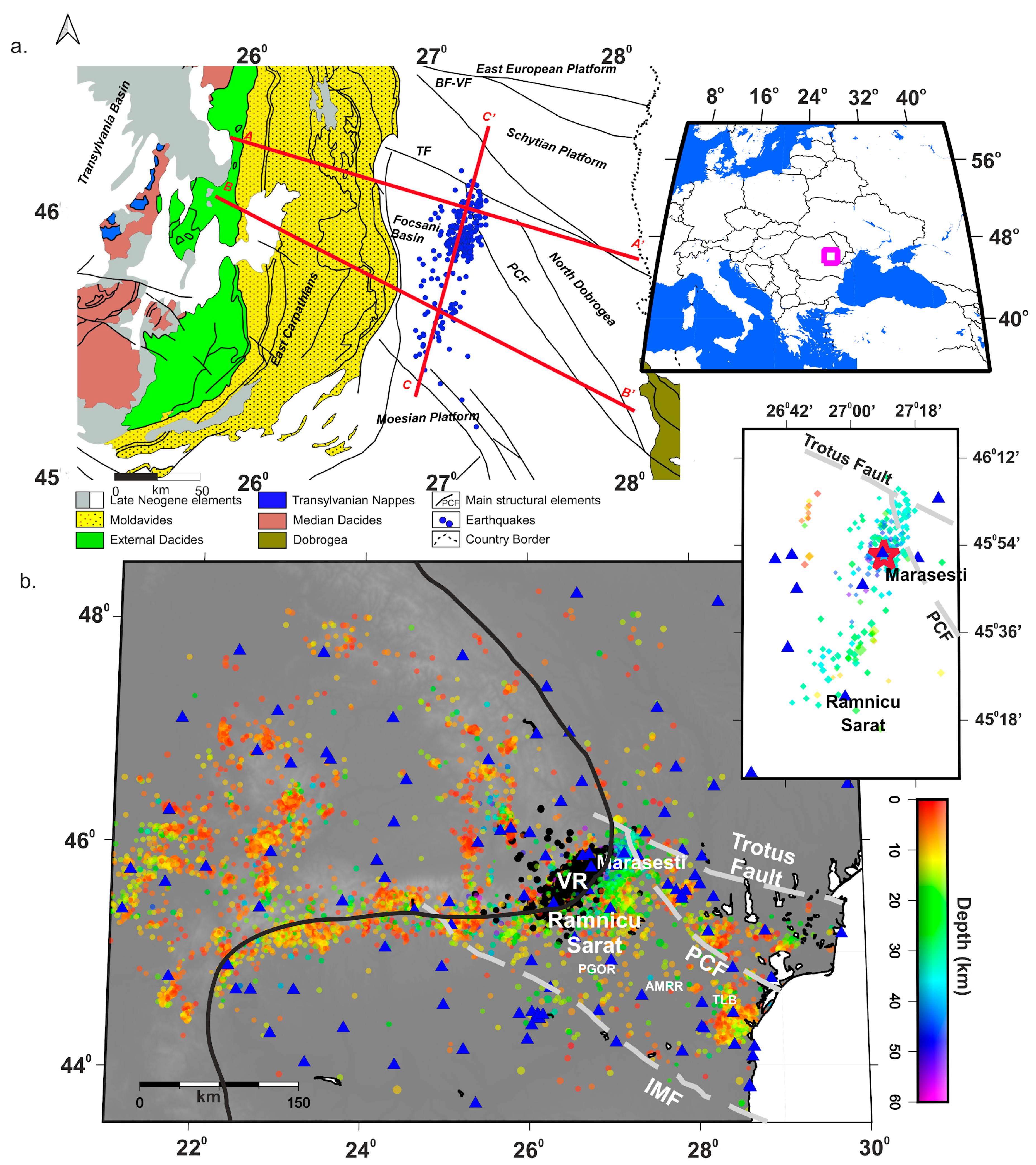
:1. Introduction
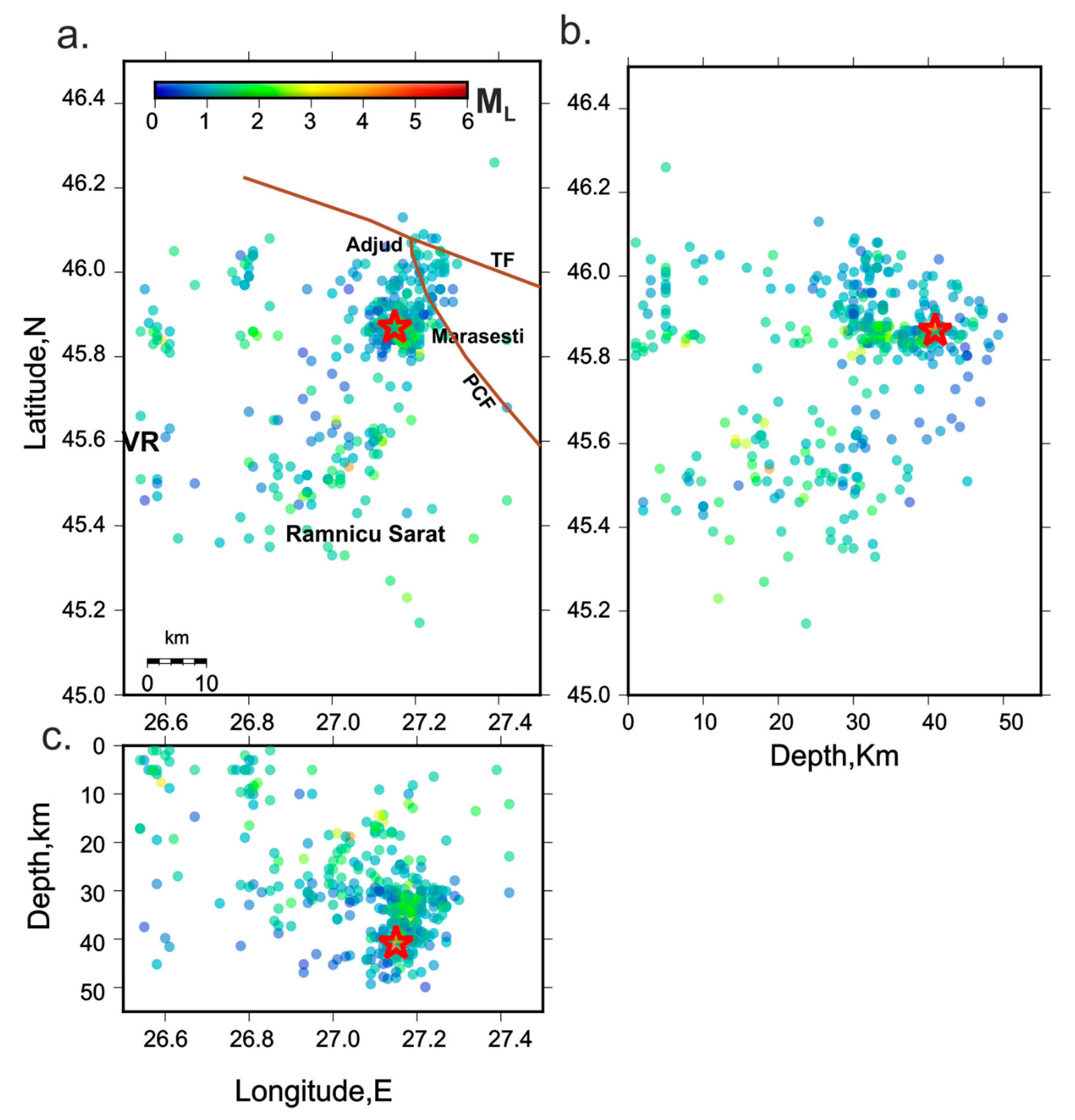
Sequence Description
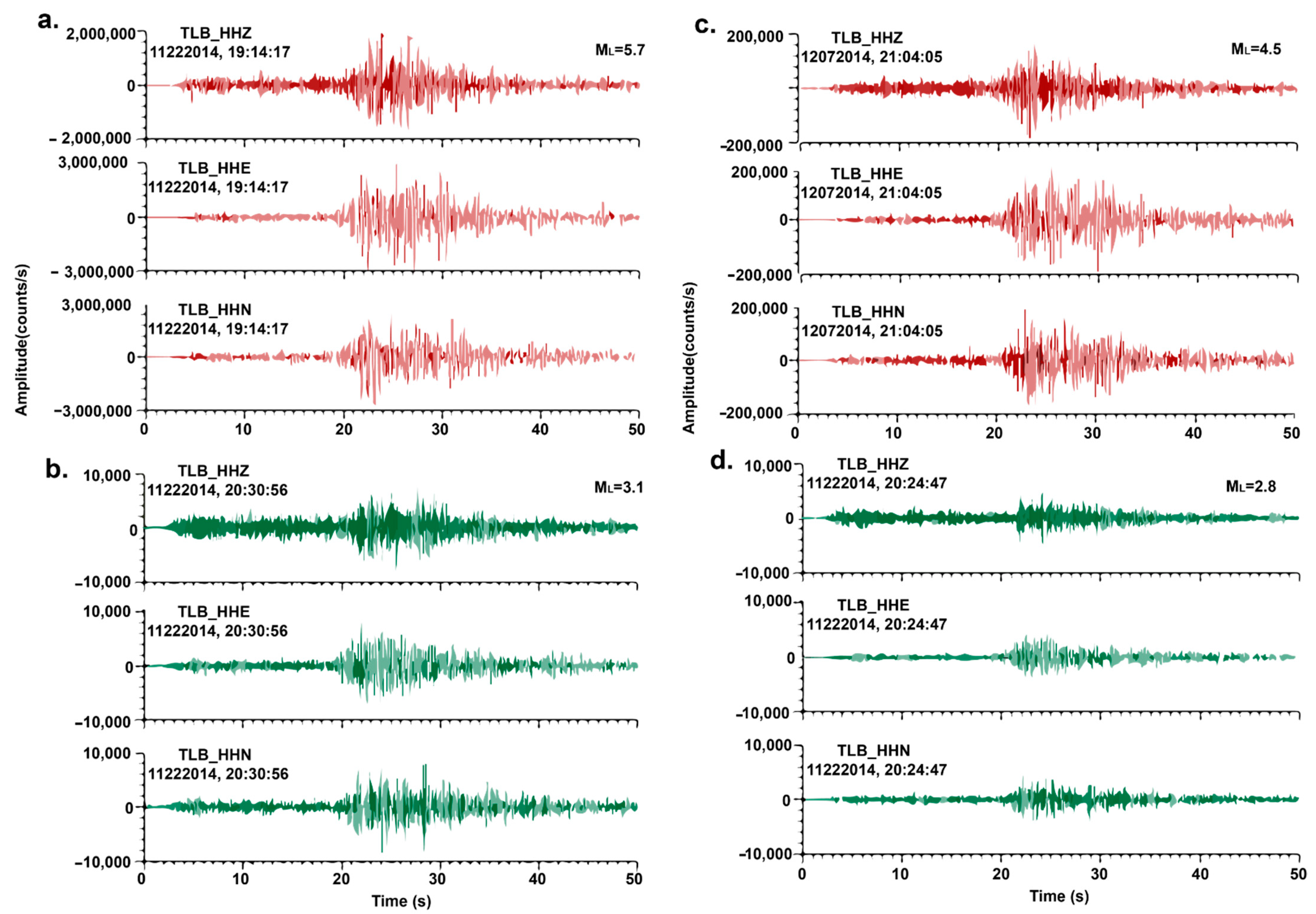
2. Methods and Data
3. Results
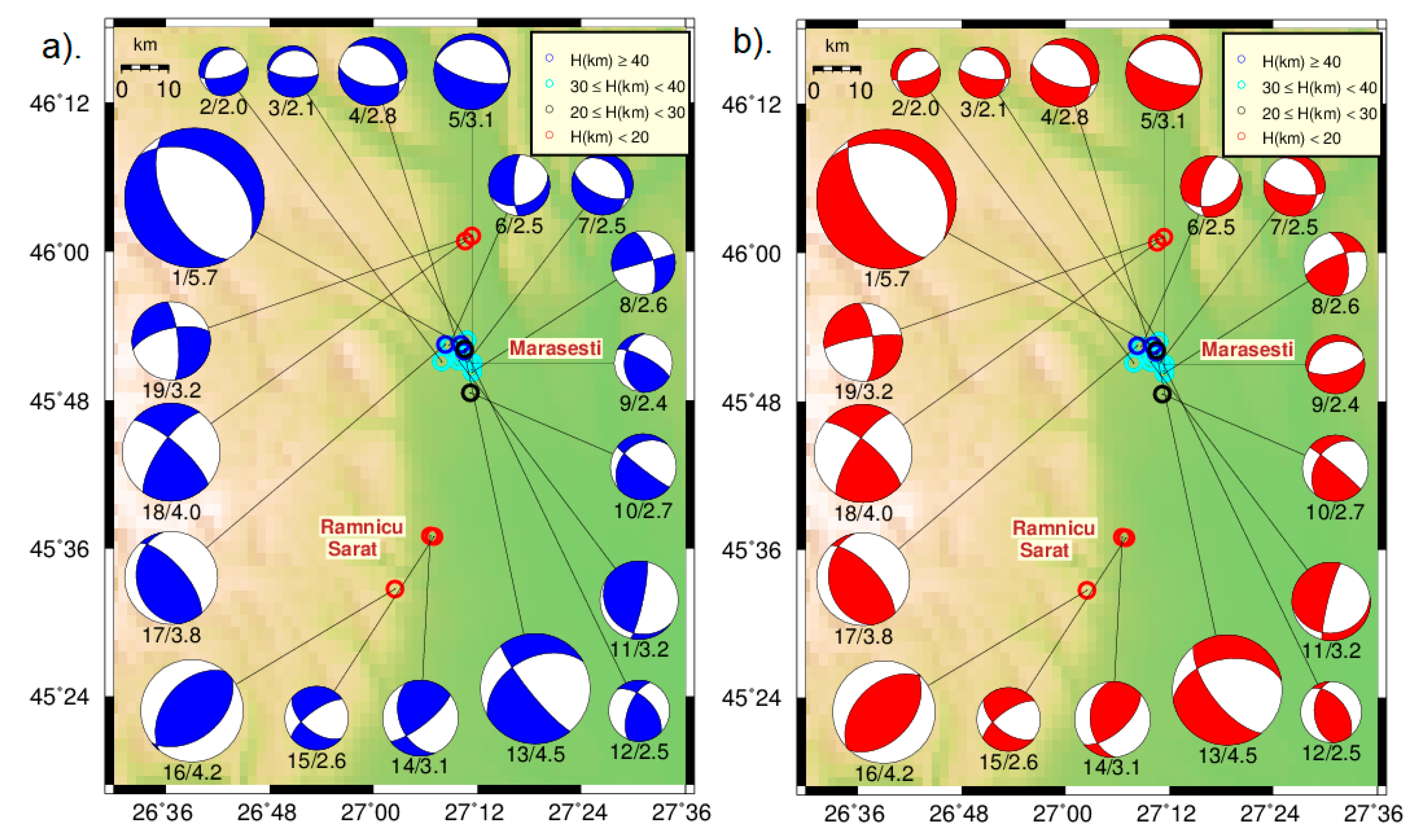
3.1. Focal Mechanisms
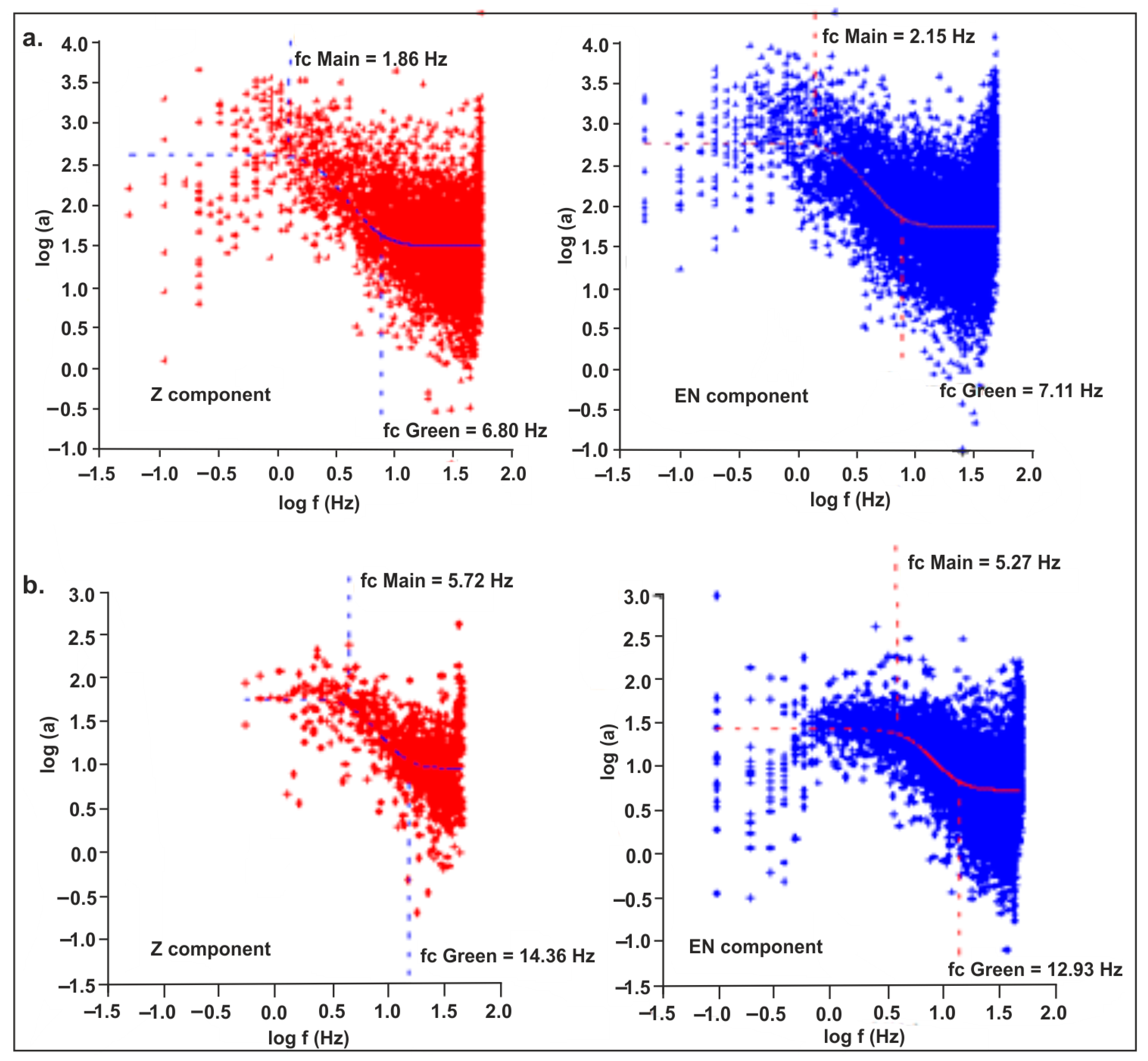
3.2. Spectral Ratios
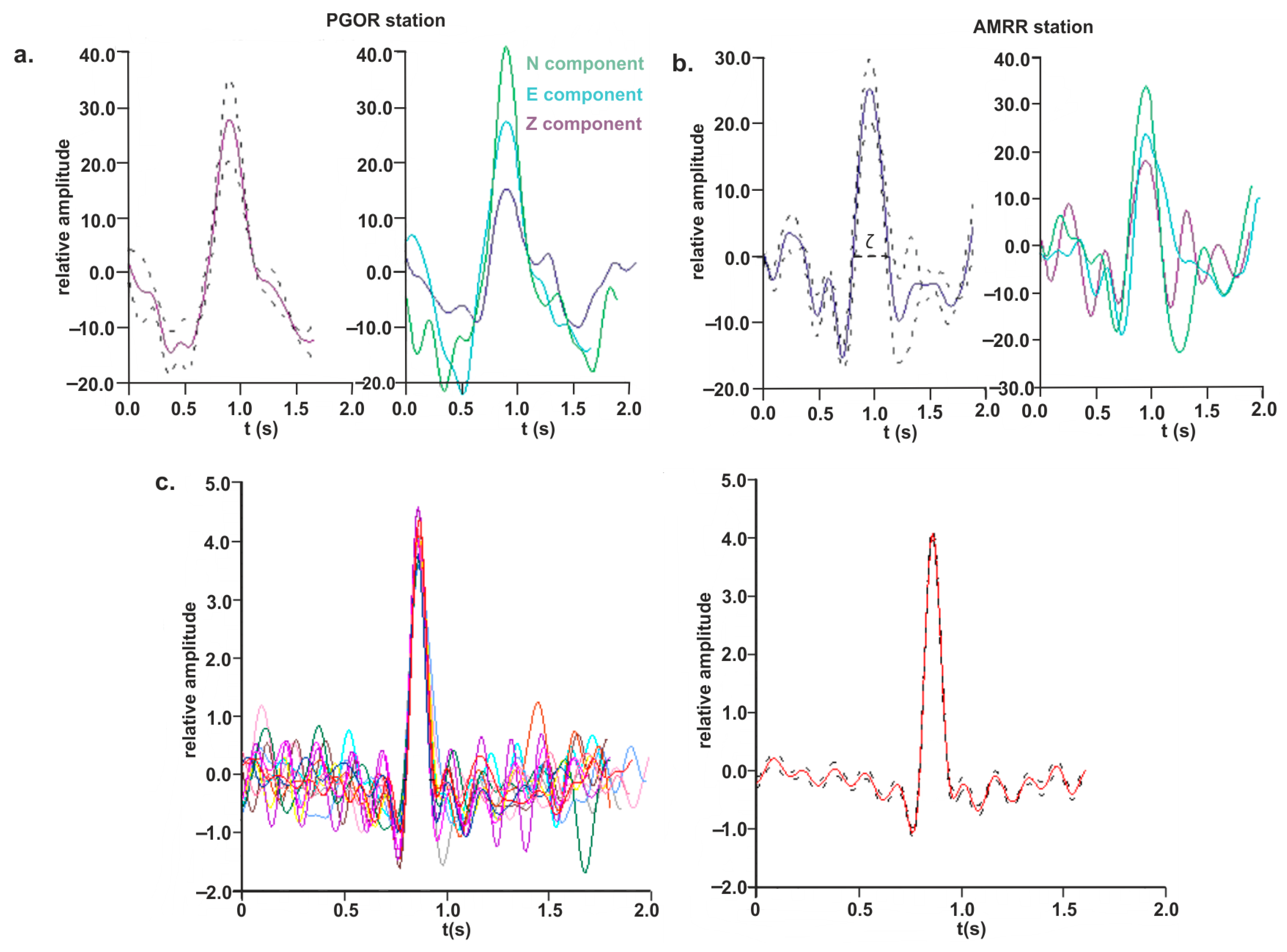
3.3. Empirical Green’s Function Analysis
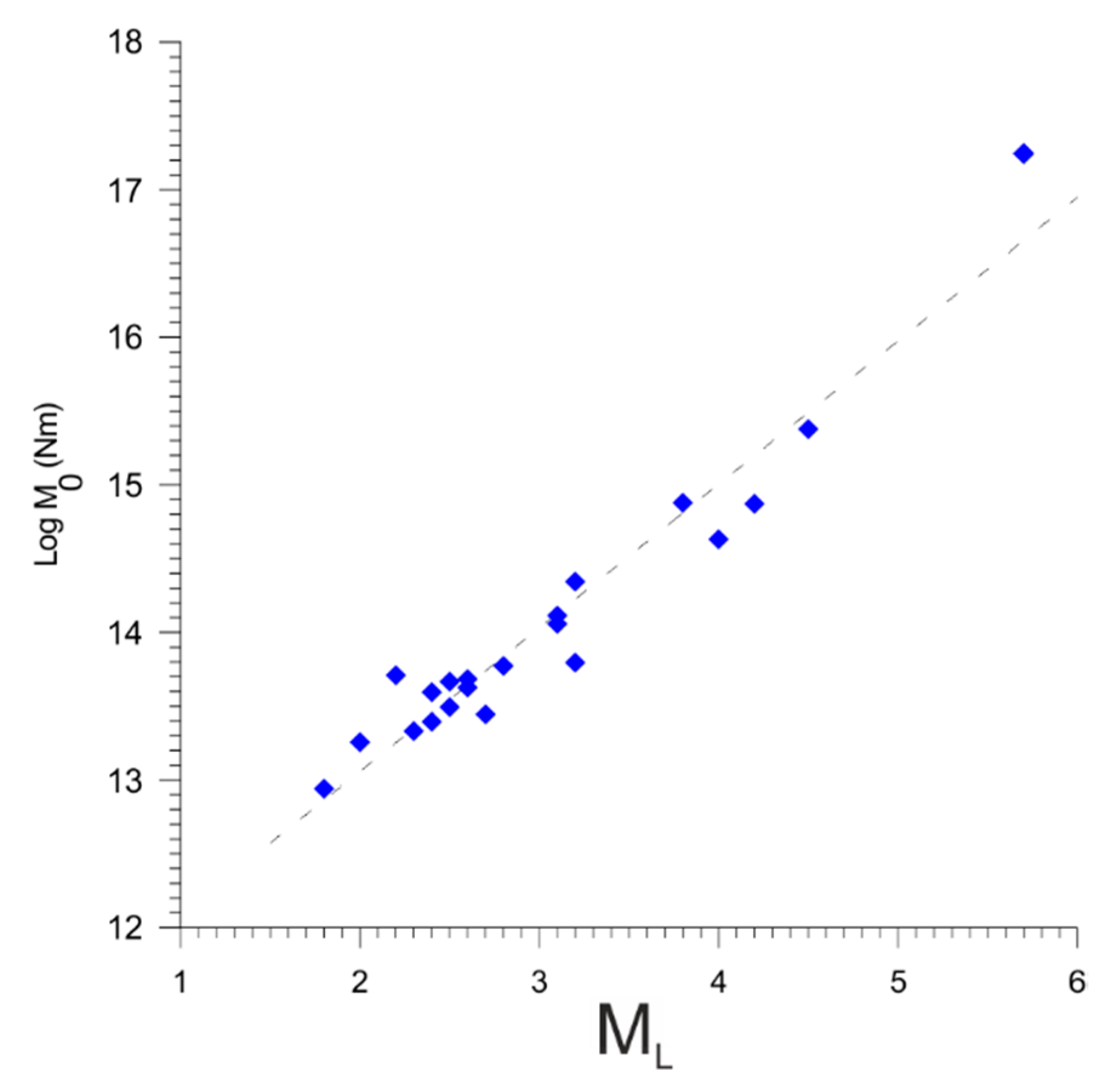
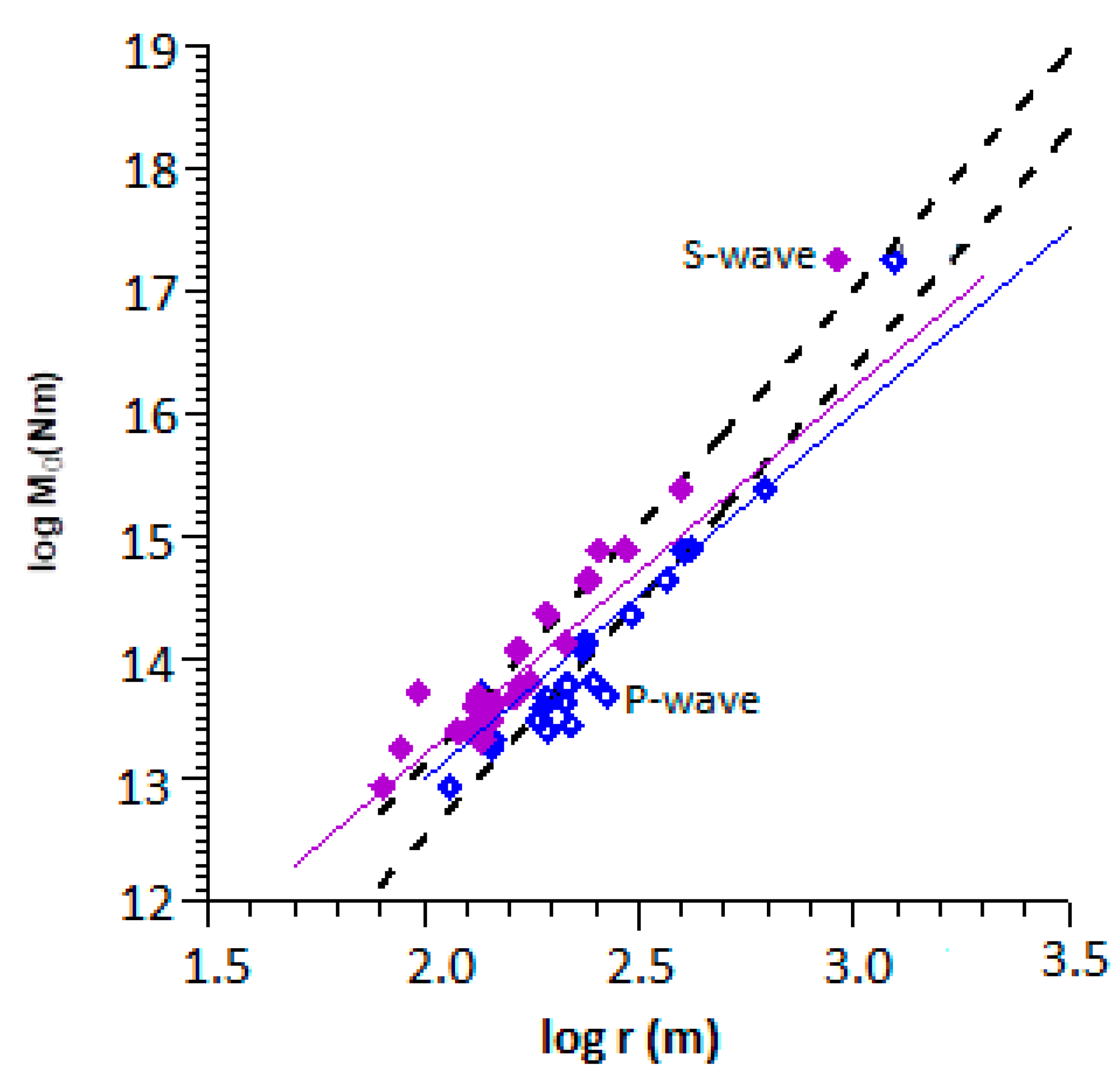
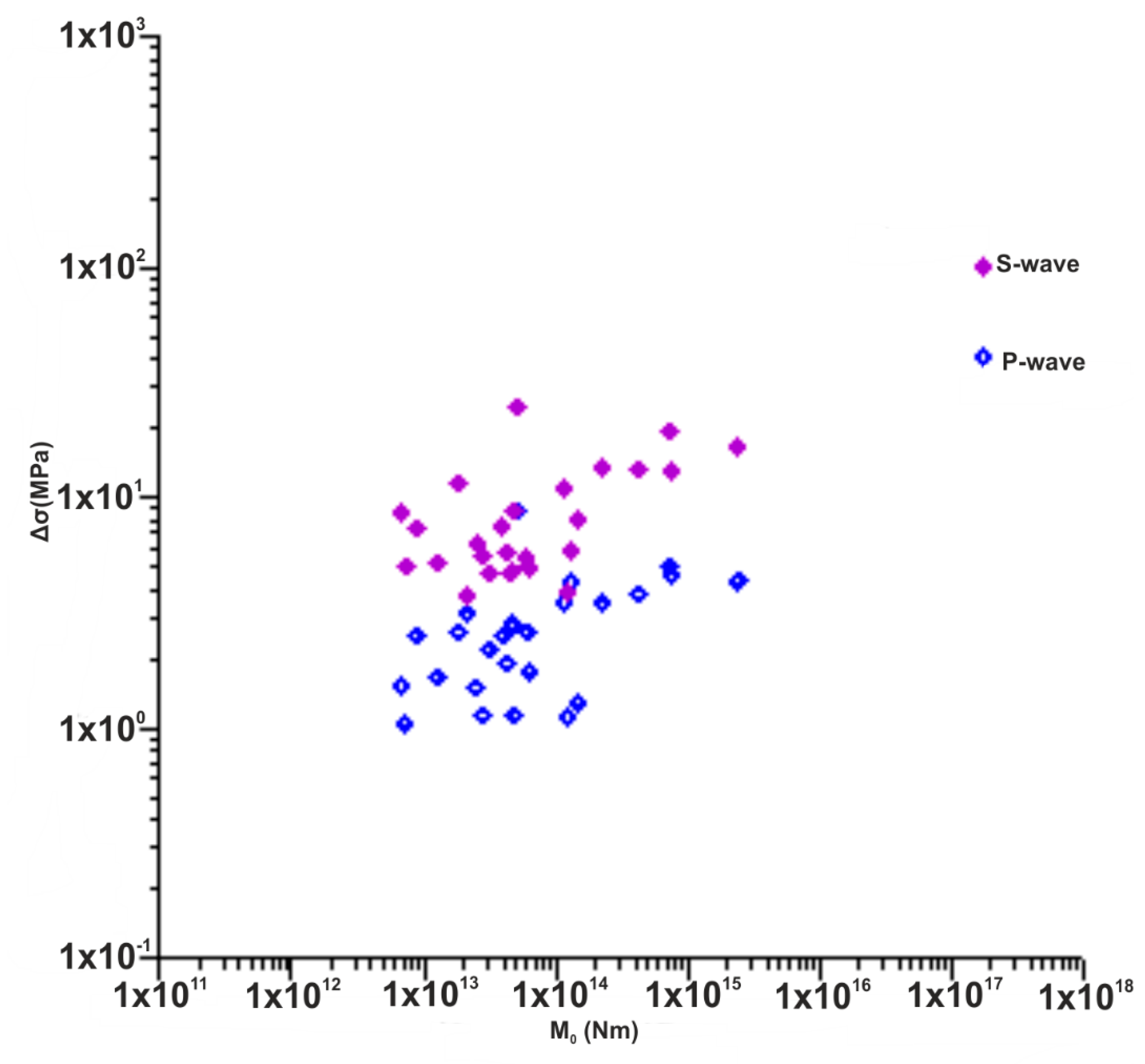
3.4. Scaling Relationships
3.5. Frequency–Magnitude Distribution
4. Discussion
5. Conclusions
Author Contributions
Funding
Institutional Review Board Statement
Informed Consent Statement
Data Availability Statement
Acknowledgments
Conflicts of Interest
References
- Mațenco, L.; Bertotti, G.; Leever, K.; Cloetingh, S.; Schmid, S.; Tărăpoancă, M.; Dinuc, C. Large-scale deformation in a locked collisional boundary: Interplay between subsidence and uplift, intraplate stress, and inherited lithospheric structure in the late stage of the SE Carpathians evolution. Tectonics 2007, 26, TC4011. [Google Scholar] [CrossRef] [Green Version]
- Bălă, A.; Toma-Danila, D.; Radulian, M. Focal mechanisms in Romania: Statistical features representative for earthquake-prone areas and spatial correlations with tectonic provinces. Acta Geod. Et Geophys. 2019, 54, 263–286. [Google Scholar] [CrossRef]
- Săndulescu, M. Geotectonics of Romania; Technical Publishing House: Bucharest, Romania, 1984. (In Romanian) [Google Scholar]
- Oncescu, M.C.; Mârza, V.; Rizescu, M.; Popa, M. The Romanian earthquakes catalogue between 984 and 1997. In Vrancea Earthquakes: Tectonics, Hazard. and Risk Mitigation; Wenzel, F., Lungu, D., Eds.; Kluwer Academic Publishers: Dordrecht, The Netherlands, 1999; pp. 43–47. [Google Scholar]
- Polonic, G. Structure of the crystalline basement in Romania. Rev. Roum. Geophys. 1996, 40, 57–69. [Google Scholar]
- Bălă, A.; Radulian, M.; Toma-Dănilă, D. Crustal stress partitioning in the complex seismic active areas of Romania. Acta Geod. Et Geohysica 2020, 55, 389–403. [Google Scholar] [CrossRef]
- Petrescu, L.; Borleanu, F.; Radulian, M.; Ismail-Zadeh, A.; Matenco, L. Tectonic regimes and stress patterns in the Vrancea Seismic Zone: Insights into intermediate depth earthquake nests in locked collisional settings. Tectonophysics 2020, 799, 228688. [Google Scholar] [CrossRef]
- Girbacea, R.; Frisch, W. Slab in the wrong place: Lower lithospheric mantle delamination in the last stage of the Eastern Carpathian subduction retreat. Geology 1998, 26, 611–614. [Google Scholar] [CrossRef]
- Cloetingh, S.; Burov, E.; Matenco, L.; Toussaint, G.; Bertotti, G.; Andriessen, P.A.M.; Wortel, M.J.R.; Spakman, W. Thermo-mechanical controls on the mode of continental collision in the SE Carpathians (Romania). Earth Planet. Sci. Lett. 2003, 6931, 1–20. [Google Scholar] [CrossRef]
- Seghedi, A.; Vaida, M.; Iordan, M.; Verniers, J. Paleozoic evolution of the Romanian part of the Moesian Platform: An overview. Geol. Belg. 2005, 8, 99–120. [Google Scholar]
- Matenco, L.; Munteanu, I.; ter Borgh, M.; Stanica, A.; Tilita, M.; Lericolais, G.; Dinu, C.; Oaie, G. The interplay between tectonics, sediment dynamics and gateways evolution in the Danube system from the Pannonian Basin to the western Black Sea. Sci. Total Environ. 2016, 543, 807–827. [Google Scholar] [CrossRef] [Green Version]
- Răileanu, V.; Tătaru, D.; Grecu, B. Crustal models in Romania–I. Moesian platform. Romanian Rep. Phys. 2012, 64, 539–554. [Google Scholar]
- Radulian, M.; Mandrescu, N.; Panza, G.; Popescu, E.; Utale, A. Characterization of seismogenic zones of Romania. Pure Appl. Geophys. 2000, 157, 57. [Google Scholar] [CrossRef]
- Bala, A.; Raileanu, V.; Dinu, C.; Diaconescu, M. Crustal seismicity and active fault systems in Romania. Rom. Rep. Phys. 2015, 67, 1176–1191. [Google Scholar]
- Ardeleanu, L.; Radulian, M.; Kravanja, S.; Dufumier, H.; Panza, G.F. Focal mechanism of earthquakes of Ramnicu Sarat (Romania) sequence of 21–22 February 1983 infered from waveform inversion. In Seismology in Europe; Thorkelsson, B., Ed.; European Seismological Commission (ESC): Reykjavik, Iceland, 1996; pp. 300–305. [Google Scholar]
- Popescu, E. Complex Study of the Earthquake Sequences on the Romanian Territory. Ph.D. Thesis, Institute of Atomic Physics, Bucharest, Romania, 2000; p. 281. [Google Scholar]
- Enescu, D.; Popescu, E.; Radulian, M. Source characteristics of Sinaia (Romania) sequence of May-June 1993. Tectonophysics 1996, 261, 39–49. [Google Scholar] [CrossRef]
- Enescu, D.; Popescu, E.; Radulian, M. Some parameters and scaling relations for Sinaia (Romania) earthquakes sequence of May -June, 1993. Rom. J. Phys. 1996, 41, 321–330. [Google Scholar]
- Popescu, E.; Placinta, A.O.; Radulian, M.; Borleanu, F.; Diaconescu, M.; Popa, M. Source parameters of the earthquake sequence that occurred close to the BURAR array (Romania) between 24 June and 1 July 2011. Ann. Geophys 2017, 60, S0225. [Google Scholar] [CrossRef] [Green Version]
- Demuth, A.; Tjåland, N.; Ottemöller, L. Earthquake source parameters in Norway determined with empirical Green’s functions. J. Seism. 2019, 23, 715–724. [Google Scholar] [CrossRef]
- Kanamori, H.; Anderson, D.L. Theoretical basis of some empirical relations in seismology. Bull. Seismol. Soc. Am. 1975, 65, 1073–1095. [Google Scholar]
- Scholz, C.H.; Aviles, C.A.; Wesnousky, S.G. Scaling differences between large interplate and intraplate earthquakes. Bull. Seimol. Soc. Am. 1986, 76, 65–70. [Google Scholar]
- Choy, G.L.; Boatwright, J.L. Global patterns of radiated seismic energy and apparent stress. J. Geophys. Res. 1995, 100, 18205–18228. [Google Scholar] [CrossRef] [Green Version]
- Popescu, E.; Radulian, M. Source characteristics of the seismic sequences in the Eastern Carpathians foredeep region (Romania). Tectonophysics 2001, 338, 325–337. [Google Scholar] [CrossRef]
- Popescu, E.; Neagoe, C.; Rogozea, M.; Moldovan, I.A.; Borleanu, F.; Radulian, M. Source parameters for the earthquake sequence occurred in the Ramnicu Sarat area (Romania) November-December 2007. Rom. J. Phys. 2011, 56, 265–278. [Google Scholar]
- Aki, K. Scaling law of seismic spectrum. J. Geophys. Res. 1967, 72, 1217–1231. [Google Scholar] [CrossRef]
- Shearer, P.M.; Prieto, G.A.; Hauksson, E. Comprehensive analysis of earthquake source spectra in southern California. J. Geophys. Res. 2006, 111, B06303. [Google Scholar] [CrossRef] [Green Version]
- Abercrombie, R.E.; Bannister, S.; Ristau, J.; Doser, D. Variability of earthquake stress drop in a subduction setting, the Hikurangi Margin, New Zealand. Geophys. J. Int. 2017, 208, 306–320. [Google Scholar] [CrossRef]
- Mori, J.; Abercrombie, R.E.; Kanamori, H. Stress drops and radiated energies of aftershocks of the 1994 Northridge, California, earthquake. J. Geophys. Res. Atmos. 2003, 108, 2545. [Google Scholar] [CrossRef] [Green Version]
- Havskov, J.; Ottemoller, L. Routine Data Processing in Earthquake Seismology; Springer: Berlin, Germany, 2010; p. 380. [Google Scholar]
- Constantin, A.P.; Moldovan, I.A.; Craiu, A.; Radulian, M.; Ionescu, C. Macroseismic intensity investigation of the November 2014, M=5.7, Vrancea (Romania) crustal earthquake. Ann. Geophys. 2016, 59, S0542. [Google Scholar] [CrossRef]
- Craiu, A.; Ghita, C.; Craiu, M.; Diaconescu, M.; Mihai, M.; Ardeleanu, L. Seismic events during the sequence of the moderate-size crustal earthquake of November 22, 2014 of Vrancea region (Romania). Ann. Geophys. 2019, 61, 6. [Google Scholar] [CrossRef]
- Mitrofan, H.; Chitea, F.; Anghelache, M.A.; Visan, M. Possible Triggered Seismicity Signatures Associated with the Vrancea Intermediate-Depth Strong Earthquakes (Southeast Carpathians, Romania). Seismol. Res. Lett. 2014, 85, 314–323. [Google Scholar] [CrossRef]
- Bratt, S.R.; Nagy, W. The LocSAT Program; Science Applications International Corporation: San Diego, CA, USA, 1991. [Google Scholar]
- Kennett, B.L.N.; Engdahl, E.R. Travel times for global earthquake location and phase identification. Geophys. J. Int. 1991, 105, 429–465. [Google Scholar] [CrossRef] [Green Version]
- Abercrombie, R.E. Investigating uncertainties in empirical Green’s function analysis of earthquake source parameters. J. Geophys. Res. Solid Earth 2015, 120, 4263–4277. [Google Scholar] [CrossRef]
- Havskov, J.; Ottemöller, L. SEISAN: The Earthquake Analysis Software; Version 7.2; University of Bergen: Bergen, Norway, 2001; p. 256. [Google Scholar]
- Snoke, J.A. Focmec: Focal mechanism determinations. Int. Geophys. 2003, 81, 1629–1630. [Google Scholar]
- Hardebeck, J.L.; Shearer, P.M. A new method for determining first motion focal mechanisms. Bull. Seismiol. Soc. Am. 2002, 92, 2264–2276. [Google Scholar] [CrossRef] [Green Version]
- Hardebeck, J.L.; Shearer, P.M. Using S/P Amplitude Ratios to Constrain the Focal Mechanisms of Small Earthquakes. Bull. Seismiol. Soc. Am. 2003, 93, 2434–2444. [Google Scholar] [CrossRef]
- Mueller, C.S. Source pulse enhancement by deconvolution of an empirical Green’s function. Geophys. Res. Lett. 1985, 12, 33–36. [Google Scholar] [CrossRef]
- Frankel, A.; Flechter, J.; Vernon, F.; Haar, L.; Berger, J.; Hanks, T.; Brune, J. Rupture characteristics and tomography source imaging of ML = 3 earthquakes near Anza, Southern California. J. Geophys. Res. 1986, 91, 12633–12650. [Google Scholar] [CrossRef]
- Hough, S.E.; Jacob, K.; Busby, R. Ground motions from a M = 3.5 earthquake near Massena, New York: Evidence for the poor resolution of corner frequency from small events. Seismiol. Res. Lett. 1989, 60, 95–99. [Google Scholar] [CrossRef]
- Mori, J.; Frankel, A. Source parameters for small events associated with the 1986 North Palm Springs, California earthquake determined using empirical Green functions. Bull. Seismiol. Soc. Am. 1990, 80, 278–285. [Google Scholar]
- Radulian, M.; Popescu, E.; Borleanu, F.; Diaconescu, M. December 2011–January 2012 seismic sequence in Southern Carpathians, Romania. Tectonophysics 2014, 623, 23–38. [Google Scholar] [CrossRef]
- Placinta, A.O.; Popescu, E.; Borleanu, F.; Radulian, M.; Popa, M. Analysis of source properties for the earthquake sequences in the South-Western Carpathians (Romania). Rom. Rep. Phys. 2016, 68, 1240–1258. [Google Scholar]
- Brune, J.N. Tectonic stress and the spectra of seismic shear waves from earthquakes. J. Geophys. Res. 1970, 75, 4997–5009. [Google Scholar] [CrossRef] [Green Version]
- Brune, J.N. Seismic sources, fault plane studies and tectonics. EOS 1971, 52, 178–187. [Google Scholar] [CrossRef]
- Aki, K.; Richards, P. Quantitative Seismology: Theory and Methods; Freeman: San Francisco, CA, USA, 1980; p. 932. [Google Scholar]
- Hanks, T.C.; Kanamori, H. A moment magnitude scale. J. Geophys. Res. 1979, 84, 2348–2350. [Google Scholar] [CrossRef]
- Gutenberg, R.; Richter, C.F. Frequency of earthquakes in California. Bull. Seismiol. Soc. Am. 1944, 34, 185–188. [Google Scholar]
- Wiemer, S. A Software Package to Analyze Seismicity: ZMAP. Seismiol. Res. Lett. 2001, 72, 373–382. [Google Scholar] [CrossRef]
- Aki, K. Maximum-likelihood estimate of b in the formula log N = a − bM and its confidence limits. Bull. Earthq. Res. Inst. Tokyo Univ. 1965, 43, 237–239. [Google Scholar]
- Radulian, M.; Popescu, E.; Bala, A.; Utale, A. Catalogue of the fault plane solutions for the earthquakes occurred on the Romanian territory. Rom. J. Phys. 2002, 47, 663–670. [Google Scholar]
- Ardeleanu, L. Reliability of source parameters of low magnitude crustal earthquakes of Vrancea retrieved by high frequency waveform inversion. Rom. J. Phys. 2011, 56, 827–841. [Google Scholar]
- Radulian, M.; Bala, A.; Popescu, E.; Toma-Danila, D. Earthquake mechanism and characterization of seismogenic zones in south-eastern part of Romania. Ann. Geophys. 2018, 61, 108. [Google Scholar] [CrossRef]
- Zoback, M.L. First- and Second-Order Patterns of Stress in the Lithosphere. The World Stress Map Project. J. Geophys. Res. 1992, 97, 11703–11728. [Google Scholar] [CrossRef]
- Radulian, M.; Popescu, E.; Plăcintă, A.O. Empirical Green’s function deconvolution applied for Vrancea earthquakes occurred in the last ten years. Environ. Eng. Manag. J. 2017, 16, 2605–2614. [Google Scholar] [CrossRef]
- Abercrombie, R.; Leavy, P. Source parameters of small earthquakes recorded at 2.5 km depth, Cajon Pass, southern California: Implications for earthquake scaling. Geophys. Res. Lett. 1993, 20, 1511–1514. [Google Scholar] [CrossRef]
- Molnar, P.; Fitch, T.J.; Wu, F.T. Fault plane solutions of shallow earthquakes and contemporary tectonics in Asia, Earth Planet. Sci. Lett. 1973, 19, 101–112. [Google Scholar]
- Prieto, G.A.; Shearer, P.M.; Vernon, F.L.; Kilb, D. Earthquake source scaling and self-similarity estimation from stacking p and s spectra. J. Geophys. Res. Solid Earth 2004, 109, B08310. [Google Scholar] [CrossRef]
- Viegas, G.L. Source parameters of the 16 July 2010 Mw 3.4 Germantown, Maryland, earthquake. Seism. Res. Lett. 2012, 83, 933–944. [Google Scholar] [CrossRef]
- Madariaga, R. Dynamics of an expanding circular crack. Bull. Seismiol. Soc. Am. 1976, 66, 639–666. [Google Scholar]
- Popescu, E.; Borleanu, F.; Rogozea, M.; Radulian, M. Source analysis for earthquake sequence occurred in Vrancea (Romania) region on 6 to 30 September 2008. Rom. Rep. Phys. 2012, 64, 571–590. [Google Scholar]
- Bindi, D.; Spallarossa, D.; Augliera, P.; Cattaneo, M. Source Parameters Estimated from the Aftershocks of the 1997 Umbria–Marche (Italy) Seismic Sequence. Bull. Seismiol. Soc. Am. 2001, 91, 448–455. [Google Scholar] [CrossRef]
- De Luca, G.; Scarpa, R.; Filippi, L.; Gorini, A.; Marcucci, S.; Marsan, P.; Milna, G.; Zambonelli, E. A detailed analysis of two seismic sequences in Abruzzo, central Apennines, Italy. J. Seism. 2000, 4, 1–21. [Google Scholar] [CrossRef]
- Fletcher, J.; Boatwright, J.; Haar, L.; Hanks, T.; McGarr, A. Source parameters for aftershocks of the Oroville, California, earthquake. Bull. Seismiol. Soc. Am. 1984, 74, 1101–1123. [Google Scholar]
- Lanza, V.; Spallarossa, D.; Cattaneo, M.; Bindi, D.; Augliera, P. Source parameters of small events using constrained deconvolution with empirical Green’s functions. Geophys. J. Int. 1999, 137, 651–662. [Google Scholar] [CrossRef] [Green Version]
- Detzel, H.A.; Bianchi, M.; Prieto, G.A.; Assumpção, M. Earthquake source properties of a shallow induced seismic sequence in SE Brazil. JGR Solid Earth 2017, 122, 2784–2797. [Google Scholar] [CrossRef]
- Tărăpoancă, M.; Bertotti, G.; Mațenco, L.; Dinu, C.; Cloetingh, S. Architecture of the Focsani depression: A 13 km deep basin in the Carpathians Bend Zone (Romania). Tectonics 2003, 22, 1074. [Google Scholar] [CrossRef]
- Stefănescu, M.; Stefanescu, M.; Polonic, P.; Alexandrescu, G.; Popescu, I.; Peliz, S.; Popescu, I.; Ionescu, F.; Niculin, M.; Popescu-Bradet, L.; et al. Geological cross Section. No. A 1-23; Institutul De Geologie Și Geofizică: Bucharest, Romania, 1988. [Google Scholar]
- Grad, M.; TIira, T.; ESC Working Group. The Moho depth map of the European Plate. Geophys. J. Int. 2009, 176, 279–292. [Google Scholar] [CrossRef] [Green Version]
- Popescu, E.; Grecu, B.; Popa, M.; Rizescu, M.; Radulian, M. Seismic source properties: Indications of lithosphere irregular structure on depth beneath Vrancea region. Rom. Rep. Phys. 2003, 55, 458–509. [Google Scholar]
- Mărmureanu, A.; Ionescu, C.; Grecu, B.; Toma-Danila, D.; Tiganescu, A.; Neagoe, C.; Toader, V.; Craifaleanu, I.G.; Dragomir, C.S.; Meiţă, V.; et al. From National to Transnational Seismic Monitoring Products and Services in the Republic of Bulgaria, Republic of Moldova, Romania, and Ukraine. Seismiol. Res. Lett. 2021, XX, 1–19. [Google Scholar] [CrossRef]
- Radulescu, D.P.; Cornea, I.; Sandulescu, M.; Constantinescu, P.; Pompilian, A. Structure de la croute terrestre en Roumanie, Essai d’interpretation des etudes sismiques profondes. Anu. Inst. Geol. Geofiz. L. 1976, 50, 5–36. [Google Scholar]
- Visarion, M.; Săndulescu, M.; Stănică, D.; Atanasiu, L. An improved geotectonic model of the East Carpathians. Rev. Roum. Geol. Geophys Et Geogr. Ser. Geophys. 1988, 32, 43–52. [Google Scholar]
- Leever, K.; Maţenco, L.; Bertotti, G.; Cloetingh, S.; Drijkoningen, K.G.; Vasiliev, I. Pliocene to Recent kinematics in the Focşani basin, Romania: New constraints from shallow seismic and paleomagnetic data. Basin Res. 2006, 18, 521–545. [Google Scholar] [CrossRef]
- Frohlich, C.; Davis, S.D. Teleseismic b values; or, much ado about 1.0. J. Geophys. Res. 1993, 98, 631–644. [Google Scholar] [CrossRef]
- Schorlemmer, D.; Wiemer, S.; Wyss, M. Variations in earthquake-size distribution across different stress regimes. Nature 2005, 437, 539–542. [Google Scholar] [CrossRef]
- Öztürk, S. A study on the correlations between seismotectonic bvalue and Dc-value, and seismic quiescence Z-value in the Western Anatolian region of Turkey. Mitt. Osterr. Geol. Ges. 2015, 108, 172–184. [Google Scholar]
- Borleanu, F.; Petrescu, L.; Enescu, B.; Popa, M.; Radulian, M. The missing craton edge: Crustal structure of the East European Craton beneath the Carpathian Orogen revealed by double-difference tomography. Glob. Planet. Chang. 2021, 197, 103390. [Google Scholar] [CrossRef]
- Twiss, R.J.; Moores, E.M. Structural Geology; W.H. Freeman & Co.: San Francisco, CA, USA, 1992; p. 532. [Google Scholar]
- Matenco, L.; Bertotti, G.; Cloetingh, S.; Dinu, C. Subsidence analysis and tectonic evolution of the external Carpathian–Moesian Platform region during Neogene times. Sediment. Geol. 2003, 156, 71–94. [Google Scholar] [CrossRef]
- Ţugui, A.; Craiu, M.; Rogozea, M.; Popa, M.; Radulian, M. Earth physics seismotectonics of Vrancea (Romania) zone: The case of crustal seismicity in the foredeep area. Rom. Rep. Phys. 2009, 61, 325–334. [Google Scholar]
- Răileanu, V.; Dinu, C.; Ardeleanu, L.; Diaconescu, V.; Popescu, E.; Bălă, A. Crustal seismicity and associated fault systems in Romania. Cah. Du Cent. Eur. De Géodynamique Et De Séismologie 2009, 28, 153–159. [Google Scholar]
- Tanırcan, G.; Miyake, H.; Yamanaka, H.; Ozel, O. Large Stress Release During Normal-Faulting Earthquakes in Western Turkey Supported by Broadband Ground Motion Simulations. Pure Appl. Geophys. 2020, 177, 1969–1981. [Google Scholar] [CrossRef]
- Baltay, A.; Ide, S.; Prieto, G.; Beroza, G. Variability in earthquake stress drop and apparent stress. Geophys. Res. Lett. 2011, 38, L06303. [Google Scholar] [CrossRef] [Green Version]


| No | Date DDMMYYYY | OriginTime hh:mm:ss | Latitude (°N) | Longitude (°E) | Depth (km) | ML |
|---|---|---|---|---|---|---|
| M1 | 22112014 | 19:14:17 | 45.8683 | 27.1517 | 41 | 5.7 |
| M2 | 22112014 | 20:30:56 | 45.8530 | 27.1859 | 36 | 3.1 |
| M3 | 07122014 | 21:04:05 | 45.8836 | 27.1714 | 41 | 4.5 |
| M4 | 12012015 | 06:08:31 | 45.5420 | 27.0448 | 19 | 4.2 |
| M5 | 19012015 | 23:53:07 | 45.8782 | 27.1483 | 40 | 3.8 |
| M6 | 29062015 | 22:20:56 | 46.0114 | 27.1754 | 19 | 4.0 |
| 1 | 22112014 | 19:27:39 | 45.8688 | 27.1185 | 40 | 2.0 |
| 2 | 22112014 | 20:24:47 | 45.8626 | 27.1644 | 34 | 2.8 |
| 3 | 22112014 | 20:30:56 | 45.8530 | 27.1859 | 36 | 3.1 |
| 4 | 23112014 | 01:14:39 | 45.8819 | 27.1610 | 35 | 2.5 |
| 5 | 23112014 | 02:21:05 | 45.8509 | 27.1852 | 34 | 2.5 |
| 6 | 23112014 | 04:01:58 | 45.8230 | 27.1750 | 31 | 2.6 |
| 7 | 23112014 | 05:27:58 | 45.8450 | 27.1889 | 35 | 2.4 |
| 8 | 23112014 | 23:22:49 | 45.8477 | 27.1852 | 33 | 2.3 |
| 9 | 24112014 | 00:45:06 | 45.8700 | 27.1660 | 34 | 2.4 |
| 10 | 25112014 | 01:52:25 | 45.8480 | 27.1612 | 39 | 3.2 |
| 11 | 07122014 | 21:04:05 | 45.8836 | 27.1714 | 41 | 4.5 |
| 12 | 14122014 | 17:24:47 | 45.6054 | 27.1018 | 14 | 3.1 |
| 13 | 14122014 | 18:24:34 | 45.6036 | 27.1164 | 16 | 2.6 |
| 14 | 18012015 | 22:41:40 | 45.4962 | 27.0243 | 31 | 1.8 |
| 15 | 19012015 | 23:53:07 | 45.8782 | 27.1483 | 40 | 3.8 |
| 16 | 20012015 | 02:52:46 | 45.8850 | 27.1585 | 33 | 2.2 |
| 17 | 01072015 | 04:34:24 | 46.0217 | 27.1893 | 17 | 3.2 |
| Crt. No. | Date DDMMYYYY | Origin Time hh:mm:ss | ML | FOCMEC | HASH | No. of Polarities/ No. of Amplitude Ratios | Type of Fault Plane | ||||
|---|---|---|---|---|---|---|---|---|---|---|---|
| Strike | Dip | Rake | Strike | Dip | Rake | ||||||
| AF | NBP | NBAR | FPU | AFPU | F-Fit STDR | ||||||
| 1 | 22112014 | 19:14:17 | 5.7 | 152 | 55 | −75 | 305 | 27 | −110 | 48/11 | NF |
| 0.08 | 3 | 5 | 1.10 | 1.80 | 0.06 | ||||||
| 0.40 | |||||||||||
| 2 | 22112014 | 19:27:39 | 2.0 | 77 | 71 | −69 | 207 | 30 | −134 | 12/6 | NF |
| 0.19 | 3 | 4 | 2.00 | 2.40 | 0.28 | ||||||
| 0.69 | |||||||||||
| 3 | 22112014 | 19:32:37 | 2.1 | 96 | 72 | −81 | 100 | 72 | −109 | 13/7 | NF |
| 0.18 | 1 | 4 | 11.30 | 13.50 | 0.19 | ||||||
| 0.65 | |||||||||||
| 4 | 22112014 | 20:24:47 | 2.8 | 315 | 40 | −61 | 106 | 60 | −110 | 24/13 | NLLO |
| 0.20 | 1 | 1 | 2.80 | 0.00 | 0.09 | ||||||
| 0.67 | |||||||||||
| 5 | 22112014 | 20:30:56 | 3.1 | 287 | 1 | −90 | 109 | 75 | −91 | 24/6 | NF |
| 0.17 | 0 | 2 | 2.80 | 3.10 | 0.05 | ||||||
| 0.51 | |||||||||||
| 6 | 23112014 | 01:14:39 | 2.5 | 70 | 36 | −26 | 192 | 65 | −120 | 21/5 | NLLO |
| 0.11 | 1 | 3 | 6.50 | 5.30 | 0.21 | ||||||
| 0.71 | |||||||||||
| 7 | 23112014 | 02:21:05 | 2.5 | 327 | 33 | −62 | 102 | 68 | −116 | 22/4 | NLLO |
| 0.15 | 3 | 2 | 0.60 | 1.00 | 0.11 | ||||||
| 0.72 | |||||||||||
| 8 | 23112014 | 04:01:58 | 2.6 | 344 | 64 | 0 | 248 | 71 | 146 | 19/6 | SS |
| 0.12 | 1 | 2 | 6.40 | 5.00 | 0.04 | ||||||
| 0.6 | |||||||||||
| 9 | 23112014 | 05:27:58 | 2.4 | 298 | 73 | 58 | 244 | 26 | −103 | 16/2 | RLLO |
| 0.16 | 2 | 1 | 4.70 | 9.10 | 0.15 | ||||||
| 0.68 | |||||||||||
| 10 | 23112014 | 10:16:15 | 2.7 | 128 | 85 | −60 | 215 | 40 | 174 | 19/7 | NLLO |
| 0.13 | 1 | 3 | 10.40 | 17.20 | 0.07 | ||||||
| 0.48 | |||||||||||
| 11 | 25112014 | 01:52:25 | 3.2 | 127 | 18 | 26 | 8 | 20 | −21 | 23/2 | RLLO |
| 0.04 | 1 | 1 | 5.10 | 15.90 | 0.15 | ||||||
| 0.72 | |||||||||||
| 12 | 02122014 | 04:19:29 | 2.5 | 315 | 54 | 37 | 177 | 44 | 117 | 12/6 | RLLO |
| 0.17 | 1 | 3 | 17.60 | 3.20 | 0.20 | ||||||
| 0.65 | |||||||||||
| 13 | 07122014 | 21:04:05 | 4.5 | 141 | 81 | −47 | 260 | 43 | −144 | 45/11 | NLLO |
| 0.11 | 4 | 6 | 10.40 | 8.10 | 0.17 | ||||||
| 0.70 | |||||||||||
| 14 | 14122014 | 17:24:47 | 3.1 | 158 | 44 | 22 | 48 | 62 | 121 | 28/7 | RLLO |
| 0.19 | 2 | 1 | 5.10 | 2.10 | 0.16 | ||||||
| 0.63 | |||||||||||
| 15 | 14122014 | 18:24:34 | 2.6 | 129 | 55 | −24 | 234 | 68 | −143 | 17/4 | NLLO |
| 0.14 | 1 | 1 | 5.20 | 1.90 | 0.09 | ||||||
| 0.57 | |||||||||||
| 16 | 12012015 | 06:08:31 | 4.2 | 220 | 45 | 82 | 226 | 45 | 93 | 36/5 | RF |
| 0.14 | 6 | 2 | 1.50 | 1.00 | 0.18 | ||||||
| 0.62 | |||||||||||
| 17 | 19012015 | 23:53:07 | 3.8 | 319 | 67 | 77 | 169 | 27 | 119 | 42/6 | RF |
| 0.16 | 2 | 1 | 3.30 | 2.20 | 0.05 | ||||||
| 0.73 | |||||||||||
| 18 | 29062015 | 22:20:56 | 4.0 | 311 | 74 | 20 | 214 | 72 | 161 | 43/11 | RLLO |
| 0.21 | 2 | 7 | 9.20 | 3.00 | 0.05 | ||||||
| 0.69 | |||||||||||
| 19 | 01072015 | 04:34:24 | 3.2 | 257 | 64 | −16 | 354 | 69 | −170 | 26/6 | LLSS |
| 0.25 | 1 | 2 | 14.70 | 4.30 | 0.07 | ||||||
| 0.46 | |||||||||||
| Earthquake Pair | Epicenters Inter-Distance (km) | Hypocenters Inter-Distance (km) | Depths Distance (km) | ML Difference |
|---|---|---|---|---|
| M1-1 | 2.6 | 2.9 | 1.4 | 3.7 |
| M1-2 | 1.2 | 6.6 | 6.5 | 2.9 |
| M1-3 | 3.1 | 5.6 | 4.6 | 2.6 |
| M1-4 | 1.7 | 6.3 | 6.1 | 3.2 |
| M1-5 | 3.2 | 7.4 | 6.7 | 3.2 |
| M1-6 | 5.3 | 11.2 | 9.9 | 3.1 |
| M1-8 | 5.3 | 9.3 | 7.6 | 3.4 |
| M1-10 | 2.4 | 3.2 | 2.1 | 2.5 |
| M1-11 | 2.3 | 2.3 | 0.3 | 1.2 |
| M1-15 | 1.1 | 1.6 | 1.1 | 1.9 |
| M1-16 | 1.9 | 7.7 | 7.5 | 3.5 |
| M2-1 | 5.5 | 6.4 | 3.2 | 1.1 |
| M3-1 | 4.4 | 4.5 | 1.1 | 2.5 |
| M3-2 | 2.4 | 6.6 | 6.2 | 1.7 |
| M3-3 | 3.6 | 5.6 | 4.3 | 1.4 |
| M3-4 | 0.8 | 5.9 | 5.8 | 2.0 |
| M3-5 | 3.8 | 7.4 | 6.4 | 2.0 |
| M3-6 | 6.7 | 11.7 | 9.6 | 1.9 |
| M3-7 | 4.5 | 7.5 | 6.0 | 2.1 |
| M3-8 | 6.7 | 9.9 | 7.3 | 2.2 |
| M3-9 | 1.6 | 6.4 | 6.2 | 2.1 |
| M3-10 | 4.0 | 4.4 | 1.8 | 1.3 |
| M3-16 | 1.0 | 7.3 | 7.2 | 2.3 |
| M4-12 | 8.6 | 9.7 | 4.5 | 1.1 |
| M4-13 | 8.8 | 9.3 | 3.1 | 1.6 |
| M4-14 | 5.3 | 15.8 | 14.9 | 2.4 |
| M5-1 | 2.5 | 2.5 | 0.3 | 1.8 |
| M5-2 | 2.1 | 5.8 | 5.4 | 1.0 |
| M5-7 | 4.8 | 7.1 | 5.2 | 1.4 |
| M5-9 | 1.6 | 5.6 | 5.4 | 1.4 |
| M5-16 | 1.1 | 6.5 | 6.4 | 1.6 |
| M6-17 | 1.4 | 1.9 | 1.3 | 0.8 |
| No. of ev. | fcP (Hz) | fcS (Hz) | fcP/fcS |
|---|---|---|---|
| M1 | 1.92 | 2.04 | 0.94 |
| M2 | 9.25 | 8.72 | 1.06 |
| M3 | 3.81 | 3.98 | 0.96 |
| M4 | 4.46 | 4.69 | 0.95 |
| M5 | 5.67 | 5.38 | 1.05 |
| M6 | 5.13 | 5.20 | 0.99 |
| 1 | 16.44 | 17.98 | 0.91 |
| 2 | 10.07 | 8.62 | 1.17 |
| 3 | 3.81 | 3.98 | 0.96 |
| 4 | 11.14 | 8.86 | 1.26 |
| 5 | 11.75 | 10.12 | 1.16 |
| 6 | 9.21 | 8.96 | 1.03 |
| 7 | 11.47 | 10.97 | 1.05 |
| 8 | 15.00 | 10.61 | 1.41 |
| 9 | 11.15 | 12.08 | 0.92 |
| 10 | 6.48 | 6.79 | 0.95 |
| 11 | 3.81 | 3.98 | 0.96 |
| 12 | 8.25 | 6.10 | 1.35 |
| 13 | 7.30 | 9.69 | 0.75 |
| 14 | 17.06 | 16.45 | 1.04 |
| 15 | 5.67 | 5.38 | 1.05 |
| 16 | 15.83 | 14.91 | 1.06 |
| 17 | 7.20 | 6.80 | 1.06 |
| Event | Seismic Moment (Nm) | Mw | Source Radius (m) | Stress Drop (MPa) | ||
|---|---|---|---|---|---|---|
| fcP (Hz) | fcS (Hz) | fcP | fcS | |||
| M1 | 1.76 × 10¹⁷ | 5.4 | 1236 | 914 | 41.0 | 101.0 |
| M2 | 1.14 × 10¹⁴ | 2.7 | 234 | 166 | 3.5 | 11.0 |
| M3 | 2.39 × 10¹⁵ | 3.4 | 622 | 397 | 4.4 | 16.7 |
| M4 | 7.43 × 10¹⁴ | 3.3 | 402 | 256 | 5.0 | 19.4 |
| M5 | 7.55 × 10¹⁴ | 3.1 | 417 | 294 | 4.6 | 13.0 |
| M6 | 4.28 × 10¹⁴ | 3.2 | 366 | 241 | 3.8 | 13.4 |
| Date DDMMYYYY | Origin Time hh:mm:ss | Seismic Moment (Nm) | Mw | Source Radius (m) | Stress Drop (MPa) | ||
|---|---|---|---|---|---|---|---|
| from fcP | from fcS | P | S | ||||
| 22112014 | 19:27:39 | 1.80 × 10¹³ | 2.1 | 144 | 88 | 2.6 | 11.6 |
| 22112014 | 20:24:47 | 5.92 × 10¹³ | 2.6 | 215 | 168 | 2.6 | 5.5 |
| 22112014 | 20:30:56 | 1.14 × 10¹⁴ | 2.7 | 234 | 166 | 3.5 | 11.0 |
| 23112014 | 01:14:39 | 4.63 × 10¹³ | 2.4 | 194 | 163 | 2.8 | 4.7 |
| 23112014 | 02:21:05 | 3.11 × 10¹³ | 2.4 | 184 | 143 | 2.2 | 4.7 |
| 23112014 | 04:01:58 | 4.23× 10¹³ | 2.5 | 213 | 147 | 1.9 | 5.8 |
| 23112014 | 05:27:58 | 3.93 × 10¹³ | 2.3 | 189 | 132 | 2.5 | 7.5 |
| 23112014 | 23:22:49 | 2.14 × 10¹³ | 2.3 | 144 | 136 | 3.1 | 3.7 |
| 24112014 | 00:45:06 | 2.48 × 10¹³ | 2.3 | 194 | 120 | 1.5 | 6.3 |
| 25112014 | 01:52:25 | 2.21 × 10¹⁴ | 2.8 | 303 | 193 | 3.5 | 13.5 |
| 07122014 | 21:04:05 | 2.39× 10¹⁵ | 3.4 | 622 | 397 | 4.4 | 16.7 |
| 14122014 | 17:24:47 | 1.30 × 10¹⁴ | 2.7 | 236 | 213 | 4.3 | 5.9 |
| 14122014 | 18:24:34 | 4.83 × 10¹³ | 2.5 | 266 | 134 | 1.1 | 8.8 |
| 18012015 | 22:41:40 | 8.71 × 10¹² | 2.0 | 115 | 80 | 2.5 | 7.4 |
| 19012015 | 23:53:07 | 7.55 × 10¹⁴ | 3.1 | 417 | 294 | 4.6 | 13.0 |
| 20012015 | 02:52:46 | 5.12 × 10¹³ | 2.2 | 137 | 98 | 8.7 | 24.5 |
| 01072015 | 04:34:24 | 6.24× 10¹³ | 2.8 | 249 | 176 | 1.8 | 5.0 |
| Event | Seismic Moment (Nm) | Mw | τ (s) | fc (Hz) | Source Radius (m) | Stress Drop (MPa) |
|---|---|---|---|---|---|---|
| τ | τ | |||||
| M1 | 1.76 × 10¹⁷ | 5.4 | 0.5 | 1.27 | 666 | 260.7 |
| M2 | 1.14 × 10¹⁴ | 2.7 | 0.16 | 3.98 | 213 | 5.2 |
| M3 | 2.39 × 10¹⁵ | 3.4 | 0.26 | 2.45 | 346 | 25.2 |
| M4 | 7.43 × 10¹⁴ | 3.3 | 0.18 | 3.54 | 240 | 23.6 |
| M5 | 7.55 × 10¹⁴ | 3.1 | 0.23 | 2.77 | 306 | 11.5 |
| M6 | 4.28 × 10¹⁴ | 3.2 | 0.22 | 2.90 | 293 | 7.4 |
Publisher’s Note: MDPI stays neutral with regard to jurisdictional claims in published maps and institutional affiliations. |
© 2021 by the authors. Licensee MDPI, Basel, Switzerland. This article is an open access article distributed under the terms and conditions of the Creative Commons Attribution (CC BY) license (https://creativecommons.org/licenses/by/4.0/).
Share and Cite
Placinta, A.O.; Borleanu, F.; Popescu, E.; Radulian, M.; Munteanu, I. Earthquake Source Properties of a Lower Crust Sequence and Associated Seismicity Perturbation in the SE Carpathians, Romania, Collisional Setting. Acoustics 2021, 3, 270-296. https://0-doi-org.brum.beds.ac.uk/10.3390/acoustics3020019
Placinta AO, Borleanu F, Popescu E, Radulian M, Munteanu I. Earthquake Source Properties of a Lower Crust Sequence and Associated Seismicity Perturbation in the SE Carpathians, Romania, Collisional Setting. Acoustics. 2021; 3(2):270-296. https://0-doi-org.brum.beds.ac.uk/10.3390/acoustics3020019
Chicago/Turabian StylePlacinta, Anica Otilia, Felix Borleanu, Emilia Popescu, Mircea Radulian, and Ioan Munteanu. 2021. "Earthquake Source Properties of a Lower Crust Sequence and Associated Seismicity Perturbation in the SE Carpathians, Romania, Collisional Setting" Acoustics 3, no. 2: 270-296. https://0-doi-org.brum.beds.ac.uk/10.3390/acoustics3020019