Akbari–Ganji Method for Solving Equations of Euler–Bernoulli Beam with Quintic Nonlinearity

Abstract

In many real word applications, beam has nonlinear transversely vibrations. Solving nonlinear beam systems is complicated because of the high dependency of the system variables and boundary conditions. It is important to have an accurate parametric analysis for understanding the nonlinear vibration characteristics. This paper presents an approximate solution of a nonlinear transversely vibrating beam with odd and even nonlinear terms using the Akbari–Ganji Method (AGM). This method is an effective approach to solve nonlinear differential equations. AGM is already used in the heat transfer science for solving differential equations, and in this research for the first time, it is applied to find the approximate solution of a nonlinear transversely vibrating beam. The advantage of creating new boundary conditions in this method in additional to predefined boundary conditions is checked for the proposed nonlinear case. To illustrate the applicability and accuracy of the AGM, the governing equation of transversely vibrating nonlinear beams is treated with different initial conditions. Since simply supported and clamped-clamped structures can be encountered in many engineering applications, these two boundary conditions are considered. The periodic response curves and the natural frequency are obtained by AGM and contrasted with the energy balance method (EBM) and the numerical solution. The results show that the present method has excellent agreements in contrast with numerical and EBM calculations. In most cases, AGM is applied straightforwardly to obtain the nonlinear frequency– amplitude relationship for dynamic behaviour of vibrating beams. The natural frequencies tested for various values of amplitude are clearly stated the AGM is an applicable method for the proposed nonlinear system. It is demonstrated that this technique saves computational time without compromising the accuracy of the solution. This approach can be easily extended to other nonlinear systems and is therefore widely applicable in engineering and other sciences.

1. Introduction

Beam is an important mechanical element that is also used as a simplest and accurate model for analysing a complex engineering component. Structures like turbine and compressor rotor blades, airplane wings, robot arms, spacecraft antennae, structure of buildings, bridges and vibratory drilling can be modelled as a beam. Beams are capable of carrying out both static and dynamic loads. These loads cause the deformation to happen in the geometry that causes nonlinear terms to be added to the formulation. Although some classical theories such as classical Euler–Bernoulli [1] and Timoshenko [2] have been used to formulate the beam problem in linear custom for decades, it is a nonlinear subject. The simplification of the beam model with linear theory in sensitive structures with large deformation causes harmful effects and should be revised. In some cases, the nonlinear responses can effectively overcome the shortcomings of linear isolation in the isolation bandwidth and stability [3]. In these cases, it is important to know how far the characteristics of the dynamic response deviate from those defined via the linear theory.

The large displacement in the beam is one source of shifting from classical beam theory and cause geometric and other nonlinearities to be significant. However, the study considered the nonlinear term in beam formulation to be very limited [4,5]; many researchers reported transversely vibrating beam based on linear vibration models, which are usually sufficient for predicting the dynamic responses when the system dealing with small deformations [6,7]. Most of these studies focused on classical Euler–Bernoulli formulations and Timoshenko theory for beam bending. As an early example, Parnell and Cobble explored beam’s motion with clamped end and uniform loading by applying Euler–Bernoulli’s model [8]. One of the main reasons for this hypothesis is to find the parametric response.

Evaluating the nonlinear vibration of beams is an important concern in structural engineering. Due to the need to model the size-dependent structural response of a variety of new materials, there has been increased interest in developing non-linear vibration beam. In the structure such as high-rise buildings, long-span bridges, and aerospace vehicles the study of nonlinear dynamic behaviour is required at large amplitudes [9]. By increasing the amplitude of oscillation, these structures are subjected to non-linear vibrations which often lead to material fatigue and structural damage. These effects become more significant around the natural frequencies of the system. Therefore, it is very important to formulate an accurate solution towards the non-linear vibration characteristics of these structures. Consequently, higher order nonlinear terms are developed by introducing additional deformation measurers and material characteristics parameters to the classical theory of beam.

The influence of the nonlinear terms on the beam vibration transmission of the elastic structures has not been paid much attention. The bending stiffness and resulting frequencies of vibration will change as the relative magnitude of the deformation changes in the nonlinear response. One of the first manuscripts to investigate the effect of nonlinear terms in the beam is that of Evenson [10], who researched the nonlinear beam vibrations for a variety of support conditions. The transversely vibrating beam will be formulated by a partial differential equation of motion, an external forcing function, boundary conditions and initial conditions. In order to prevent resonant and vibration problems in the beam, the natural frequencies of beam must be estimated, and an appropriate control system must be applied. The nonlinearities couple the modes of vibration and can lead to modal interactions where energy is transferred between modes. Considering only the linear vibration part has significant advantages, including simplicity in modelling with no additional energy. However, it is not a comprehensive and accurate solution.

In order to study the nonlinear vibration characteristics of the beams, researchers apply different analytical techniques. In more recent studies of nonlinear beam vibration, coupled finite element model (FEM) with nonlocal elasticity or a modified couple stress or strain gradient theory is used [11,12,13]. The non-linear behaviour of a buckled beam to a primary resonance of first vibration mode in the presence of internal resonances has been investigated by Emam and Nayfeh [12]. Formica et al. [13] conducted research on coupling FEM with parameter continuation to investigate bifurcations and periodic responses of nonlinear beam under harmonic and transverse direct excitation. One well-known analytical practice to solve nonlinear equations is the perturbation technique. Several methods in this family, such as the variation iteration method (VIM) [14,15], the homotopy perturbation method (HPM) [16,17,18,19] and the Adomian decomposition method (ADM) [20], have been developed to solve the nonlinear equations.

There are several engineering methods in the literature for analysing dynamics of vibrating beams [21,22,23,24]. Sedighi et al. [21] solved the nonlinear transversely vibrating beams by applying an auxiliary term. Principally, perturbation methods are useful when small parameters exist in nonlinear systems where the solution can be analytically expanded into power series of the parameters. Christoph et al. [22] used the line contact formulations in the vibration beam to show an accurate and robust mechanical model. The proposed computational efficiency considerably decreased with increasing contact angles. Mergan [25] investigated the nonlinear vibration of axially beams subjected to external harmonic excitations. He used Hamilton’s energy principle to solve a nonlinear set of governing equations of motions. When the system is under a higher deformation mechanism, typically found in aerospace applications, nonlinearity terms should be included for the accurate model. Numerical solutions such as boundary element and finite element methods have no capability of giving parametric responses. Therefore, they cannot be applied to investigate the global and qualitative behaviour of the system. Ye et al. [26] studied the nonlinear transverse vibrations of a slightly curved beam with nonlinear boundary conditions.

To extend the research and follow high order nonlinear effects, in this study, the transversely vibrating beams with odd and even nonlinearities are solved by Akbari–Ganji Method (AGM). This technique is a powerful and accurate approach for solving nonlinear equations in comparison with other semi analytical methods [27]. The main advantage of AGM is to obtain the accurate solution by simple algebraic calculations. The solutions are effective not only for weakly nonlinear systems, but also for strong nonlinear terms. Some examples reveal that even the lowest order approximations in the solution trigger high accuracy. In this method in order to covert the partial differential equation to an ordinary differential equation the Laplace transform theorem will be used. A new additional conditional would be generated regarding the differential equation and its derivatives to compromise the order of nonlinearities in the solutions.

Saadi et al. [28] used the analytical solutions of the Kortweg-de Vries (KdV) Equation. Their method is based on concentrated mass which is not included the nonlinear effects. Linear [29] and Non-Linear [30] cantilever beams are the subject of numerous research works. Hieu and Hai [5] used equivalent linearization method with a weighted averaging for analytical solution of free vibration analysis of quintic nonlinear beams using. Other methods such as HAM, HPM and VIM are applied by Zahedi et al. [30] to solve the nonlinear transversely vibrating beams. Additionally, the improved energy balance method and the global residue harmonic balance method show the efficiency in the solution of such problems [31]. There is a new approach method for solving nonlinear beams [32] caused by a simple Duffing-type nonlinear oscillator [33]. An efficient solution for nonlinear duffing oscillator is proposed by Khatami et al. [33]. The method can be applied for the applications of safety monitoring of warehouse racks, in high bay warehouses and high storage warehouses [34] and evaluate precast pre-post-tensioned concrete bridge beams [35]. The effect of nonlinear galloping piezoelectric energy harvesting which consist of a simple beam and concentrated mass at the end is studied by Abdollahzadeh Jamalabadi [36,37,38].

Since it is important to have an accurate parametric analysis for understanding the beam nonlinear vibration characteristics, in this manuscript, AGM is applied for the first time to simply supported and clamped-clamped structures with different parameters and initial conditions. This paper aims to promote the application of AGM as a modern analytical approach to the governing equation of transversely the vibrating quintic nonlinear beam. The AGM is used for the first time to find the parametric solution of the nonlinear frequency–amplitude relationship for dynamic behaviour of vibrating beams with quintic nonlinearity. Two powerful techniques, the numerical method and the EBM [28,29,30], are applied to comparison the result. EBM is an analytical approach that proposed by He [23]. He [23] is the only analytical approach found in the open literature to address the high order vibrating beam with odd and even nonlinear terms. There are several engineering methods or approximated solutions for the dynamic vibrating beams, but the only analytical technique is limited to the research of He [23]. The common analytical methods discussed in the literature based on auxiliary term cannot provide the accurate solution. This paper is the first attempt to solve supported and clamped-clamped structures with different initial conditions analytically based on AGM. The AGM is a new method (comes into the research market in 2019) and initially employed to solving limited cases in heat transfer science. This paper aims to apply this technique for the investigation of vibrating beam. To the best of our knowledge, this research has not been conducted before as the lowest order approximations in the solution trigger high accuracy. A new additional conditional would be generated regarding the differential equation and its derivatives to compromise the order of nonlinearities in the solutions as the common problem in the vibrating beam.

In this paper, first, a variational principle for the nonlinear oscillation is generated. After that, a Hamiltonian formulation is constructed from the angular frequency obtained by the collocation method. The accuracy and computational effort of the analytical study heavily rely on the capability of the approaches and the flexibility of the computer program. A comparison of the results found by three different methods reveals that in most cases, AGM is straightforwardly applied to obtain the nonlinear frequency–amplitude relationship for dynamic behaviour of vibrating beams. It is demonstrated that this technique saves computational time without comprising the accuracy of the solution. Furthermore, AGM is more suitable for computer programming. In this paper, the application of the AGM to solve the vibrating quintic nonlinear beam is reported for the first time. The paper is organised as follows. In Section 2, the governing equation of transversely vibrating quintic nonlinear beams is explained. The fundamental formulation of AGM is explored in Section 3, and in Section 4, the AGM is implemented to solve the transversely vibrating quintic nonlinear beams with illustrative numerical approximation to verify the accuracy. Finally, Section 5 presents the conclusion.

2. Formulation of the Vibrating Beam

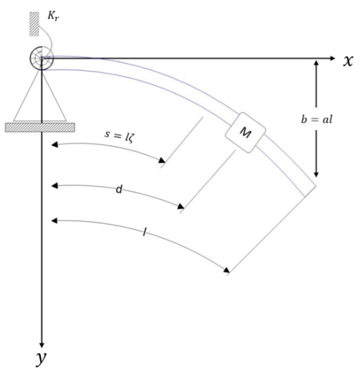
In this section, two different case studies of vibrating beams are thoroughly investigated. A schematic of a uniform beam carrying a lumped mass along its span is depicted in Figure 1. It is considered as case study 1. The length and mass of the beam are l and m, respectively. M is the lumped mass at point the d, ${\mathrm{K}}_{\mathrm{r}}$ represents the rotational stiffness of spring, and s is the arc length of a ${\mathrm{d}}_{\mathrm{s}}$ element.

In order to calculate kinetic and potential energy of beam, the following parameters are applied:

$$\mathsf{\xi }=\frac{\mathrm{s}}{\mathrm{l}},\mathsf{\eta }=\frac{\mathrm{d}}{\mathrm{l}},\mathsf{\mu }=\frac{\mathrm{M}}{\mathrm{ml}}$$

(1)

where $\mathsf{\xi }$ and $\mathsf{\eta }$ represent the span and lumped mass length that non-dimensionalized by the length of the beam. $\mathrm{M}$ represents the mass ratio. Kinetic ($\mathrm{T}$) and potential ($\mathrm{U}$) energies of beam are derived as follows:

$$T=\frac{ml}{2}{{\displaystyle \int }}_0^1\left[1+\mu \delta \left(\xi -\eta \right)\right]\left({\dot{x}}^2+{\dot{y}}^2\right)d\xi ,$$

(2)

and

$$\mathrm{U}=\frac{{\mathrm{EIl}\mathsf{\lambda }}^4}{2}{{\displaystyle \int }}_0^1\left[{{\mathrm{y}}^{″}}^2+{\left(\mathsf{\lambda }{\mathrm{y}}^{\prime }{\mathrm{y}}^{″}\right)}^2+{\mathsf{\lambda }}^4{{\mathrm{y}}^{\prime }}^4{{\mathrm{y}}^{″}}^4\right]\mathrm{d}\mathsf{\xi }.$$

(3)

where $\lambda =1/l$, $\delta \left(\xi -\eta \right)$ is Dirac function, and $\xi$ represents dimensionless arc length. It should be noted that in Equations (2) and (3), the rotary inertia and shear deformation are neglected.

By using the technique of separating variables, the approximate solution is got in the form of $\mathrm{v}\left(\mathrm{t}\right)\mathsf{\varphi }\left(\xi \right)$ where $\mathrm{v}\left(\mathrm{t}\right)$ is an unknown function of time and $\mathsf{\varphi }\left(\xi \right)$ is a normalized eigenfunction of the corresponding linear problem. The superscript dot notation represents differentiation with respect to the time variable. According to the Rayleigh-Ritz procedure with single linear mode, the Lagrangian function is given by:

$$\mathrm{L}=\frac{\mathrm{ml}}{2}\left[{\mathsf{\sigma }}_1{\dot{\mathrm{v}}}^2+{\mathsf{\sigma }}_3{\mathsf{\lambda }}^2{\mathrm{v}}^2{\dot{\mathrm{v}}}^2+{\mathsf{\sigma }}_4{\mathsf{\lambda }}^2{\mathrm{v}}^2{\dot{\mathrm{v}}}^2+{\mathsf{\sigma }}_5{\mathsf{\lambda }}^4{\mathrm{v}}^4{\dot{\mathrm{v}}}^2+{\mathsf{\sigma }}_6{\mathsf{\lambda }}^4{\mathrm{v}}^4{\dot{\mathrm{v}}}^2-\frac{\mathrm{EI}}{\mathrm{m}}{\mathsf{\lambda }}^4\left({\mathsf{\sigma }}_2{\mathrm{v}}^2+{\mathsf{\sigma }}_7{\mathsf{\lambda }}^2{\mathrm{v}}^4+{\mathsf{\sigma }}_8{\mathsf{\lambda }}^4{\mathrm{v}}^4\right)\right]$$

(4)

where ${\sigma }_1$ to ${\sigma }_8$ are following functions:

$$\{\begin{array}{c}{\mathsf{\sigma }}_1={{\displaystyle \int }}_0^1{\mathsf{\varphi }}^2\mathrm{d}\mathsf{\xi }+\mathsf{\mu }{\mathsf{\varphi }}^2\left(\mathsf{\eta }\right),\\ {\mathsf{\sigma }}_2={{\displaystyle \int }}_0^1{{\mathsf{\varphi }}^{″}}^2\mathrm{d}\mathsf{\xi },\\ {\mathsf{\sigma }}_3={{\displaystyle \int }}_0^1{\left({{\displaystyle \int }}_0^{\mathsf{\xi }}{{\mathsf{\varphi }}^{\prime }}^2\mathrm{d}\mathsf{\xi }\right)}^2,\\ {\mathsf{\sigma }}_4=\mu {\left[{\left({{\displaystyle \int }}_0^{\mathsf{\xi }}{{\mathsf{\varphi }}^{\prime }}^2\mathrm{d}\mathsf{\xi }\right)}^2\right]}_{\mathsf{\xi }=\mathsf{\eta }},\end{array}\hspace{1em}\{\begin{array}{c}{\mathsf{\sigma }}_5={{\displaystyle \int }}_0^1\left[\left({{\displaystyle \int }}_0^{\mathsf{\xi }}{{\mathsf{\varphi }}^{\prime }}^2\mathrm{d}\mathsf{\xi }\right)\left({{\displaystyle \int }}_0^{\mathsf{\xi }}{{\mathsf{\varphi }}^{\prime }}^4\mathrm{d}\mathsf{\xi }\right)\right]\mathrm{d}\mathsf{\xi },\\ {\mathsf{\sigma }}_6=\mathsf{\mu }{\left[\left({{\displaystyle \int }}_0^{\mathsf{\xi }}{{\mathsf{\varphi }}^{\prime }}^2\mathrm{d}\mathsf{\xi }\right)\left({{\displaystyle \int }}_0^{\mathsf{\xi }}{{\mathsf{\varphi }}^{\prime }}^4\mathrm{d}\mathsf{\xi }\right)\right]}_{\mathsf{\xi }=\mathsf{\eta }}\\ {\mathsf{\sigma }}_7={{\displaystyle \int }}_0^1{{\mathsf{\varphi }}^{\prime }}^2{\mathsf{\varphi }}^{″}{}^2\mathrm{d}\mathsf{\xi },\\ {\mathsf{\sigma }}_8={{\displaystyle \int }}_0^1{{\mathsf{\varphi }}^{\prime }}^4{\mathsf{\varphi }}^{″}{}^2\mathrm{d}\mathsf{\xi }.\end{array}$$

(5)

By assuming an unextensional beam condition, the length of the neutral axis of the beam will be constant. Therefore, the following constraint relation should apply.

$${\left(1+{\mathsf{\lambda }{\mathrm{x}}^{\prime }}^2\right)}^2+{\mathsf{\lambda }{\mathrm{y}}^{\prime }}^2=1.$$

(6)

The Euler–Lagrange Equation is given by:

$$\frac{\mathrm{d}}{\mathrm{dt}}\left(\frac{\partial \mathrm{L}}{\partial \dot{\mathrm{v}}}\right)-\frac{\partial \mathrm{L}}{\partial \mathrm{v}}=0,$$

(7)

By substituting of Lagrange function (Equation (4)) into Equation (7), the formulation for a restrained uniform beam carrying an intermediate lumped mass is obtained by:

$$\ddot{\mathrm{q}}+\mathsf{\lambda }\mathrm{q}+{\mathsf{\kappa }}_1{\mathrm{q}}^2\ddot{\mathrm{q}}+{\mathsf{\kappa }}_1{\mathrm{q}\dot{\mathrm{q}}}^2+{\mathsf{\kappa }}_2{\mathrm{q}}^4\ddot{\mathrm{q}}+2{\mathsf{\kappa }}_2{\mathrm{q}}^3{\dot{\mathrm{q}}}^2+{\mathsf{\kappa }}_3{\mathrm{q}}^3+{\mathsf{\kappa }}_4{\mathrm{q}}^5=0,$$

(8)

where,

$${\mathsf{\kappa }}_1=\frac{{\mathsf{\sigma }}_3{\mathsf{\sigma }}_4}{{\overline{\mathsf{\Gamma }}}^4{\mathsf{\sigma }}_1},{\mathsf{\kappa }}_2=\frac{{\mathsf{\sigma }}_5{\mathsf{\sigma }}_6}{{\overline{\mathsf{\Gamma }}}^4{\mathsf{\sigma }}_1},{\mathsf{\kappa }}_3=\frac{2{\mathsf{\sigma }}_7}{{\mathsf{\sigma }}_2},{\mathsf{\kappa }}_4=\frac{2{\mathsf{\sigma }}_8}{{\mathsf{\sigma }}_1}$$

(9)

$\overline{\mathsf{\Gamma }}$ in Equation (9) is given by:

$$\overline{\mathsf{\Gamma }}=\sqrt[4]{\frac{\mathrm{m}\overline{\mathsf{\omega }}}{\mathrm{EI}}}\mathrm{l},$$

(10)

where $\overline{\omega }$ is the fundamental frequency of the beam. q in Equation (8) is the dimensionless beam displacement and is equal to $\frac{\overline{\mathsf{\Gamma }}v}{l}$, and dots refer to derivatives according to the new dimensionless time ($\tau =\sqrt{\frac{EI{\lambda }^4}{m}\frac{{\sigma }_1}{{\sigma }_2}}t$). The initial conditions of Equation (8) are chosen as:

$$\mathrm{q}\left(0\right)=\mathrm{A},\dot{\mathrm{q}}\left(0\right)=0$$

(11)

The values of ${\kappa }_1$,${\kappa }_2$,${\kappa }_3$ and ${\kappa }_4$ for three calculation modes are presented in

Table 1. Values of dimensionless rotational stiffness of spring ${\kappa }_i$ in Equation (8) for three modes after [23].

	Mode 1	Mode 2	Mode 3
${\kappa }_1$	0.326845	1.642033	4.051486
${\kappa }_2$	0.129579	0.913055	1.665232
${\kappa }_3$	0.232598	0.313561	0.281418
${\kappa }_4$	0.087584	0.204297	0.149677

.

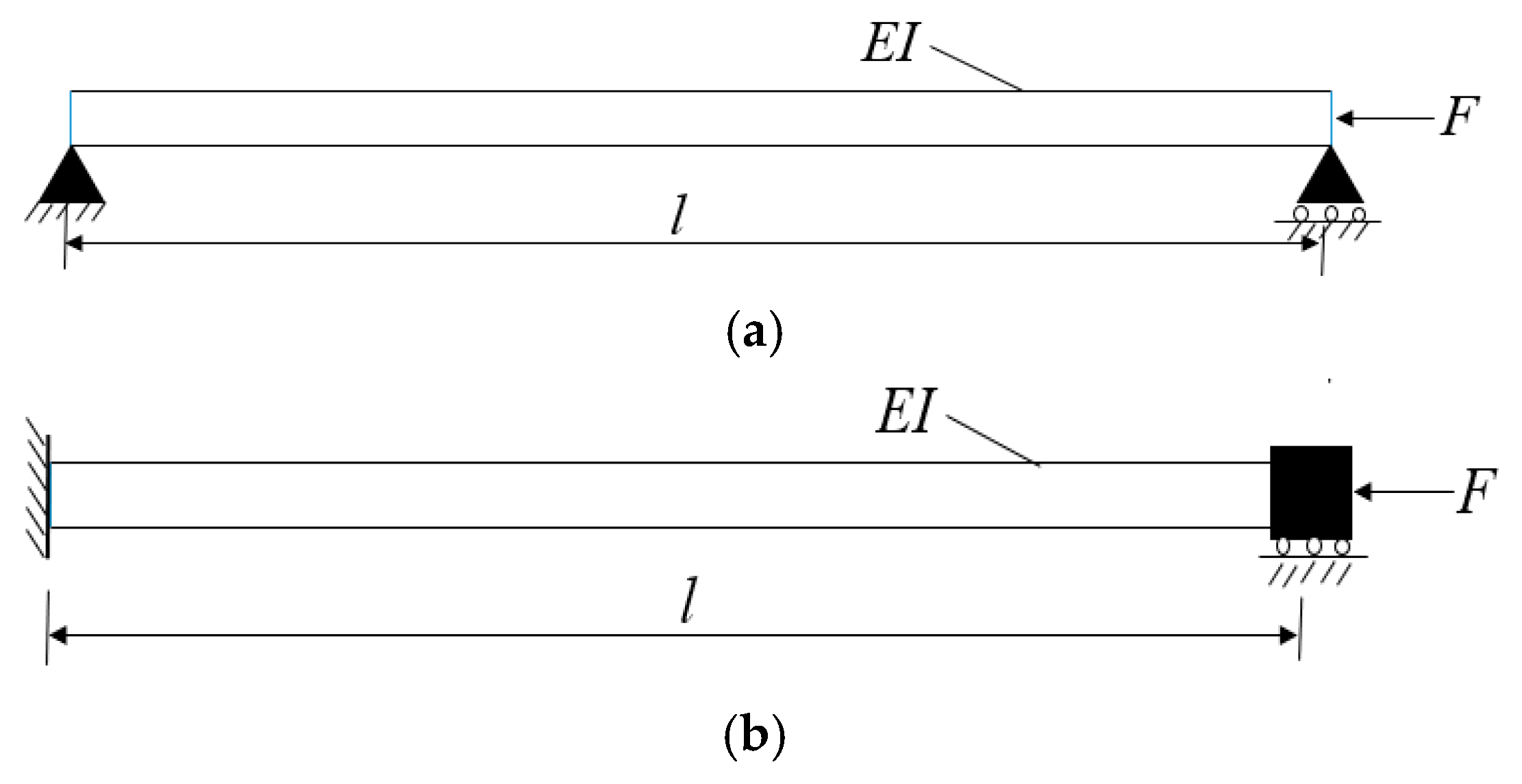
The second case study in this paper is a transversely vibrating quintic nonlinear beam. Figure 2 shows a Euler–Bernoulli beam of length l for two different boundary conditions under force F. Figure 2a is simply supported (S-S) beam and Figure 2b is clamped-clamped (C-C) beam. Typical practical applications of S-S beams with point loadings include bridges, beams in buildings, and beds of machine tools [31]. The C-C beams applies to mechanisms such as mechanical transducer and accelerometers. I is the second moment of inertia, and E represents the modulus of elasticity.

The differential equation in the deformed situation is obtained by:

$$\frac{{\mathrm{d}}^2}{{\mathrm{dx}}^2}\left(\frac{{\mathrm{EIw}}^{″}\left(\mathrm{x},\mathrm{t}\right)}{\sqrt{1+{{\mathrm{w}}^{\prime }}^2{\left(\mathrm{x},\mathrm{t}\right)}^2}}\right)+{\mathrm{Fw}}^{″}\left(\mathrm{x},\mathrm{t}\right)\left[1+\frac{3}{2}{{\mathrm{w}}^{\prime }}^2\left(\mathrm{x},\mathrm{t}\right)\right]+\mathrm{m}\ddot{\mathrm{w}}\left(\mathrm{x},\mathrm{t}\right)=0,$$

(12)

where w is transverse deflection of the beam. The boundary conditions for case (a) and (b) are:

$$\begin{gathered} \mathrm{S}\text{-}\mathrm{S} \mathrm{beam}\mathrm{w}\left(0,\mathrm{t}\right)={\mathrm{w}}^{″}\left(0,\mathrm{t}\right)=0, \\ \mathrm{w}\left(\mathrm{l},\mathrm{t}\right)={\mathrm{w}}^{″}\left(\mathrm{l},\mathrm{t}\right)=0, \end{gathered}$$

(13)

$$\begin{gathered} \mathrm{C}\text{-}\mathrm{C} \mathrm{beam}\mathrm{w}\left(0,\mathrm{t}\right)={\mathrm{w}}^{\prime }\left(0,\mathrm{t}\right)=0, \\ \mathrm{w}\left(\mathrm{l},\mathrm{t}\right)={\mathrm{w}}^{\prime }\left(\mathrm{l},\mathrm{t}\right)=0. \end{gathered}$$

(14)

By assuming the solution of Equation (12) as $\mathrm{w}\left(\mathrm{x},\mathrm{t}\right)=\mathsf{\varphi }\left(\mathrm{x}\right)\overline{\mathrm{q}}\left(\mathrm{t}\right)$ where $\mathsf{\varphi }\left(\mathrm{x}\right)$ is the first eigenmode of the beam vibration. $\mathsf{\varphi }\left(\mathrm{x}\right)$ for S-S beam is given by [30]:

$$\mathsf{\varphi }\left(\mathrm{x}\right)=\sin \left(\frac{\mathsf{\pi }\mathrm{x}}{\mathrm{l}}\right)$$

(15)

and for C-C beam, it is expressed as:

$$\mathsf{\varphi }\left(\mathrm{x}\right)={\left(\frac{\mathrm{x}}{\mathrm{l}}\right)}^2{\left(1-\frac{\mathrm{x}}{\mathrm{l}}\right)}^2.$$

(16)

By applying the Galerkin method, the differential equation in the deformed situation is driven by:

$$\begin{gathered} {{\displaystyle \int }}_0^1\left({\mathrm{EIw}}^4\left[1-\frac{3}{2}{{\mathrm{w}}^{\prime }}^2\left(\mathrm{x},\mathrm{t}\right)+\frac{15}{8}{{\mathrm{w}}^{\prime }}^4\left(\mathrm{x},\mathrm{t}\right)\right]-9\mathrm{EI}{\mathrm{w}}^{\text{‴}}\left(\mathrm{x},\mathrm{t}\right){\mathrm{w}}^{″}\left(\mathrm{x},\mathrm{t}\right){\mathrm{w}}^{\prime }\left(\mathrm{x},\mathrm{t}\right)+\frac{45}{2}{\mathrm{EI}{\mathrm{w}}^{″}}^3\left(\mathrm{x},\mathrm{t}\right){{\mathrm{w}}^{\prime }}^2\left(\mathrm{x},\mathrm{t}\right) \\ +\mathrm{F}{\mathrm{w}}^{″}\left(\mathrm{x},\mathrm{t}\right)\left[1+\frac{3}{2}{{\mathrm{w}}^{\prime }}^2\left(\mathrm{x},\mathrm{t}\right)\right]\mathrm{m}\ddot{\mathrm{w}}\left(\mathrm{x},\mathrm{t}\right)\right)+\mathsf{\varphi }\left(\mathrm{x}\right)\mathrm{dx}=0 \end{gathered}$$

(17)

By introducing $\tau =\sqrt{\frac{EI}{m{l}^4}}$, the non-dimensional nonlinear equation of motion is obtained as follows:

$$\frac{{\mathrm{d}}^2}{{\mathrm{dt}}^2}\mathrm{q}\left(\mathsf{\tau }\right)+\mathrm{aq}\left(\mathsf{\tau }\right)+\mathrm{bq}{\left(\mathsf{\tau }\right)}^3+\mathrm{cq}{\left(\mathsf{\tau }\right)}^5=0$$

(18)

The parameters of Equation (18) for S-S beam are as follow: $a={\pi }^4-\frac{F{l}^2{\pi }^2}{EI}$, $b=-\frac{3}{8}{\pi }^6-\frac{3}{8}\frac{F{l}^2{\pi }^4}{EI}$ and$c=\frac{15}{64}{\pi }^8$. For C-C beam the parameters are $a=500.534-\frac{12.142F{l}^2}{EI}$, $b=-6.654-\frac{0.169F{l}^2}{EI}$ and$c=-0.3673.$ In the next section, the fundamental formulations of AGM will describe.

3. AGM Formulation

The equation of a vibration system can be written as:

$$\mathrm{g}\left(\ddot{\mathrm{x}},\dot{\mathrm{x}},\mathrm{x},{\mathrm{F}}_0\sin \left({\mathsf{\omega }}_0\mathrm{t}\right)\right)=0$$

(19)

${\mathsf{\omega }}_0$ is the angular frequency of the external harmonic force and $F_0$ represents the maximum amplitude of vibration system. The initial conditions are given as:

$$\mathrm{x}\left(0\right)={\mathrm{x}}_0,\dot{\mathrm{x}}\left(0\right)=0$$

(20)

It is worth mentioning that the AGM method can solve vibrating system with and without external forces. Vibration systems without any external forces are presented by the following differential equation:

$$\mathrm{g}\left(\ddot{\mathrm{x}},\dot{\mathrm{x}},\mathrm{x}\right)=0$$

(21)

The general solution of this oscillation system is assumed as:

$$\mathrm{x}\left(\mathrm{t}\right)=\exp \left(-\mathsf{\beta }\mathrm{t}\right)\left\{\mathrm{Acos}\left(\mathsf{\omega }\mathrm{t}\right)+\mathrm{Bsin}\left(\mathsf{\omega }\mathrm{t}\right)\right\}$$

(22)

or alternatively,

$$\mathrm{x}\left(\mathrm{t}\right)=\exp \left(-\mathsf{\beta }\mathrm{t}\right)\mathsf{\alpha }\cos \left(\mathsf{\omega }\mathrm{t}+\mathsf{\phi }\right)$$

(23)

where $\mathsf{\alpha }=\sqrt{{\mathrm{A}}^2+{\mathrm{B}}^2}$ and $\mathsf{\phi }=\arctan \left(\mathrm{B}/\mathrm{A}\right)$. In order to have a more accurate answer, some terms can be added to Equation (23) as:

$$\mathrm{x}\left(\mathrm{t}\right)=\exp \left(-\mathsf{\beta }\mathrm{t}\right)\left\{\mathsf{\alpha }\cos \left(\mathsf{\omega }\mathrm{t}+{\mathsf{\phi }}_1\right)+\mathsf{\gamma }\cos \left(2\mathsf{\omega }\mathrm{t}+{\mathsf{\phi }}_2\right)\right\}$$

(24)

In vibration systems without damping parameters the $\exp \left(-\mathsf{\beta }\mathrm{t}\right)$ term will be deleted from the solution. By applying an external force, ${\mathrm{F}}_0\sin \left({\mathsf{\omega }}_0\mathrm{t}\right),$ on the vibrational systems, the general solution (Equation (19)) will be consisted of two parts. The particular solution (${\mathrm{x}}_{\mathrm{p}}$) and the harmonic solution (${\mathrm{x}}_{\mathrm{h}}$) as follows:

$${\mathrm{x}}_{\mathrm{p}}\left(\mathrm{t}\right)=\mathrm{Rcos}\left({\mathsf{\omega }}_0\mathrm{t}\right)+\mathrm{Qsin}\left({\mathsf{\omega }}_0\mathrm{t}\right)$$

(25)

$${\mathrm{x}}_{\mathrm{h}}\left(\mathrm{t}\right)=\exp \left(-\mathsf{\beta }\mathrm{t}\right)\left\{\mathrm{Acos}\left(\mathsf{\omega }\mathrm{t}\right)+\mathrm{Bsin}\left(2\mathsf{\omega }\mathrm{t}\right)\right\}$$

(26)

By defining $\mathsf{\alpha }=\sqrt{{\mathrm{A}}^2+{\mathrm{B}}^2}$, $\mathsf{\gamma }=\sqrt{{\mathrm{R}}^2+{\mathrm{Q}}^2},$ $\mathsf{\phi }=\arctan \left(\mathrm{B}/\mathrm{A}\right)$, and$\mathsf{\theta }=\arctan \left(\mathrm{Q}/\mathrm{R}\right)$the general solution will yield as:

$$\mathrm{x}\left(\mathrm{t}\right)={\mathrm{x}}_{\mathrm{h}}\left(\mathrm{t}\right)+{\mathrm{x}}_{\mathrm{p}}\left(\mathrm{t}\right)=\exp \left(-\mathsf{\beta }\mathrm{t}\right)\left\{\mathsf{\alpha }\cos \left(\mathsf{\omega }\mathrm{t}+\mathsf{\phi }\right)\right\}+\mathsf{\gamma }\cos \left({\mathsf{\omega }}_0\mathrm{t}+\mathsf{\theta }\right)$$

(27)

The same approach as vibration system without damping, more accurate solution is given by:

$$\mathrm{x}\left(\mathrm{t}\right)=\exp \left(-\mathsf{\beta }\mathrm{t}\right)\left\{\mathsf{\alpha }\cos \left(\mathsf{\omega }\mathrm{t}+{\mathsf{\phi }}_1\right)+\mathsf{\rho }\cos \left(2\mathsf{\omega }\mathrm{t}+{\mathsf{\phi }}_2\right)\right\}+\mathsf{\gamma }\cos \left({\mathsf{\omega }}_0\mathrm{t}+\mathsf{\theta }\right)$$

(28)

In summary the exact general solution for vibrating system is led to:

$$\mathrm{x}\left(\mathrm{t}\right)=\exp \left(-\mathsf{\beta }\mathrm{t}\right)\left\{{\displaystyle \sum }_{\mathrm{k}=1}^{\infty }{\mathsf{\alpha }}_{\mathrm{k}}\cos \left(\mathrm{k}\mathsf{\omega }\mathrm{t}+{\mathsf{\phi }}_{\mathrm{k}}\right)\right\}+\mathsf{\gamma }\cos \left({\mathsf{\omega }}_0\mathrm{t}+\mathsf{\theta }\right)$$

(29)

The unknown parameters in Equation (29) will be computed by applying AGM and using the initial conditions. The $\mathsf{\beta }$ value is zero for a system without damping. Therefore, for a system under vibration Equations (27) and (28) are changed into Equations (30) and (31), respectively:

$$\mathrm{x}\left(\mathrm{t}\right)=\left\{\mathsf{\alpha }\cos \left(\mathsf{\omega }\mathrm{t}+{\mathsf{\phi }}_1\right)+\mathsf{\rho }\cos \left(2\mathsf{\omega }\mathrm{t}+{\mathsf{\phi }}_1\right)\right\}+\mathsf{\gamma }\cos \left({\mathsf{\omega }}_0\mathrm{t}+\mathsf{\theta }\right)$$

(30)

$$\mathrm{x}\left(\mathrm{t}\right)=\left\{{\displaystyle \sum }_{\mathrm{k}=1}^{\infty }{\mathsf{\alpha }}_{\mathrm{k}}\cos \left(\mathrm{k}\mathsf{\omega }\mathrm{t}+{\mathsf{\phi }}_{\mathrm{k}}\right)\right\}+\mathsf{\gamma }\cos \left({\mathsf{\omega }}_0\mathrm{t}+\mathsf{\theta }\right)$$

(31)

In general, the solution of undamped vibrational system in both states (with and without external force) is as follows:

$$\mathrm{x}\left(\mathrm{t}\right)=\mathsf{\alpha }\cos \left(\mathsf{\omega }\mathrm{t}+\mathsf{\phi }\right)+\mathsf{\gamma }\cos \left({\mathsf{\omega }}_0\mathrm{t}+\mathsf{\theta }\right).$$

(32)

In AGM, there are two different approaches to obtain the unknown parameters. The first path is to apply the answer of differential equation to find unknown parameters and the second one is using the main differential equation and its derivatives. In the first method, by considering the initials condition as:

$$\mathrm{x}\left(\mathrm{t}\right)=\mathrm{x}\left(\mathrm{IC}\right),$$

(33)

where IC in Equation (33) is the abbreviation of initial conditions (see Equation (22)), and the unknown parameter will be cleared.

In the second method, the assumed function will be substituted into the solution of the main differential equation instead of its dependent variable (x). The general equation of vibration systems is written by:

$$\mathrm{g}\left(\ddot{\mathrm{x}},\dot{\mathrm{x}},\mathrm{x},{\mathrm{F}}_0\sin \left({\mathsf{\omega }}_0\mathrm{t}\right)\right)=0.$$

(34)

The solution of this vibrational system is considered as:

$$\mathrm{x}=\mathrm{f}\left(\mathrm{t}\right)$$

(35)

By substitute $\mathrm{f}\left(\mathrm{t}\right)$ into Equation (34), the general equation yields as:

$$\mathrm{g}\left(\mathrm{t}\right)=\mathrm{g}\left({\mathrm{f}}^{″}\left(\mathrm{t}\right),{\mathrm{f}}^{\prime }\left(\mathrm{t}\right),\mathrm{f}\left(\mathrm{t}\right),{\mathrm{F}}_0\sin \left({\mathsf{\omega }}_0\mathrm{t}\right)\right)=0$$

(36)

Applying initial conditions on Equation (36) and its derivatives leads to:

$$\{\begin{array}{c}\mathrm{g}\left(\mathrm{IC}\right)=\mathrm{g}\left({\mathrm{f}}^{″}\left(\mathrm{IC}\right),{\mathrm{f}}^{\prime }\left(\mathrm{IC}\right),\mathrm{f}\left(\mathrm{IC}\right),\dots \right)=0,\\ {\mathrm{g}}^{\prime }\left(\mathrm{IC}\right)={\mathrm{g}}^{\prime }\left({\mathrm{f}}^{″}\left(\mathrm{IC}\right),{\mathrm{f}}^{\prime }\left(\mathrm{IC}\right),\mathrm{f}\left(\mathrm{IC}\right),\dots \right)=0,\\ {\mathrm{g}}^{″}\left(\mathrm{IC}\right)={\mathrm{g}}^{″}\left({\mathrm{f}}^{″}\left(\mathrm{IC}\right),{\mathrm{f}}^{\prime }\left(\mathrm{IC}\right),\mathrm{f}\left(\mathrm{IC}\right),\dots \right),=0,\end{array}$$

(37)

According to the initial condition (Equation (20)) and the order of differential equation, n algebraic equations with n unknown parameters will be created and, therefore, constant parameters consist of $\mathsf{\alpha },\mathsf{\beta },\mathsf{\rho },\mathsf{\gamma },$angular frequency $\mathsf{\omega }$, initial phase $\mathsf{\phi },$ and $\mathsf{\theta }$ can be easily computed. Note that in Equation (35), the higher orders of the derivatives of $g\left(t\right)$ can apply until the number of obtained equations is equal to the number of the constant coefficient of the assumed solution. In the next section the proposed AGM will be used to solve the nonlinear transversely vibrating beams with different boundary conditions.

The numerical results in this case RK4 are applied to investigate the accuracy of AGM method. In addition of RK4, the He [23] as the only approach cited in the literature used here to verify the result. The number of arithmetic operations plays an important role in assessing the efficiency of a method. The accuracy and computational effort of He [23] heavily rely on the capability of the approaches and the flexibility of the computer program. For example, the black dashed line in Figure 3a represents the AGM solution with 2 subinterval computations and 650 arithmetic operations, while the blue line denotes the EBM with 124 subinterval integration solution with 53,630 arithmetic operations. The number of arithmetic operations increases exponentially with increasing the number of subintervals and terms.

4. Solution of AGM for Nonlinear Vibrating Beam

This section will describe the details of solution for nonlinear transversely vibrating beams, Equation (8), by AGM. Equation (8) is rewritten as:

$$\mathrm{q}+\mathsf{\lambda }\ddot{\mathrm{q}}+{\mathsf{\kappa }}_1{\mathrm{q}}^2\ddot{\mathrm{q}}+{\mathsf{\kappa }}_1{\mathrm{q}\dot{\mathrm{q}}}^2+{\mathsf{\kappa }}_2{\mathrm{q}}^4\ddot{\mathrm{q}}+2{\mathsf{\kappa }}_2{\mathrm{q}}^3{\dot{\mathrm{q}}}^2+{\mathsf{\kappa }}_3{\mathrm{q}}^3+{\mathsf{\kappa }}_4{\mathrm{q}}^5=0.$$

(38)

The assumed answer of this equation is given by:

$$\mathrm{q}\left(\mathrm{t}\right)=\exp \left(-\mathsf{\beta }\mathrm{t}\right)\left\{\mathsf{\alpha }\cos \left(\mathsf{\omega }\mathrm{t}+{\mathsf{\phi }}_1\right)+\mathsf{\gamma }\cos \left(2\mathsf{\omega }\mathrm{t}+{\mathsf{\phi }}_2\right)\right\}$$

(39)

Since there is no damping component in Equation (37), $\mathsf{\beta }$ is equal to zero and the $\exp \left(-\mathsf{\beta }\mathrm{t}\right)$ term would be removed from Equation (38). Therefore, the assumed solution is:

$$\mathrm{q}\left(\mathrm{t}\right)=\mathsf{\alpha }\cos \left(\mathsf{\omega }\mathrm{t}+{\mathsf{\phi }}_1\right)+\mathsf{\gamma }\cos \left(2\mathsf{\omega }\mathrm{t}+{\mathsf{\phi }}_2\right)$$

(40)

By applying the initial conditions, the constant coefficients and angular frequency ($\mathsf{\omega })$ will be calculated. The initial conditions are applied in two ways. The first direction is to implement the initial conditions into Equation (39) as:

$$\mathrm{q}\left(\mathrm{t}\right)=\mathrm{q}\left(\mathrm{IC}\right).$$

(41)

Thus, the assumed answer leads to:

$$\mathrm{q}\left(0\right)=\mathrm{A}=\mathsf{\alpha }\cos \left({\mathsf{\phi }}_1\right)+\mathsf{\gamma }\cos \left({\mathsf{\phi }}_2\right)$$

(42)

$${\mathrm{q}}^{\prime }\left(0\right)=0=\mathsf{\alpha }\sin \left({\mathsf{\phi }}_1\right)\mathsf{\omega }+\mathsf{\gamma }\sin \left({\mathsf{\phi }}_2\right)\mathsf{\omega }.$$

(43)

The third equation will generate by applying the initial condition on the main differential equation which in this case is Equation (38) and its derivatives as follow:

$$\mathrm{g}\left({\mathrm{q}}^{\prime }\left(\mathrm{IC}\right)\right)={\mathrm{g}}^{\prime }\left({\mathrm{q}}^{\prime }\left(\mathrm{IC}\right)\right)=0$$

(44)

This leads to obtain the following equations.

$$\begin{gathered} \mathrm{g}\left(\mathrm{q}\left(0\right)\right): \mathsf{\alpha }\cos \left({\mathsf{\varphi }}_1\right){\mathsf{\omega }}^2+4\gamma \cos \left({\mathsf{\varphi }}_2\right){\mathsf{\omega }}^2-\mathsf{\lambda }\left(\mathsf{\alpha }\cos \left({\mathsf{\varphi }}_1\right)+\gamma \cos \left({\mathsf{\varphi }}_2\right)\right) \\ -{\mathsf{\epsilon }}_1{\left(\mathsf{\alpha }\cos \left({\mathsf{\varphi }}_1\right)+\mathsf{\gamma }\cos \left({\mathsf{\varphi }}_2\right)\right)}^2\left(-\mathsf{\alpha }\cos \left({\mathsf{\varphi }}_1\right){\mathsf{\omega }}^2-4\mathsf{\gamma }\cos \left({\mathsf{\varphi }}_2\right){\mathsf{\omega }}^2\right) \\ -{\mathsf{\epsilon }}_1\left(\mathsf{\alpha }\cos \left({\mathsf{\varphi }}_1\right)+\mathsf{\gamma }\cos \left({\mathsf{\varphi }}_2\right)\right){\left(-\mathsf{\alpha }\sin \left({\mathsf{\varphi }}_1\right)\mathsf{\omega }-2\mathsf{\gamma }\sin \left({\mathsf{\varphi }}_2\right)\mathsf{\omega }\right)}^2 \\ -{\mathsf{\epsilon }}_2{\left(\mathsf{\alpha }\cos \left({\mathsf{\varphi }}_1\right)+\mathsf{\gamma }\cos \left({\mathsf{\varphi }}_2\right)\right)}^4\left(-\mathsf{\alpha }\cos \left({\mathsf{\varphi }}_1\right){\mathsf{\omega }}^2-4\mathsf{\gamma }\cos \left({\mathsf{\varphi }}_2\right){\mathsf{\omega }}^2\right) \\ -2{\mathsf{\epsilon }}_2{\left(\mathsf{\alpha }\cos \left({\mathsf{\varphi }}_1\right)+\mathsf{\gamma }\cos \left({\mathsf{\varphi }}_2\right)\right)}^3{\left(-\mathsf{\alpha }\sin \left({\mathsf{\varphi }}_1\right)\mathsf{\omega }-2\mathsf{\gamma }\cos \left({\mathsf{\varphi }}_2\right)\mathsf{\omega }\right)}^2 \\ -{\mathsf{\epsilon }}_3{\left(\mathsf{\alpha }\sin \left({\mathsf{\varphi }}_1\right)+\mathsf{\gamma }\cos \left({\mathsf{\varphi }}_2\right)\right)}^3-{\mathsf{\epsilon }}_4{\left(\mathsf{\alpha }\sin \left({\mathsf{\varphi }}_1\right)+\mathsf{\gamma }\cos \left({\mathsf{\varphi }}_2\right)\right)}^5=0, \end{gathered}$$

(45)

$$\begin{gathered} {\mathrm{g}}^{\prime }\left(\mathrm{q}\left(0\right)\right):-\mathsf{\alpha }\sin \left({\mathsf{\varphi }}_1\right){\mathsf{\omega }}^3-8\mathsf{\gamma }\cos \left({\mathsf{\varphi }}_2\right){\mathsf{\omega }}^3 \\ -\mathsf{\lambda }\left(\mathsf{\alpha }\sin \left({\mathsf{\varphi }}_1\right)\mathsf{\omega }-2\mathsf{\gamma }\sin \left({\mathsf{\varphi }}_2\right)\mathsf{\omega }\right) \\ -4{\mathsf{\epsilon }}_1\left(\mathsf{\alpha }\cos \left({\mathsf{\varphi }}_1\right)+\mathsf{\gamma }\cos \left({\mathsf{\varphi }}_2\right)\right)\left(-\mathsf{\alpha }\cos \left({\mathsf{\varphi }}_1\right){\mathsf{\omega }}^2-4\mathsf{\gamma }\cos \left({\mathsf{\varphi }}_2\right){\mathsf{\omega }}^2\right) \\ \left(-\mathsf{\alpha }\sin \left({\mathsf{\varphi }}_1\right)\mathsf{\omega }-2\mathsf{\gamma }\sin \left({\mathsf{\varphi }}_2\right)\mathsf{\omega }\right)-{\mathsf{\epsilon }}_1{\left(\mathsf{\alpha }\cos \left({\mathsf{\varphi }}_1\right)\mathsf{\omega }+\mathsf{\gamma }\cos \left({\mathsf{\varphi }}_2\right)\right)}^2 \\ \left(\mathsf{\alpha }\sin \left({\mathsf{\varphi }}_1\right){\mathsf{\omega }}^3+8\mathsf{\gamma }\sin \left({\mathsf{\varphi }}_2\right){\mathsf{\omega }}^3\right)-{\mathsf{\epsilon }}_1{\left(-\mathsf{\alpha }\sin \left({\mathsf{\varphi }}_1\right)\mathsf{\omega }-2\mathsf{\gamma }\cos \left({\mathsf{\varphi }}_2\right)\mathsf{\omega }\right)}^3 \\ -8{\mathsf{\epsilon }}_2{\left(\mathsf{\alpha }\cos \left({\mathsf{\varphi }}_1\right)+\mathsf{\gamma }\cos \left({\mathsf{\varphi }}_2\right)\right)}^3\left(-\mathsf{\alpha }\cos \left({\mathsf{\varphi }}_1\right){\mathsf{\omega }}^2-4\mathsf{\gamma }\cos \left({\mathsf{\varphi }}_2\right){\mathsf{\omega }}^2\right) \\ \left(-\mathsf{\alpha }\sin \left({\mathsf{\varphi }}_1\right)\mathsf{\omega }-2\mathsf{\gamma }\sin \left({\mathsf{\varphi }}_2\right)\mathsf{\omega }\right)-{\mathsf{\epsilon }}_2{\left(\mathsf{\alpha }\cos \left({\mathsf{\varphi }}_1\right)\mathsf{\omega }+\mathsf{\gamma }\cos \left({\mathsf{\varphi }}_2\right)\mathsf{\omega }\right)}^4 \\ \left(\mathsf{\alpha }\sin \left({\mathsf{\varphi }}_1\right){\mathsf{\omega }}^3+8\mathsf{\gamma }\sin \left({\mathsf{\varphi }}_2\right){\mathsf{\omega }}^3\right)-6{\mathsf{\epsilon }}_2{\left(\mathsf{\alpha }\cos \left({\mathsf{\varphi }}_1\right)+\mathsf{\gamma }\cos \left({\mathsf{\varphi }}_2\right)\right)}^2 \\ {\left(-\mathsf{\alpha }\sin \left({\mathsf{\varphi }}_1\right)\mathsf{\omega }-2\mathsf{\gamma }\sin \left({\mathsf{\varphi }}_2\right)\mathsf{\omega }\right)}^3-3{\mathsf{\epsilon }}_3{\left(\mathsf{\alpha }\cos \left({\mathsf{\varphi }}_1\right)+\mathsf{\gamma }\cos \left({\mathsf{\varphi }}_2\right)\right)}^2 \\ \left(-\mathsf{\alpha }\sin \left({\mathsf{\varphi }}_1\right)\mathsf{\omega }-2\mathsf{\gamma }\sin \left({\mathsf{\varphi }}_2\right)\mathsf{\omega }\right)-5{\mathsf{\epsilon }}_4{\left(\mathsf{\alpha }\cos \left({\mathsf{\varphi }}_1\right)+\mathsf{\gamma }\cos \left({\mathsf{\varphi }}_2\right)\right)}^4 \\ \left(-\mathsf{\alpha }\sin \left({\mathsf{\varphi }}_1\right)\mathsf{\omega }-2\mathsf{\gamma }\sin \left({\mathsf{\varphi }}_2\right)\mathsf{\omega }\right)=0, \end{gathered}$$

(46)

$$\begin{gathered} {\mathrm{g}}^{″}\left(\mathrm{q}\left(0\right)\right):-\mathsf{\alpha }\cos \left({\mathsf{\varphi }}_1\right){\mathsf{\omega }}^4-16\mathsf{\gamma }\cos \left({\mathsf{\varphi }}_2\right){\mathsf{\omega }}^4 \\ -\mathsf{\lambda }\left(\mathsf{\alpha }\cos \left({\mathsf{\varphi }}_1\right){\mathsf{\omega }}^2+2\mathsf{\gamma }\cos \left({\mathsf{\varphi }}_2\right){\mathsf{\omega }}^2\right)-7{\mathsf{\epsilon }}_1{\left(-\mathsf{\alpha }\sin \left({\mathsf{\varphi }}_1\right)\mathsf{\omega }-2\mathsf{\gamma }\sin \left({\mathsf{\varphi }}_2\right)\mathsf{\omega }\right)}^2 \\ \left(-\mathsf{\alpha }\cos \left({\mathsf{\varphi }}_1\right){\mathsf{\omega }}^2-4\mathsf{\gamma }\cos \left({\mathsf{\varphi }}_2\right){\mathsf{\omega }}^2\right)-6{\mathsf{\epsilon }}_1\left(\mathsf{\alpha }\cos \left({\mathsf{\varphi }}_1\right)+\mathsf{\gamma }\cos \left({\mathsf{\varphi }}_2\right)\right) \\ \left(\mathsf{\alpha }\sin \left({\mathsf{\varphi }}_1\right){\mathsf{\omega }}^3+8\mathsf{\gamma }\cos \left({\mathsf{\varphi }}_2\right){\mathsf{\omega }}^3\right)\left(-\mathsf{\alpha }\sin \left({\mathsf{\varphi }}_1\right)\mathsf{\omega }-2\mathsf{\gamma }\sin \left({\mathsf{\varphi }}_2\right)\mathsf{\omega }\right) \\ -4{\mathsf{\epsilon }}_1\left(\mathsf{\alpha }\cos \left({\mathsf{\varphi }}_1\right)+\mathsf{\gamma }\cos \left({\mathsf{\varphi }}_2\right)\right){\left(-\mathsf{\alpha }\cos \left({\mathsf{\varphi }}_1\right){\mathsf{\omega }}^2-4\mathsf{\gamma }\cos \left({\mathsf{\varphi }}_2\right){\mathsf{\omega }}^2\right)}^2 \\ -{\mathsf{\epsilon }}_1{\left(\mathsf{\alpha }\cos \left({\mathsf{\varphi }}_1\right)+\mathsf{\gamma }\cos \left({\mathsf{\varphi }}_2\right)\right)}^2\left(\mathsf{\alpha }\cos \left({\mathsf{\varphi }}_1\right){\mathsf{\omega }}^4+16\mathsf{\gamma }\cos \left({\mathsf{\varphi }}_2\right){\mathsf{\omega }}^4\right) \\ -42{\mathsf{\epsilon }}_2{\left(\mathsf{\alpha }\cos \left({\mathsf{\varphi }}_1\right)+16\mathsf{\gamma }\cos \left({\mathsf{\varphi }}_2\right)\right)}^2\left(-\mathsf{\alpha }\cos \left({\mathsf{\varphi }}_1\right){\mathsf{\omega }}^2-4\mathsf{\gamma }\cos \left({\mathsf{\varphi }}_2\right){\mathsf{\omega }}^2\right) \\ {\left(-\mathsf{\alpha }\sin \left({\mathsf{\varphi }}_1\right)\mathsf{\omega }-2\mathsf{\gamma }\sin \left({\mathsf{\varphi }}_2\right)\mathsf{\omega }\right)}^2-12{\mathsf{\epsilon }}_2{\left(\mathsf{\alpha }\cos \left({\mathsf{\varphi }}_1\right)+\mathsf{\gamma }\cos \left({\mathsf{\varphi }}_2\right)\right)}^3 \\ \left(\mathsf{\alpha }\sin \left({\mathsf{\varphi }}_1\right){\mathsf{\omega }}^3+8\mathsf{\gamma }\sin \left({\mathsf{\varphi }}_2\right){\mathsf{\omega }}^3\right)\left(-\mathsf{\alpha }\sin \left({\mathsf{\varphi }}_1\right)\mathsf{\omega }-2\mathsf{\gamma }\sin \left({\mathsf{\varphi }}_2\right)\mathsf{\omega }\right) \\ -8{\mathsf{\epsilon }}_2{\left(\mathsf{\alpha }\cos \left({\mathsf{\varphi }}_1\right)-\mathsf{\gamma }\cos \left({\mathsf{\varphi }}_2\right)\right)}^3{\left(-\mathsf{\alpha }\cos \left({\mathsf{\varphi }}_1\right){\mathsf{\omega }}^2-4\mathsf{\gamma }\cos \left({\mathsf{\varphi }}_2\right){\mathsf{\omega }}^2\right)}^2 \\ -{\mathsf{\epsilon }}_2{\left(\mathsf{\alpha }\cos \left({\mathsf{\varphi }}_1\right)+\mathsf{\gamma }\cos \left({\mathsf{\varphi }}_2\right)\right)}^4\left(\mathsf{\alpha }\cos \left({\mathsf{\varphi }}_1\right){\mathsf{\omega }}^4+16\mathsf{\gamma }\cos \left({\mathsf{\varphi }}_2\right){\mathsf{\omega }}^4\right) \\ -12{\mathsf{\epsilon }}_2\left(\mathsf{\alpha }\cos \left({\mathsf{\varphi }}_1\right)+\mathsf{\gamma }\cos \left({\mathsf{\varphi }}_2\right)\right){\left(-\mathsf{\alpha }\sin \left({\mathsf{\varphi }}_1\right)\mathsf{\omega }-2\mathsf{\gamma }\sin \left({\mathsf{\varphi }}_2\right)\mathsf{\omega }\right)}^4 \\ -6{\mathsf{\epsilon }}_3\left(\mathsf{\alpha }\cos \left({\mathsf{\varphi }}_1\right)+\mathsf{\gamma }\cos \left({\mathsf{\varphi }}_2\right)\right){\left(-\mathsf{\alpha }\sin \left({\mathsf{\varphi }}_1\right)\mathsf{\omega }-2\mathsf{\gamma }\sin \left({\mathsf{\varphi }}_2\right)\mathsf{\omega }\right)}^2 \\ -3{\mathsf{\epsilon }}_3{\left(\mathsf{\alpha }\cos \left({\mathsf{\varphi }}_1\right)+\mathsf{\gamma }\cos \left({\mathsf{\varphi }}_2\right)\right)}^2\left(-\mathsf{\alpha }\cos \left({\mathsf{\varphi }}_1\right){\mathsf{\omega }}^2-4\mathsf{\gamma }\cos \left({\mathsf{\varphi }}_2\right){\mathsf{\omega }}^2\right) \\ -20{\mathsf{\epsilon }}_4{\left(\mathsf{\alpha }\cos \left({\mathsf{\varphi }}_1\right)+\mathsf{\gamma }\cos \left({\mathsf{\varphi }}_2\right)\right)}^3{\left(-\mathsf{\alpha }\sin \left({\mathsf{\varphi }}_1\right)\mathsf{\omega }-2\mathsf{\gamma }\sin \left({\mathsf{\varphi }}_2\right)\mathsf{\omega }\right)}^2 \\ -5{\mathsf{\epsilon }}_4{\left(\mathsf{\alpha }\cos \left({\mathsf{\varphi }}_1\right)+\mathsf{\gamma }\cos \left({\mathsf{\varphi }}_2\right)\right)}^4\left(-\mathsf{\alpha }\cos \left({\mathsf{\varphi }}_1\right){\mathsf{\omega }}^2-4\mathsf{\gamma }\cos \left({\mathsf{\varphi }}_2\right){\mathsf{\omega }}^2\right), \end{gathered}$$

(47)

To sum up, there are five algebraic Equations (41)–(46) and five unknown parameters consisting of $\alpha ,\mathsf{\gamma },{\varphi }_1,{\varphi }_2$ and $\omega .$ Therefore, these parameters can easily be computed.

This procedure is also applied for transversely vibrating quintic nonlinear beam (Equation (18)). According to Equation (43), $g\left(q\left(0\right)\right)$, $g^{\prime }\left(q\left(0\right)\right)$, and $g^{″}\left(q\left(0\right)\right)$ are given by:

$$\begin{gathered} \mathrm{g}\left(\mathrm{q}\left(0\right)\right):\mathsf{\alpha }\cos \left({\mathsf{\varphi }}_1\right){\mathsf{\omega }}^2+4\mathsf{\gamma }\cos \left({\mathsf{\varphi }}_2\right){\mathsf{\omega }}^2-\mathrm{a}\mathsf{\alpha }\cos \left({\mathsf{\varphi }}_1\right)+\mathsf{\gamma }\cos \left({\mathsf{\varphi }}_2\right) \\ -\mathrm{b}{\left(\mathsf{\alpha }\cos \left({\mathsf{\varphi }}_1\right)+\mathsf{\gamma }\cos \left({\mathsf{\varphi }}_2\right)\right)}^3-\mathrm{c}{\left(\mathsf{\alpha }\cos \left({\mathsf{\varphi }}_1\right)-\mathsf{\gamma }\cos \left({\mathsf{\varphi }}_2\right)\right)}^5=0, \end{gathered}$$

(48)

$$\begin{gathered} {\mathrm{g}}^{\prime }\left(\mathrm{q}\left(0\right)\right):-\mathsf{\alpha }\sin \left({\mathsf{\varphi }}_1\right){\mathsf{\omega }}^3-8\mathsf{\gamma }\cos \left({\mathsf{\varphi }}_2\right){\mathsf{\omega }}^3+\mathrm{a}\mathsf{\alpha }\sin \left({\mathsf{\varphi }}_1\right)\mathsf{\omega }+2\mathsf{\gamma }\sin \left({\mathsf{\varphi }}_2\right)\mathsf{\omega } \\ +3\mathrm{b}{\left(\mathsf{\alpha }\cos \left({\mathsf{\varphi }}_1\right)+\mathsf{\gamma }\cos \left({\mathsf{\varphi }}_2\right)\right)}^2\left(-\mathsf{\alpha }\sin \left({\mathsf{\varphi }}_1\right)\mathsf{\omega }-2\mathsf{\gamma }\sin \left({\mathsf{\varphi }}_2\right)\mathsf{\omega }\right) \\ -5\mathrm{c}{\left(\mathsf{\alpha }\cos \left({\mathsf{\varphi }}_1\right)+\mathsf{\gamma }\cos \left({\mathsf{\varphi }}_2\right)\right)}^4\left(-\mathsf{\alpha }\sin \left({\mathsf{\varphi }}_1\right)\mathsf{\omega }-2\mathsf{\gamma }\sin \left({\mathsf{\varphi }}_2\right)\mathsf{\omega }\right)=0, \end{gathered}$$

(49)

$$\begin{gathered} {\mathrm{g}}^{″}\left(\mathrm{q}\left(0\right)\right):-\mathsf{\alpha }\cos \left({\mathsf{\varphi }}_1\right){\mathsf{\omega }}^4-16\mathsf{\gamma }\cos \left({\mathsf{\varphi }}_2\right){\mathsf{\omega }}^4 \\ -\mathrm{a}\left(-\mathsf{\alpha }\cos \left({\mathsf{\varphi }}_1\right){\mathsf{\omega }}^2-4\mathsf{\gamma }\cos \left({\mathsf{\varphi }}_2\right){\mathsf{\omega }}^2\right)-6\mathrm{b}\left(\mathsf{\alpha }\cos \left({\mathsf{\varphi }}_1\right)+\mathsf{\gamma }\cos \left({\mathsf{\varphi }}_2\right)\right) \\ {\left(-\mathsf{\alpha }\sin \left({\mathsf{\varphi }}_1\right)\mathsf{\omega }-2\mathsf{\gamma }\sin \left({\mathsf{\varphi }}_2\right)\mathsf{\omega }\right)}^2-3\mathrm{b}{\left(\mathsf{\alpha }\cos \left({\mathsf{\varphi }}_1\right)+\mathsf{\gamma }\cos \left({\mathsf{\varphi }}_2\right)\right)}^2 \\ {\left(-\mathsf{\alpha }\cos \left({\mathsf{\varphi }}_1\right){\mathsf{\omega }}^2-4\mathsf{\gamma }\cos \left({\mathsf{\varphi }}_2\right){\mathsf{\omega }}^2\right)}^2-20\mathrm{c}{\left(\mathsf{\alpha }\cos \left({\mathsf{\varphi }}_1\right)+16\mathsf{\gamma }\cos \left({\mathsf{\varphi }}_2\right)\right)}^3 \\ {\left(-\mathsf{\alpha }\sin \left({\mathsf{\varphi }}_1\right)\mathsf{\omega }-2\mathsf{\gamma }\sin \left({\mathsf{\varphi }}_2\right)\mathsf{\omega }\right)}^2-5\mathrm{c}{\left(\mathsf{\alpha }\cos \left({\mathsf{\varphi }}_1\right)+\mathsf{\gamma }\cos \left({\mathsf{\varphi }}_2\right)\right)}^4 \\ {\left(-\mathsf{\alpha }\cos \left({\mathsf{\varphi }}_1\right){\mathsf{\omega }}^2-4\mathsf{\gamma }\cos \left({\mathsf{\varphi }}_2\right){\mathsf{\omega }}^2\right)}^2-0.129579{\left(\mathsf{\alpha }\cos \left({\mathsf{\varphi }}_1\right)+\mathsf{\gamma }\cos \left({\mathsf{\varphi }}_2\right)\right)}^4 \\ \left(\mathsf{\alpha }\cos \left({\mathsf{\varphi }}_1\right){\mathsf{\omega }}^2-4\mathsf{\gamma }\cos \left({\mathsf{\varphi }}_2\right){\mathsf{\omega }}^2\right)=0. \end{gathered}$$

(50)

By solving the set of Equations (41)–(42) and (47)–(49) together, the five unknown parameters $\alpha ,\mathsf{\gamma },{\varphi }_1,{\varphi }_2$ and $\omega$ will computed for a transversely vibrating quintic nonlinear beam (Equation (18)). In the next section, to illustrate the applicability and accuracy of the AGM method, various case studies of transversely vibrating quintic nonlinear beam will investigate.

4.1. Uniform Beam Carrying a Lumped Mass

Equation (8) represents the dimensionless unimodal temporal formulation for a uniform beam carrying a lumped mass. By considering of $\lambda =0.5$, A = 0.5, ${\kappa }_1=0.326845$,${\kappa }_2=0.129579$, ${\kappa }_3=0.232598,$ and ${\kappa }_4=0.087584$, and solving the set of Equations (41)–(46), the unknown parameters of assumed solution for Equation (8) are computed as:

$$\mathsf{\alpha }=0.5058380464,\gamma =-0.005838046389,{\mathsf{\varphi }}_1=6.283185307,{\mathsf{\varphi }}_2=6.283185307\mathrm{and}\mathsf{\omega }=-0.7320856112.$$

(51)

Therefore, the general solution of Equation (8) is given by:

$$\mathrm{q}\left(\mathrm{t}\right)=0.5058380464\cos \left(0.7320856112\mathrm{t}+6.283185307\right)-0.005838046389\cos \left(1.464171222\mathrm{t}-6.283185307\right)$$

(52)

The following solution belongs to modes 2 with A = 0.1 and$\lambda =0.2$

$$\mathrm{q}\left(\mathrm{t}\right)=0.1003687765\cos \left(0.4495463167\mathrm{t}-3.141592654\right)-0.0003687764765\cos \left(0.8990926334\mathrm{t}\right),$$

(53)

The response of mode 3 with A = 0.01 and $\lambda =0.3$ is presented in Equation (53).

$$\mathrm{q}\left(\mathrm{t}\right)=-0.00002549837711\cos \left(0.2735572113\mathrm{t}\right)-0.01002549838\cos \left(0.5471144226\mathrm{t}\right).$$

(54)

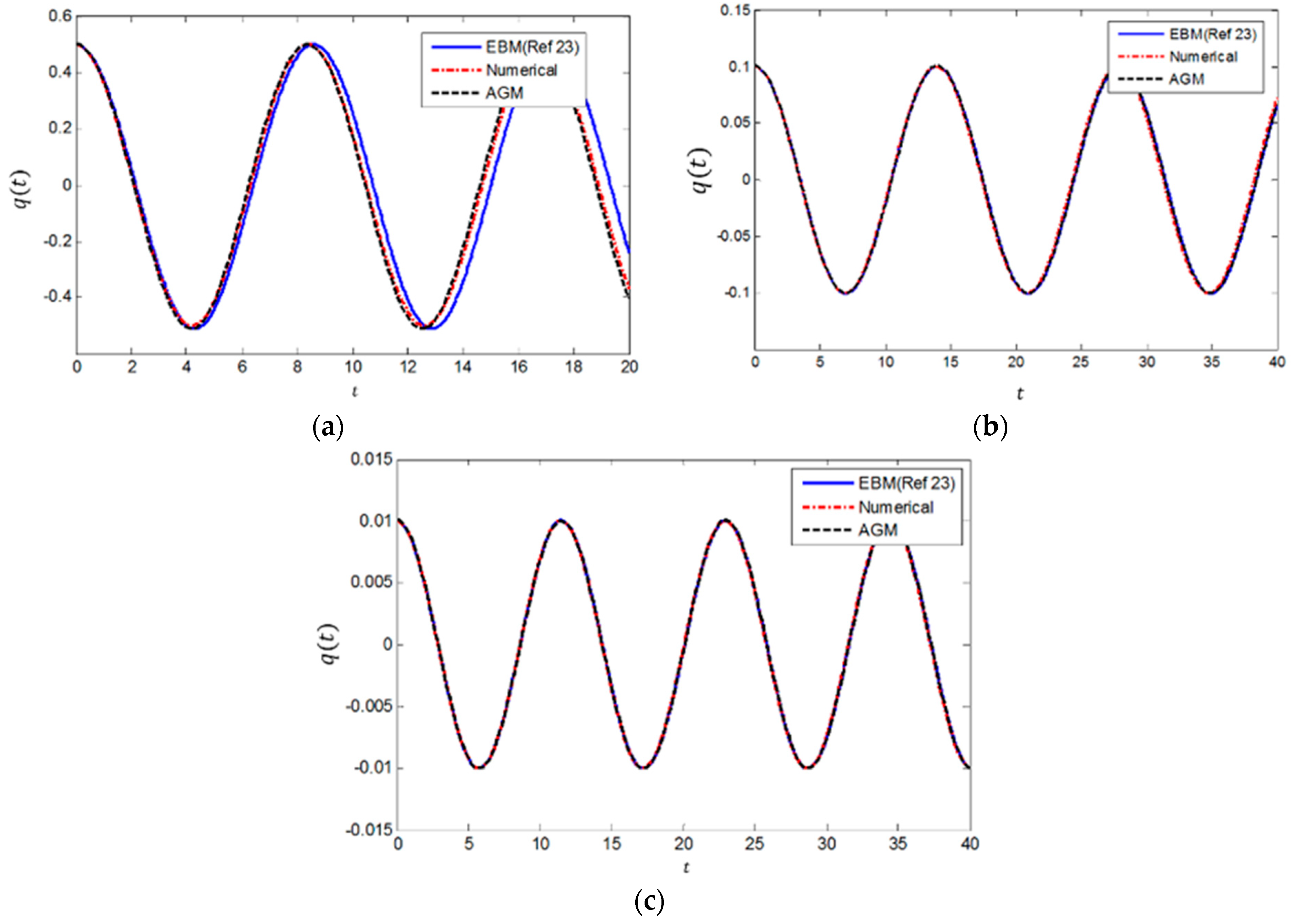
Figure 3 shows the results obtained by AGM for uniform beam carrying a lumped mass. In order to check the preciseness of the presented method, AGM is compared with EBM and the numerical method. It is obvious that the AGM method has a good efficiency to solve uniform beam carrying lumped mass under three mode conditions. The black dashed line in Figure 3a represents the AGM solution with 2 subinterval computations and 650 arithmetic operations, while the blue line denotes the EBM with 124 subinterval integration solution with 53,630 arithmetic operations. The number of arithmetic operations increases exponentially with an increasing the number of subintervals and terms.

To further check of AGM accuracy in

Table 2. Comparison between AGM, EBM and exact numerical solution for mode 1 in Table 1 (λ = 0.2).

A	${\mathit{\omega }}_{\mathit{A}\mathit{G}\mathit{M}}$	${\mathit{\omega }}_{\mathit{E}\mathit{B}\mathit{M}}$ [20]	${\mathit{\omega }}_{\mathit{N}}$ [20]
0.01	0.4472	0.4472	0.4472
0.05	0.4475	0.4476	0.4479
0.1	0.4483	0.4491	0.4490
0.5	0.4769	0.4923	0.4921
1	0.6017	0.6215	0.6211

and

Table 3. Comparison between AGM, EBM and exact numerical solution for mode 1 in Table 1 (λ = 0.5).

A	${\mathit{\omega }}_{\mathit{A}\mathit{G}\mathit{M}}$	${\mathit{\omega }}_{\mathit{E}\mathit{B}\mathit{M}}$ [23]	${\mathit{\omega }}_{\mathit{N}}$ [23]
0.01	0.7071	0.7071	0.7071
0.05	0.7073	0.7076	0.7075
0.1	0.7080	0.7084	0.7082
0.5	0.7322	0.7336	0.7333
1	0.8108	0.8116	0.8115

the frequency solutions are compared with a numerical method and EBM [23,28]. The presentation here is limited into initial parameters and solutions of frequency modes 1–3 used in [23,28]. It is worth to note the applicability of AGM is further checked in other ranges of frequencies and yield a good agreement.

4.2. Transversely Vibrating Quintic Nonlinear Beam

The non-dimensional nonlinear equation of motion for transversely vibrating quintic nonlinear beam is given by:

$$\frac{{\mathrm{d}}^2}{{\mathrm{dt}}^2}\mathrm{q}\left(\mathsf{\tau }\right)+\mathrm{aq}\left(\mathsf{\tau }\right)+\mathrm{bq}{\left(\mathsf{\tau }\right)}^3+\mathrm{cq}{\left(\mathsf{\tau }\right)}^5=0$$

(55)

Three examples with different coefficient values are selected to be solved in this section. Case study 1 represents a C-C beam with constant parameters of $a=379.1140, b=-8.3480,c=-0.3673$ and $\frac{p{l}^2}{EI}=10$. Figure 4 shows the obtained results of C-C beam with proposed parameters by AGM, EBM and the numerical method. This figure confirms the efficiency of AGM for this case study.

Table 4. Comparison between AGM, EBM and exact numerical solution (C-C beam).

A	${\mathit{\omega }}_{\mathit{A}\mathit{G}\mathit{M}}$	${\mathit{\omega }}_{\mathit{E}\mathit{B}\mathit{M}}$ [23]	${\mathit{\omega }}_{\mathit{N}}$ [23]
0.1	19.4692	19.4692	19.4692
0.3	19.4562	19.4563	19.4563
0.5	19.4305	19.4303	19.4302
1	19.3040	19.3039	19.2936

compares the natural frequencies obtained by these three methods for various values of amplitude.

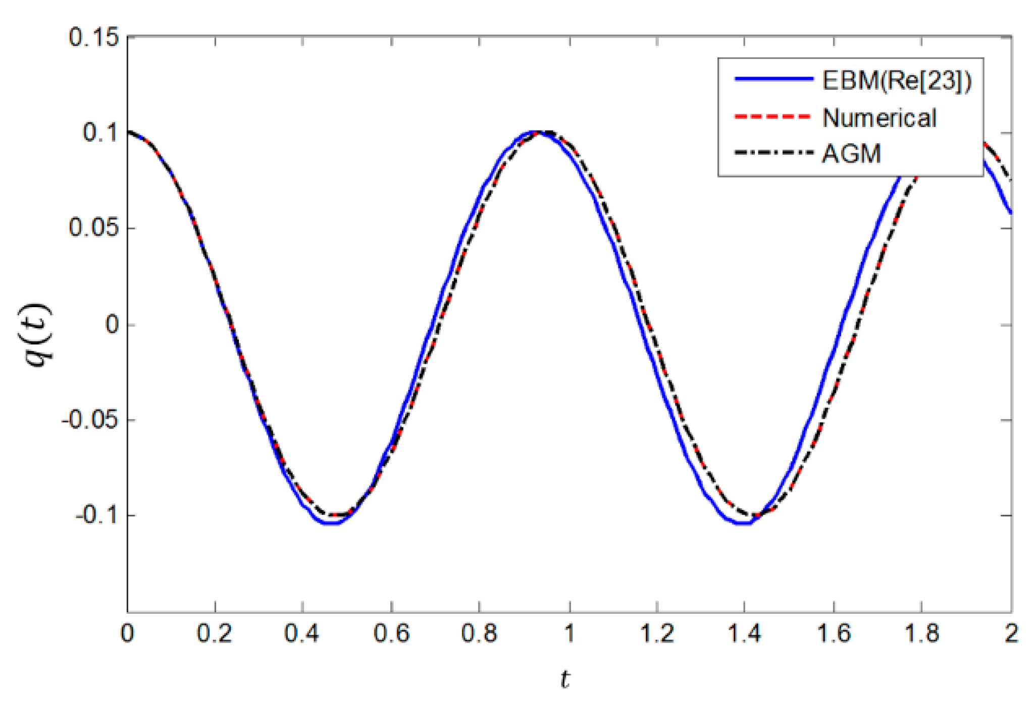
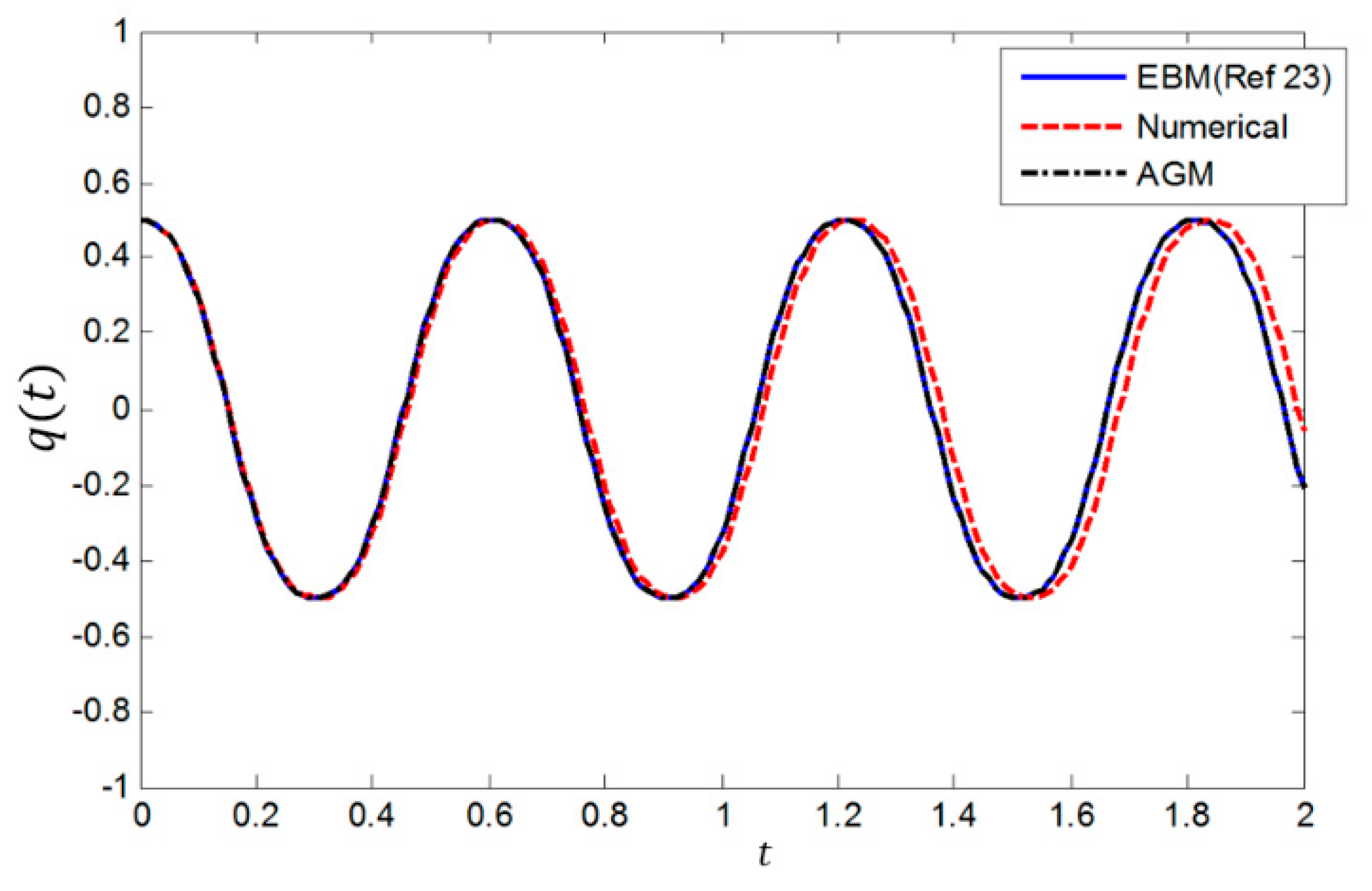
A simply supported S-S beam is selected for case study 2 where$\mathrm{a}=48.0611,\mathrm{b}=-543.1630,\mathrm{c}=-2223.874$, and $\frac{{\mathrm{pl}}^2}{\mathrm{EI}}=5$. Figure 5 displays the obtained solution of this case with AGM, EBM, and numerical method. AGM results has very satisfactory pattern compared with other two methods.

Table 5. Comparison between AGM, EBM, and exact numerical solution (S-S beam).

A	${\mathit{\omega }}_{\mathit{A}\mathit{G}\mathit{M}}$	${\mathit{\omega }}_{\mathit{e}\mathit{b}\mathit{m}}$ [23]	${\mathit{\omega }}_{\mathit{N}}$ [23]
0.1	6.7741	6.6421	6.6417
0.3	4.8036	4.6803	4.6792
0.5	5.1944	5.2246	5.5985
1	30.7202	30.6259	30.4103

compares the natural frequencies obtained by these three methods for various values of amplitude. And finally, Figure 6 shows the results of case study 3 for a simply supported S-S beam where $a=48.0611, b=-543.1630,c=2223.874$, and $\frac{p{l}^2}{EI}=5$.

Table 6. Comparison between AGM, EBM and exact numerical solution for S-S beam (case study 3).

A	${\mathit{\omega }}_{\mathit{A}\mathit{G}\mathit{M}}$	${\mathit{\omega }}_{\mathit{e}\mathit{b}\mathit{m}}$ [23]	${\mathit{\omega }}_{\mathit{N}}$ [23]
0.1	9.4796	9.4801	9.4797
0.3	8.8540	8.8544	8.8540
0.5	10.3893	10.2601	10.3891
1	33.2376	33.4156	33.2373

compares the natural frequencies obtained by these three methods for various values of amplitude.

It is important to have an accurate parametric solution to understand non-linear vibration characteristics [32,33,34,35,36,37]. The results illustrated in this section clearly demonstrate that AGM is very effective and convenient for the nonlinear beam vibration for which the highly nonlinear governing equations exist. This method in comparison with EBM has more simplicity in solution steps by assuming a trial function and then set of algebraic calculation. It makes the solution’s steps straightforward and at the same time keeps the promising accuracy. Note that the AGM method can be easily expanded to predict the beam response under different boundary conditions. Furthermore, divergency in the nonlinear equations seems small.

It is worth to highlight a summary of the excellence of AGM in comparison with EBM or alternative numerical approaches as follows. While the number of initial conditions should be matched with the order of differential equations in nearly all alternative methods, AGM can create an additional new initial condition in regard to the own differential equation and its derivatives. It brings AGM in a priority list of operation for nonlinear equations with unknown initial conditions. The set of algebraic equations generate in this method are easy to solve and obtain the constant coefficients of the trial function with acceptable accuracy.

5. Conclusions

The common numerical methods rarely give us intuitive insights about the effect of all associated parameters in the nonlinear subjects. Many researchers are working to develop an effective analytical method in order to investigate the solution of high nonlinear equations. In this study, the AGM which is already used in heat transfer science, is employed for the first time to solve nonlinear transverse vibration beam with odd and even nonlinearity terms. The simply supported and clamped-clamped structures with different initial parameters presented in this research yield good agreement with EBM and the numerical approach. The natural frequencies obtained by these three methods for various values of amplitude are clearly stated the applicability of AGM. The results show that the present method is very effective, convenient and accurate for transverse vibration beam. This study demonstrates that AGM is a powerful technique and an accurate method to solve nonlinear equations. The solution of transverse vibrating beam analytically gives us a chance to look in-depth at the relation of the working parameters. In comparison of other semi analytical methods, AGM is more straightforward to apply. As a downside of the method, just as in as other iteration techniques, in AGM a series of iteration are required for processing. The more numbers of series sentence, the more precise the solution that is achieved. Consequently, any inaccuracy in each iteration will accumulate into the final solution. With regard to the aforementioned explanations, AGM can be easily extended to solve other engineering nonlinear problems.