Analysis and Management of Motor Failures of Hexacopter in Hover


Department of Aerospace Engineering, Tamkang University, Tamsui, New Taipei City 25137, Taiwan
*
Author to whom correspondence should be addressed.
Actuators 2021, 10(3), 48; https://0-doi-org.brum.beds.ac.uk/10.3390/act10030048
Submission received: 3 February 2021
/
Revised: 20 February 2021
/
Accepted: 25 February 2021
/
Published: 2 March 2021
(This article belongs to the Section Aircraft Actuators)
Abstract
:This research presents an analysis and management strategy for hovering hexacopter with one or more failing motors. Of late, multirotor drones have become particularly popular, and all drones have been increasing in popularity. Unlike a fixed-wing drone, failure of motors in a multirotor craft may cause safety problems. Numerous published articles have proposed solving this problem by redesigning the control law or control gain. This approach, however, is difficult to implement because change of control gain usually involves connecting external devices. This paper proposes to keep the control gain unchanged but reallocate the thrusts. Simulations are conducted on a hexacopter in various hovering modes. Some hovering state problems are investigated for the linearized dynamics but also numerically verified for the original nonlinear dynamics. In case some motors of a hexacopter fail in flight, an allocation matrix is proposed to redistribute required thrusts to functional motors. Seven cases of motor failure are studied. This paper analytically proves that limited controllability for emergency landing is feasible in four scenarios at the linear level, but the other three scenarios are completely uncontrollable. Numerical simulations are presented to demonstrate the validity of our algorithm. An online video of real flight also confirms our results. This paper potentially helps the design of failure management of rotors and increases the successful rate of emergent landing.
1. Introduction
Drones have been widely used since 2010. In addition, drones are used for tasks such as scientific research, civil development, and military missions [1]. As drones become popular, many stakeholders are concerned with safe drone operation. A hexacopter drone has two more motors than does a quadrotor drone; this provides redundancy in the cases in which some motors fail. Drones equipped with the conventional control allocation schemes may crash if one or more motors fail during flight. Fault-tolerant control is crucial to drone safety and has been an extensively researched topic [2,3,4,5]. For a multirotor drone, failure of some motors may result in a period of uncontrolled flight or an uncontrolled crash landing. Two approaches are mainly employed to investigate drone motor failure: fault detection and isolation, which usually entails estimating the effectiveness of failed motors [6,7] and control allocation.
Several studies have been conducted on motor failure detection, maneuverability of drones with failed motors, and control allocation. When a drone suffers from motor failure, fast detection of failed motors is essential for follow-up responses. Some excellent work on this field can be found in [8,9,10]. A very recent and novel method of fault diagnosis using thermal imaging is presented in [11]. Refs. [12,13,14] considered the influence of multirotor configuration to the controllability and maneuverability. Though robustness of the drone subject to rotor failure was discussed in their work, only the case of one failed rotor were considered. Lu [1] proposed a complete active fault-tolerant control system for quadrotors subjected to one total rotor failure. Merheb [15] proposed a lookup table for transforming a quadrotor to a trirotor in the event of one total rotor failure. Tjønnås [16] proposed an algorithm that employs a positive-definite control efficiency matrix; by contrast, Falconí [2] proposed an algorithm in which the restrictions are released and the virtue control matrix is assumed to be full rank. Nagarjuna and Suresh designeds a safe landing sequence [17]. Wang and Zhang reshaped the control commands via sliding mode control algorithm [18]. Lee et al. employed two servomotors that control relative roll and pitch attitudes when one motor failure is detected to maintain the stability of the quadrotor [19].
Although the aforementioned systems are excellent, a few questions remain unanswered: first, most previous studies have considered quadrotor or hexacopter systems with one failed motor. The question as to how to address systems with more than one failed motor has not been answered. Second, Falconí [2] imposed the assumption that the virtue control matrix is full rank. However, in the event of motor failure in a multirotor vehicle, this assumption may not hold. Third, ref. [15,20] have proposed a lookup table to solve control allocation problems on a case-by-case basis. However, an algorithm that provides a general approach to the allocation problem is required. Fourth, most studies have discussed attitude control but not trajectory control. Hence, the question as to whether trajectory is also controllable under failed motors warrants answering. The presented work in this paper is inspired by [21]. There are still several differences: In [21], an octorotor was investigated, whereas we investigate a hexacopter. Secondly, ref. [21] approached the problem only with numerical simulations, whereas controllability is examined analytically in our work. Thirdly, Marks et al. only simulated altitude and attitude in [21], whereas we analytically and numerically show that recovery of hovering position is possible in some cases.
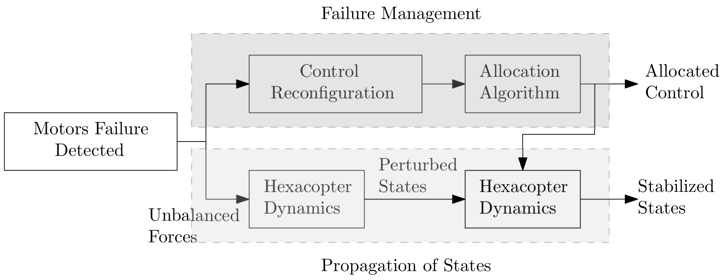
In this paper, we focus on the allocation of controls when some motors fail during flight. Figure 1 presents a block diagram of the motor failure management process, and this paper mainly focuses on the failure management portion, presented in the block of dark gray background. Assume that motors have failed during flight and that this failure has already been detected. The uneven distribution of forces results in the offset of the states from the nominal hovering states. For hovering states, the control reconfiguration algorithm generates new control distribution regarding functional motors. However, the perturbed flight states require more control effort than do nominal flight states. The extra control effort is managed and generated by applying the allocation algorithm detailed in Figures 3 and 4. The control allocation algorithm along with reconfigured nominal control is expected to restabilize the hexacopter during hovering flight. If not, this algorithm is expected to sufficiently stabilize the flight so that pilots can perform an emergency landing.
There are three main advantages in using allocation of controls. First, only one control gain is required, even with failed motors; secondly, onboard emergency response is possible; thirdly, development process of controller is faster. Implementation of controllers requires a computing unit and other supporting components in an integrated circuit board, such as an onboard computer or a set of microchips. For a drone using an onboard computer, change of control gain or control law in response to failed motors may require an external, special device to “burn” parameters into the onboard computer, such as Pixhawk. Therefore, in general, parameters and control algorithms are not adjustable during flight in such cases. Although some computing units composed of microchips may modify their control parameters in flight, this process needs to be manipulated from the ground station. In contrast, the algorithm of control allocation along with control reconfiguration can be written in the onboard computing unit in advance. When encountering a motor failure event, the drone can respond to the emergency and stabilize itself autonomously. An alternative but similar manipulation is to prepare multiple control gains or control laws onboard, as suggested in this paper suggested with allocation matrices. This method requires longer developing period to develop, simulate, and verify controllers for various motor failure cases. Moreover, gain scheduling should also be considered for different controllers subject to change in drone configuration or variations in flight conditions. One set of control gain with the proposed allocation algorithm significantly shortens and simplifies the development process.
Specifically, the objective was to develop an approach that can be applied to safely land a hexacopter with one or more failed motors. In some cases, however, emergent and immediate landing may be difficult. Trajectory control with some failed motors is crucial under these circumstances. Assuming that failed motors are detected, our investigation focuses on control reconfiguration and control allocation. Instead of rotational speeds, force and moments are adopted as the control input in the equations of motion (EOMs). The force and moments are then distributed to the rotors. In cases in which some rotors have failed during flight, the required force and moments are allocated to the remaining functional motors if possible. This approach tolerates uncontrollable yaw but not uncontrollable pitch or roll, which is highly related to flight safety. According to our research, pitch or roll would become uncontrollable only if four or more motors fail. Therefore, this paper discusses situations involving the failure of only one, two, or three motors; such failures can be grouped into seven cases. The paper also proposes a general allocation algorithm for efficiently allocating thrust and moment loads to the remaining functional motors even when non-full-rank control allocation matrix is applied. Thus, the designated control law and control gain need not be changed due to motor failure. This assumption is relatively practical because change of control law or control gain takes relatively larger effort as discussed previously. Our algorithm considers the control of full states, including trajectory and attitude, and is verified through numerical simulations.
The rest of this paper is organized as follows: Section 2 describes the dynamics and EOMs. The applied control law and the general control allocation algorithm are presented in Section 3. In this paper, our algorithm applies a linearization approach for equation analysis and simulations are conducted in a nonlinear regime to demonstrate the validity of the algorithm. Section 4 discuses cases of failed motors and failure management. Several simulations are presented in Section 5 to verify the proposed algorithm. The final section concludes our work and summarizes the contributions.
2. Dynamic Model of the Hexacopter
2.1. Coordinate System and Rotor Numbering
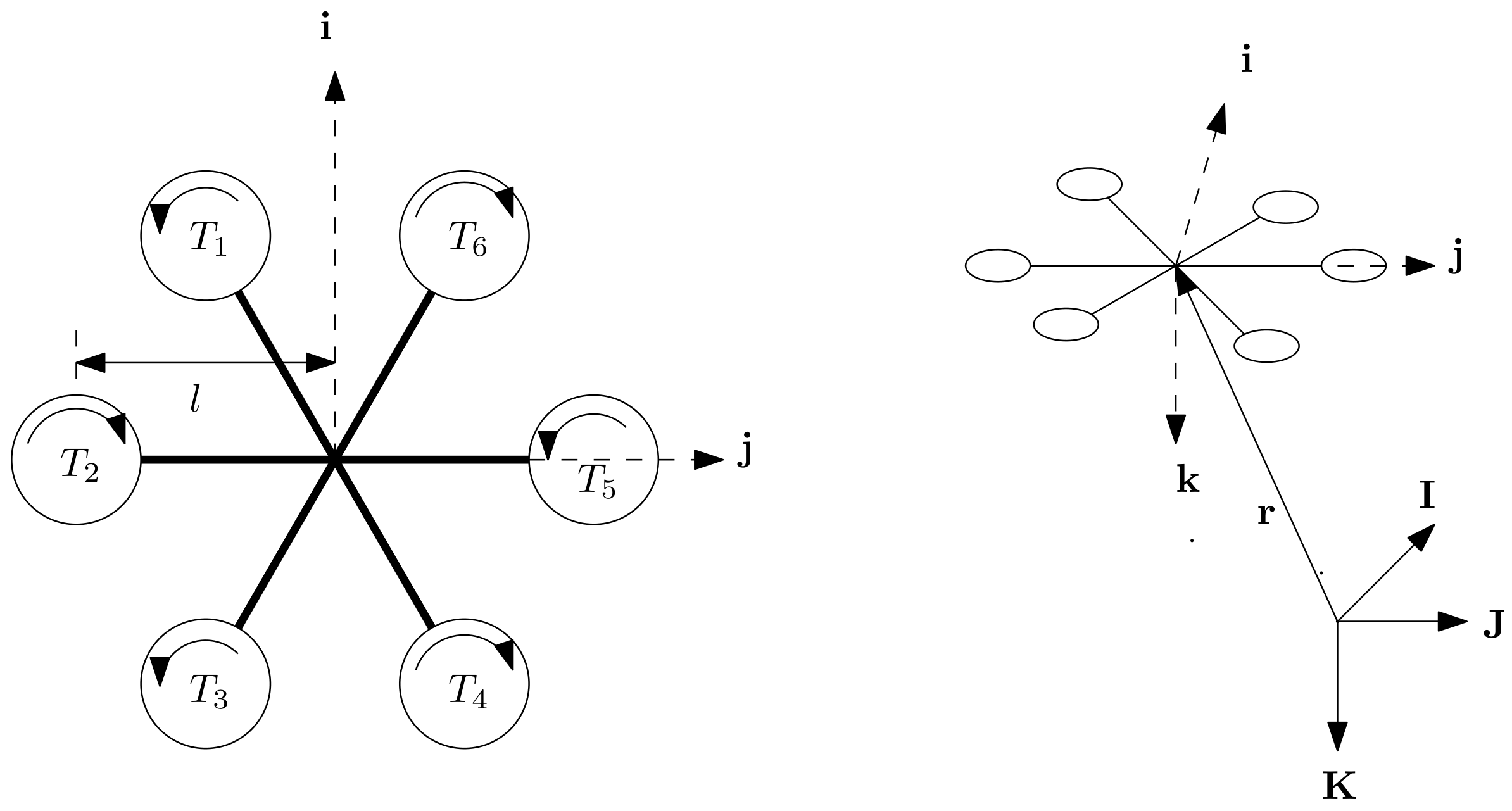
A hexacopter is composed of six rotors. To keep the momentum of the whole vehicle neutral, the six rotors are arranged in three pairs, with the two rotors in each pair rotating in opposite directions (Figure 2, left panel). The six rotors are separated form one another at an angle of 60°.
A Cartesian coordinate system, comprising the axes , with origin at the center of mass (CM) of the hexacopter is defined for further investigation. Because this coordinate system shifts along with the hexacopter, it is in the drone body-fixed frame (BF). The -axis is defined so that the left rotor rotates counterclockwise (CCW) and the right rotates clockwise (CW) from the top view. Because the vehicle is rotationally symmetric, the direction can be arbitrarily assigned as long as the aforementioned constraint is satisfied. The -axis points rightward and is perpendicular to the i-axis. Finally, completes the triad.
A local-vertical-local-horizontal (LVLH) frame, comprising the axes , is also defined. The -axis points northward, -axis points eastward, and -axis points toward the center of the earth. Because the endurance of a hexacopter is much shorter than a day, the earth can be assumed to be static during a mission, and the LVLH frame can be regarded as inertial. A diagram depicting the concept is presented in the right panel of Figure 2.
A set of Euler angles is employed to describe the rotation of the hexacopter, representing the rolling, pitching, and yawing angles, respectively. Throughout this paper, we adopt a yaw-pitch-roll sequence, also called 321-sequence, for rotations from the LVLH (inertial) frame to the BF. A rotation matrix associated with the set of Euler angles is defined to transform coordinates of a vector with respect to the LVLH frame to those with respect to the BF. Detailed formulation of can be found in [22]. A rotation matrix is orthonormal, satisfying . Additionally, a matrix is employed to transform an angular velocity to the time change rate of Euler angles , described by Equations (2) and (3) [22].
For further investigation, all rotors are assigned a number. All rotors in the CCW direction from the -axis are designated as to , as depicted in Figure 2.
2.2. Hexacopter Dynamics
Let denote the position of the hexacopter with respect to the LVLH frame and be the velocity of the CM. Accordingly, the kinematic equations can be expressed as follows:
where , and
In Equation (3), and . Notably, and are expressed in different coordinate systems. A rotation matrix should be applied to Equation (1) in actual computation processes. Moreover, is not a rotation matrix, and singularities exist when . A hexacopter usually flies with a small pitch angle and is not influenced by singularities. An alternative solution to avoid singularity is the employment of quaternions.
The kinetic equations can be derived from Newton’s laws of motion. Let be the external forces exerted on the hexacopter and be the external moments with respect to the CM. Newton’s second law of motion describes the following:
where is the inertia tensor with respect to the CM in the BF. Because a hexacopter is usually symmetric to the and planes, the inertia tensor can be expressed as .
Formulation of Forces and Moments
A previous study detailed the formulations of forces and moments [23], and the results of these formulations are cited herein directly. However, the formulations must be slightly modified because some definitions in this paper are unique.
The total force exerted on the hexacopter can be divided into four components: the thrust , rotor drag , air resistance , and weight . Therefore,
According to [23], the aforementioned forces can be formulated as follows:
where b is the thrust factor, is the rotational rate of the ith rotor, is a constant, is the atmospheric density, is the drag coefficient, and S is the reference area; moreover, .
The moments and torques comprise four sets: torques due to rotational rate difference between rotors , torques due to gyroscopic effects , and yaw counter torque [24,25]. Hence,
where . , , and denote the roll, pitch, and yaw moments, respectively and can be further derived as follows:
where d is the drag factor, and l is the distance of rotors from the CM, as illustrated in Figure 2. and are formulated as follows:
where is the rotational inertia of the propeller, and is the overall propeller speed.
2.3. Hexacopter Nonlinear EOMs
The EOMs of a hexacopter are given by Equations (1), (2), (4) and (5), and expansion of these equations are provided in Equations (A1)–(A12) in Appendix A. Define a state vector as follows: . Equations (A1)–(A12) can be summarized as follows:
where are the equations and is the control vector.
In this paper, two aspects of control inputs can be considered: the rotation rates of rotors and the force-moment set. In the first case, , where denotes non-negative real numbers; accordingly, the rotation rates of rotors are used as control inputs. In the second case, ; accordingly, the lift force as well as three moments are used as control inputs. The two control vectors are convertible and are employed in different scenarios.
Notably, in the EOMs. This may increase difficulties in further analysis because the control is constrained. We perform a change of variable by defining , where for . This definition leads to
Then,
Moreover, is replaced by for further analysis.
2.4. Linearization of EOMs
2.4.1. Equilibrium Point
As mentioned, the aim of this paper is to develop an algorithm for the analysis and management of hexacopter motor failures. When a hexacopter incurs a rotor failure during flight, an emergent hovering is designed to be imposed, and the developed algorithm can be applied to manage the failure. After control is regained for the hexacopter, the hexacopter may continue its designated trajectory or perform an emergency landing. Therefore, the proposed algorithm can help regain hexacopter controllability during hovering.
The equilibrium state during hovering is expressed as follows [26]: . Therefore, the following can be derived: , , and . Notably, the system does not execute maneuvers during hover, implying that and .
2.4.2. Nominal Control for Equilibrium
Alternatively, , where the bar over a variable denotes evaluation in nominal states, and the subscript “0” denotes no failed motor. is a transformation matrix that transforms to .
To simulate the failure of motors, an effectiveness matrix is employed. is defined as , where represents the status of the motor i. In this paper, we only allow motors to be on or off. As a result, for a normal motor and for a failed motor. Then Equation (24) can be generalized as . Or, by letting .
Let
where represents the first row and represents the remaining entries of . Consequently, subject to the following constraints:
where denote the null space of a matrix. Notably, if .
Conclusively, the solution space is
where Sp is the span of the vectors, , , , and are coefficients.
In some cases, however, full control of the system in the nominal level is impossible. An alternative strategy is to release the yaw constraint. Since emergent safe landing is the first priority of the goal, sacrificing yawing motion is safer than sacrificing pitching or rolling motion of a multirotor craft. With this assumption, the third row of is removed. Denote the new matrix as , and its null space is given by
where , , , , and are coefficients.
2.4.3. Linearized EOMs
The linearized system is expressed as follows: , where the state matrix is , and the control matrix is or . and can be derived through partial differentiation with respect to and evaluated at the equilibrium point, and calculations are provided in Appendix A.
3. Control Allocation
3.1. Control Architecture
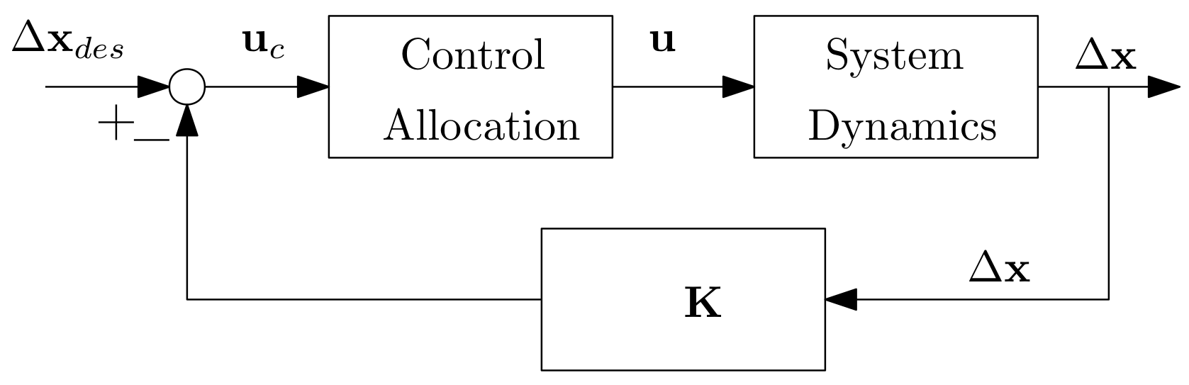
Feedback control laws are usually designed to stabilize a hexacopter and can generally be presented as follows: , where denotes the feedback gain, denotes the real-time state vector, and denotes the desired state vector. A different control law may result in a different gain .
The control allocation architecture is shown in Figure 3, where . Let denote the control command computed from the control law. As mentioned, is given by lift force and three moments. In practice, the control signal should be allocated to and realized by the rotational speed of each rotor. The rotation of rotors in response to the control command then generates corresponding lift and moments, denoted as u, to stabilize the hexacopter.
If all motors function well, the allocated rotational speeds should be identical to the actual rotational speed, leading to . If some motors fail, only the remaining operational motors can generate controls. Consequently, in such cases. The proposed algorithm forces for failed motors by reallocating control to the remaining motors if possible—the limitation of the algorithm.
3.2. Transformation of Controllers
The transformation of and in the linear regime can be obtained by linearizing Equations (19)–(22) for the nominal rotational rates. Let and . The transformation can be written in matrix form as follows:
where
where . Here we name W as a “linear transformation matrix”, which transforms to .
In the implementation, is applied to prevent the adjustment of control gains due to motor failures. To compensate for the loss of the failed motors, the control commends are allocated to the remaining functional motors. Hence, we specify as because is the control vector obtained from the control law. is renamed as for simplicity. Moreover, we drop the -sign in the following derivations for simplicity, leading to . Notably the following derivations are only linear approximations. Nominal controls should be considered and added if the original full nonlinear system is to be simulated. Moreover,
3.3. Control Allocation in General Situations
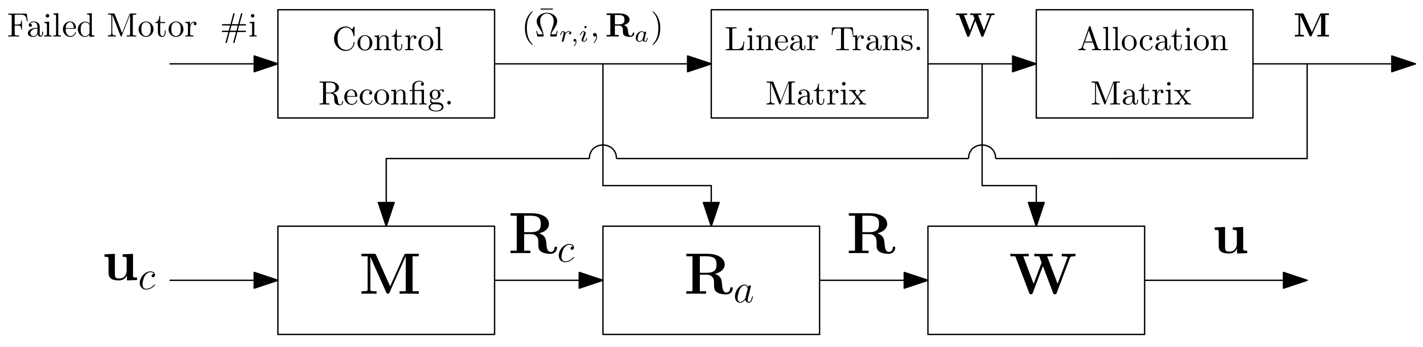
Figure 4 presents the flowchart of the control allocation algorithm. The subscript “c” denotes the command derived from the control law, and a term without a subscript denotes the actual input in the implementation. Given a control command , the command for the rotational speeds can be derived by multiplying the allocation matrix , given by . On the other hand, if the ith motor is failed. Multiplied by , simulate the actual rotation of rotors. For example, given the first and third motors fail, we obtain the effectiveness matrix and the corresponding .
According to Equation (30),
In normal flight, , and . When some motors fail, the design of the allocation matrix becomes critical. The following questions are assessed in this paper:
- Does exist so that when some motors fail?
- If yes, what is the best method to design ? if no, what is the best method to regain the control of the hexacopter?
3.4. Controllability of the System
When some motors fail during flight, the designated control command cannot be fully realized, causing loss of force and unbalanced moments. An ideal allocation algorithm will redistribute the rotational speeds of the remaining operational motors so that the lost thrust is compensated for. Obviously, not every failure situation can be compensated for. For example, in the special case that all six motors fail, the thrust will never be compensated for. Therefore, the effectiveness of the allocation algorithm depends on whether the system is controllable subject to a constrained control.
The controllability of the system in the specific allocation problem can be formulated as follows: consider a linear control system
In our problem, the details of the state-space equations are presented in Appendix A. The controllable states and the corresponding control must be determined, and the domain of the actual control is given by
Recall that , leading to , where denotes the range space of . Because and , .
4. Failure Management
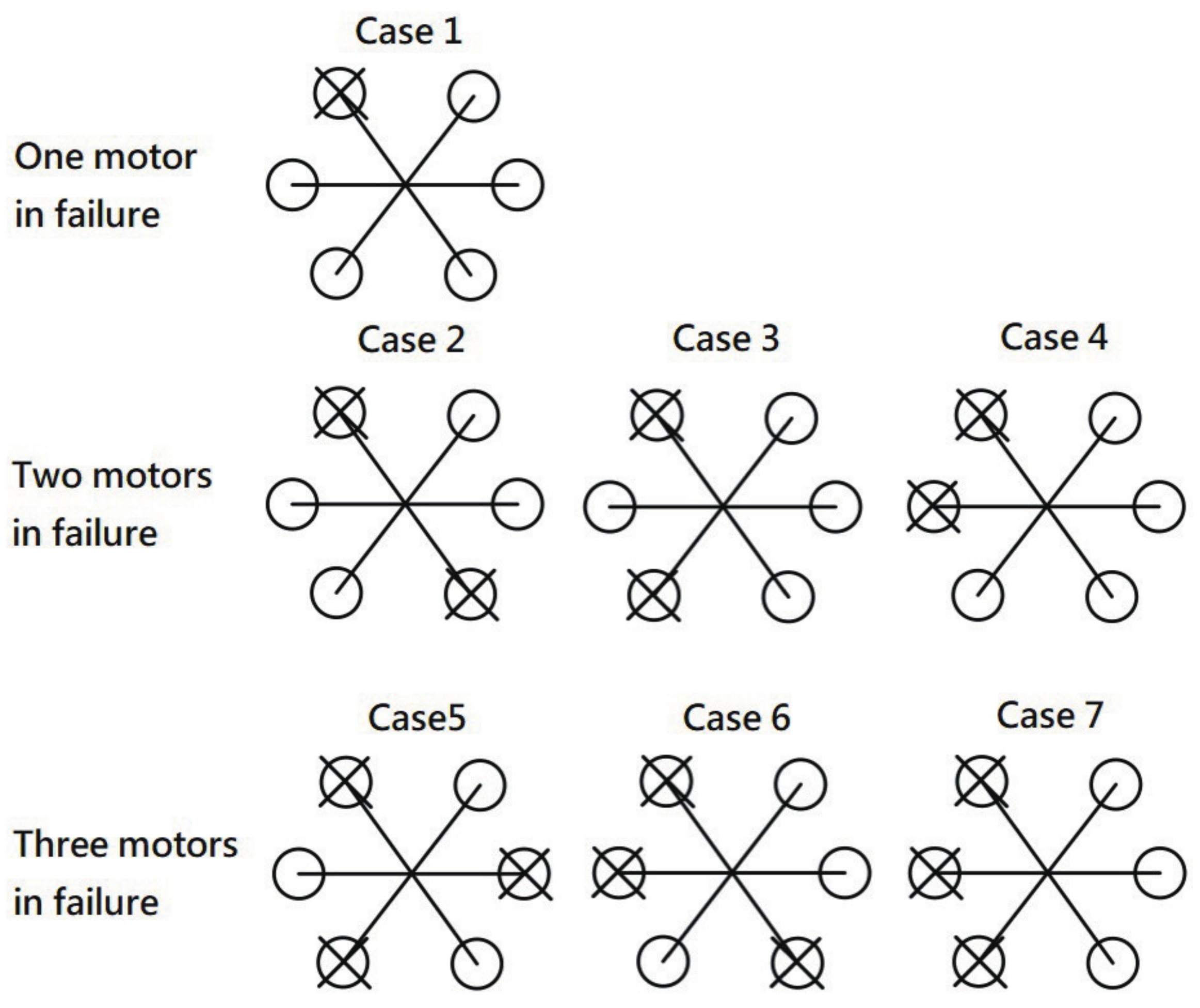
In this paper, we consider seven cases of motor failure: one case involving only a single failed motor, three cases involving two failed motors, and three cases involving three failed motors. The arrangement of the subsequent failed motors is based on motor 1 because the arrangement of the six motors on the hexacoptor is geometrically symmetrical. The failure cases are illustrated in Figure 5. The crosses on the motors signify that the motors have failed.
4.1. Design of Allocation Matrix
Failure management is discussed in this section. Once failed motors are detected, the allocation matrix is adjusted to reallocate required rotor rotational speeds so that the designated control inputs can be realized. Because the function of is to maintain , the following identity holds:
Let denote the failed motors. For example, If Motors #1 and #4 fail, then and . If all motors function normally, that situation is denoted by . On the basis of this definition, Equation (36) can be further simplified as follows:
Taking the right pseudo-inverse of yields
In the case that is singular, implying that full control of the hexacopter is impossible, the yaw control must be sacrificed. Let
where and . If rank=3, is invertible. Then, is constructed as follows:
Accordingly,
With such , we can determine that , , and , but . Although the yaw control is not as designed and may fail to control the yaw motion, this situation is acceptable: first, the yaw motion is independent of other states in the linear sense, and failure in yaw control does not affect the propagation in other states; second, uncontrolled yaw motion does not influence the flight safety considerably whereas uncontrolled pitch or roll motion may cause a crash.
If rank, flight safety cannot be achieved for the hexacopter. These cases are out of the scope of this paper and are not discussed.
4.2. Case 0: Control Allocation in Normal Flight
4.2.1. Allocation Matrix Design
Assume that all motors are normal. The nominal rotor rotation rates are , and . The allocation matrix is attainable via Equation (38) and provided in Equation (A22) in Appendix B.
4.2.2. Controllability
A system without failed motors must be fully controllable. This fact can also be proved as follows:
The controllability matrix formed by the pair is full rank, indicating that all states are controllable.
4.3. Case 1: One Failed Motor
4.3.1. Reconfiguration of Rotor Rotation
Without loss of generality, we can assume that Motor #1 failed during flight. In this case, nominal control is attainable by solving Equation (27) with a vector in Equation (28) subject to the constraint: . One solution is , where . As a result, nominal control can be derived as follows: , resulting in .
4.3.2. Allocation Matrix Design
In this case, , and is attainable by . The 1st and 4th columns are zeros, and this indicates that rank. The allocation matrix is attainable via Equation (40) and provided in Equation (A23) in Appendix B.
4.3.3. Controllability and Stabilizability
The control matrix is expressed as . The structure of is identical to Equation (A17), and that of identical to Equation (A20). However, is modified as follows:
We can derive the controllability matrix and assess the rank. Rank. Hence, this is an uncontrollable system. This result is consistent with those proposed in [12]. An alternative approach can be achieved by defining the controllability matrix as follows:
where is an eigenvalue of . Those uncontrollable eigenvalues reduce the rank of . has ten unstable eigenvalues at 0 and two stable eigenvalues at . By scanning through all eigenvalues of , we conclude that the system is unstabilizible because the uncontrollable eigenvalues are the 0 values.
According to control theory, controllable states can be found in the column space of , denoted as . Executing manipulations yields
where is a standard basis in the vector space, and
The subscript denotes a failed motors. This result explains that only specific initial conditions in the yaw motion can be stabilized when our algorithm is applied in a case in which opposite motors have failed.
4.4. Case 2: Two Opposite Motors Fail
In this case, two opposite motors are assumed to have failed, as shown in Figure 5. Without loss of generality, we use Motor #1 and #4 as an example. Other opposite pairs of failed motors lead to similar results.
In this case, and for . . The parameters in this scenario are identical to those in Case 1. Therefore, the analysis procedures and results are also identical to those in Case 1.
4.5. Case 3: One Working Motor in Between
In this case, we assume one working motor in between two failed motors, as shown in Figure 5. Without loss of generality, this paper uses failed Motors #1 and #3 as an example.
4.5.1. Reconfiguration of Rotor Rotation
4.5.2. Allocation Matrix Design
In this case, , and is attainable by . Only the 2nd and 5th columns are nonzeros, and this indicates that rank. Accordingly, pitch and roll are uncontrollable. Hence, this scenario is out of the scope of this paper.
4.5.3. Alternative Reconfiguration
An alternative way to reshape nominal control is to release the stability of yawing motion. In this circumstance, nominal control is attainable by solving solving Equation (27) with a vector in Equation (29) subject to the constraint: . One solution is , where . Consequently, according to Equation (27), nominal control can be derived as follows: .
4.5.4. Controllability and Stabilizability
The control matrix is calculated as . The structure of is identical to Equation (A17), and those of and are identical to Equations (A20) and (A21), respectively. Because Equations (A20) and (A21) are derived under the assumption of normal flight, the system is controllable.
Notably, the system is controllable because we restricted our attention to stabilize yaw motion. The system should be controllable if and only if yaw stability is not considered. In contrast to Case 1 and Case 2, in which the yaw motion is uncontrollable at the linearized level, yaw stability is not considered at the nominal level in this case. Therefore, we can expect the divergence of the yaw motion to be greater and faster than those in Case 1 and Case 2. The allocation matrix is provided in Equation (A24).
4.6. Case 4: Adjacent Motors in Failure
In this case, two adjacent motors are assumed to have failed, as shown in Figure 5. Without loss of generality, we consider Motors #1 and #2 as examples.
4.6.1. Reconfiguration of Rotor Rotation
4.6.2. Allocation Matrix Design
In Case 4, , and is attainable by . Only the 3rd and 6th columns are nonzeros, and this indicates that rank. Accordingly, pitch and roll are uncontrollable. Hence, this scenario is out of the scope of this paper.
The alternative approach of releasing yaw control is also investigated for this case. After a similar manipulation procedure to that in the preceding cases, we can obtain that one solution is , where . Consequently, according to Equation (27), nominal control can be derived as follows: . Since the result is identical to that in the full approach, this case is uncontrollable.
4.7. Three Motors in Failure
In this section, the three motors are assumed to have failed simultaneously. Potential cases are demonstrated in Figure 5, and they are numbered as Case 5, Case 6, and Case 7. Without loss of generality, motors #1, #3, and #5 are used as an example of failure for Case 5; motors #1, #2, and #4 are used as an example of failure for Case 6; and motors #1, #2, and #3 are used as an example.
4.7.1. Case 5: (#1, #3, #5) Motors in Failure
In this case, the only solution to Equation (27) with a vector in Equation (28) subject to the constraint is , leading to . This implies that nominal rotational rates to stabilize the hexacopter do not exist. We can thus conclude that full controllability of this system is impossible.
An alternative approach is to release the constraint in yawing. With this assumption, we conclude that , where . According to Equation (27), nominal control can be found as follows: , resulting in .
Therefore, , and is attainable by . The 1st, 3rd, and 5th columns are zeros, and this indicates that rank. The allocation matrix is attainable via Equation (40) and provided in Equation (A25) in Appendix B.
The control matrix is calculated as . The structure of is identical to Equation (A17), and that of identical to Equation (A20). However, is modified as follows:
Through a similar analysis process, we realize that this an uncontrollable and unstabilizable system.
According to control theory, controllable states can be found in the column space of the controllability matrix , denoted as . Executing some manipulations yields
where
The subscript denotes the failed motors.
4.7.2. Case 6: (#1, #2, #4) Motors in Failure
In this case, nominal control is attainable by solving solving Equation (27) with a vector in Equation (28) subject to the constraint: . The only solution is , where . This solution space is identical to the space in Case 4. Hence, the pitch and roll are uncontrollable.
Consider the alternative approach, which entails releasing the constraint on yaw at the nominal level. We obtain , where . This result is identical to Case 4, and we argue that this case is uncontrollable.
4.7.3. Case 7: (#1, #2, #3) Motors in Failure
In this case, the only solution to Equation (27) with a vector in Equation (28) subject to the constraint is , leading to . This implies that nominal rotational rates to stabilize the hexacopter do not exist. We can thus conclude that full controllability of this system is impossible.
Consider the alternative approach, which entails releasing the constraint on yaw at the nominal level. One possible solution is . Consequently, according to Equation (27), nominal control can be derived as follows: . Because all entries of the vector must be greater than zero, this approach is infeasible. Hence, we argue that this case is fully uncontrollable.
4.8. Summarization of Cases Study
After studying potential failure cases, we conclude that
- the pilot is able to regain controllability of states other than yawing motion when two opposite motors have failed;
- for the case with only one failed motor (Case 1 and Case 2), the best strategy is to turn off the opposite motor and perform the same maneuver as in the previous scenario;
- for the case with two failed motors with one working motor in between (Case 3), the pilot is able to regain controllability of states other than yawing motion. In this scenario, however, the hexacopter tends to spin and wobble severely.
- for the case with three failed motors with one working motor in between (Case 5), the pilot is able to regain controllability of states other than yawing motion. Similar to the previous scenario, the hexacopter tends to spin and wobble severely.
- for other cases, it is very markedly difficult for the pilot to regain controllability and safely land the hexacopter.
5. Numerical Simulations
5.1. Controller and Simulation Parameters
We present the simulation of an example flight mission to verify the proposed algorithm. Table 1 lists the simulation parameters of the hexacopter.
An LQR controller is designed to stabilize the linearized dynamics of the hexacopter with the three weighting matrices being set as follows:
The feedback gain in Section 3.1 is given by , where satisfies the continuous algebraic Riccati equation [27].
The initial offset in the simulations is given by , where m is the position offset, rad is the attitude offset, m/s is the velocity offset, and rad/s is the angular offset. Because we simulate a situation in which the control is subject to reconfiguration due to the sudden loss of motors, we can set the initial control offset as . For a performance comparison, these initial conditions are employed throughout the cases, except for some specific cases.
5.2. Verification of Case 0
This case represents a control scenario with no motor failure. According to the results in Section 4.2, the linearized system is fully controllable. Figure 6 illustrates that all states can converge to 0 values, which represent the nominal states. The control input is shown in Figure 7. and are identical, as predicted. The rotational speeds of the six motors are presented in Figure 8. These rotational speeds are the actual rotational speeds, computed using , where and . The speeds are identical to the nominal speeds eventually.
5.3. Verification of Case 1 and Case 2
5.3.1. Arbitrary Initial Condition
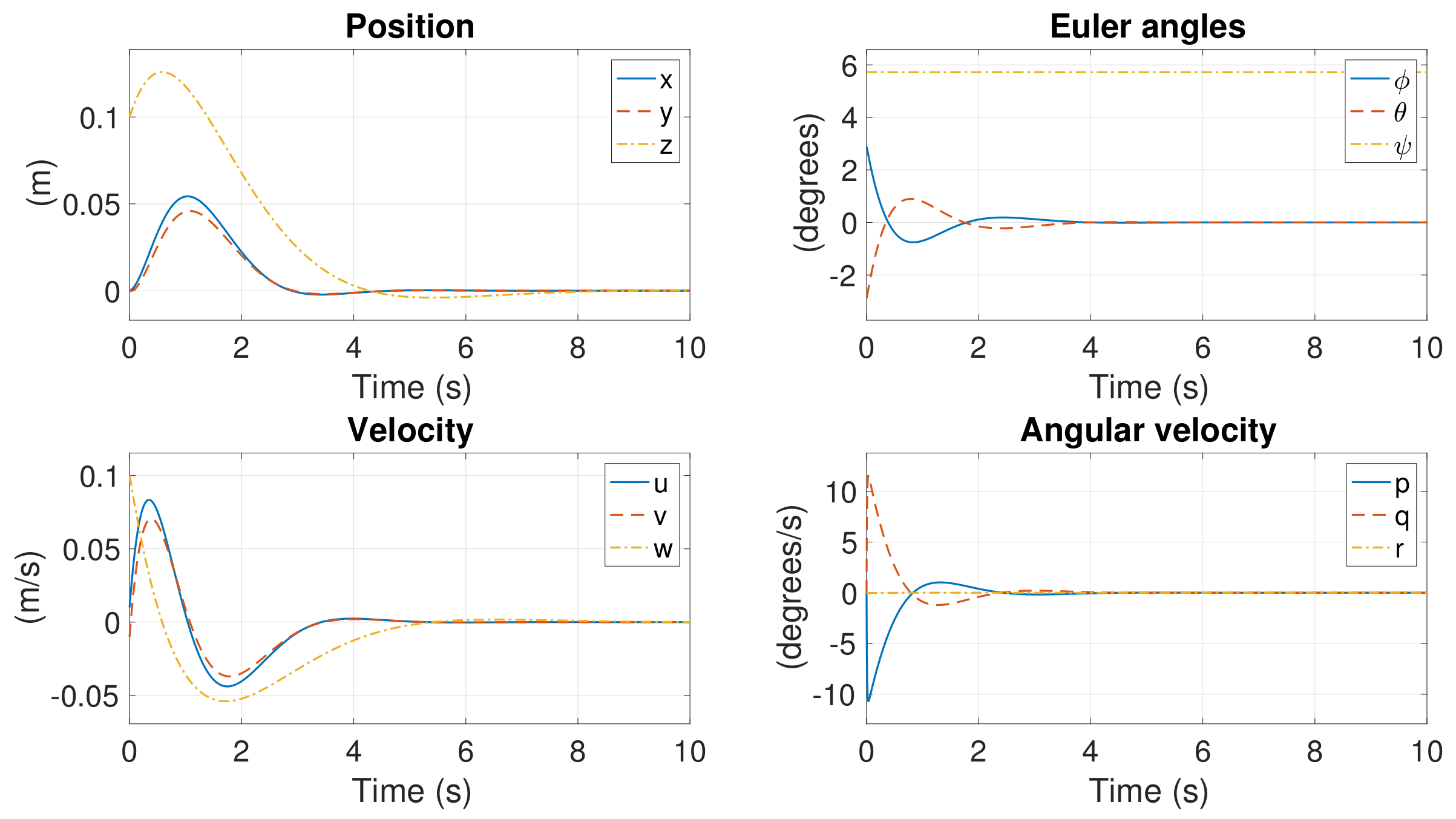
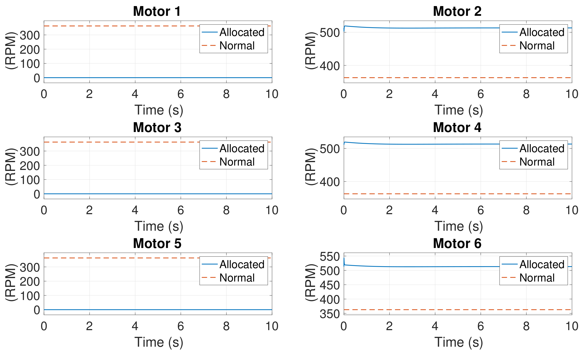
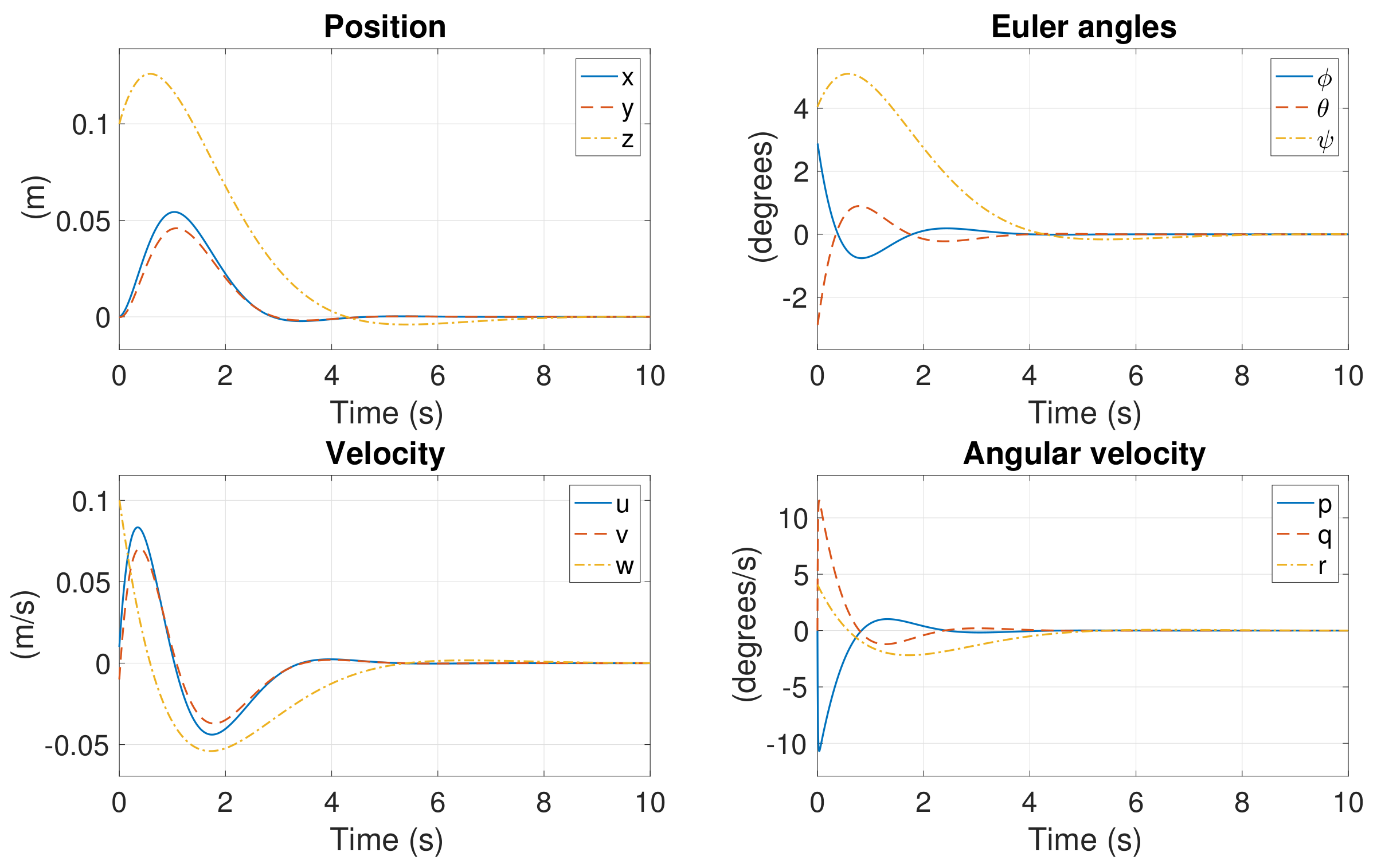
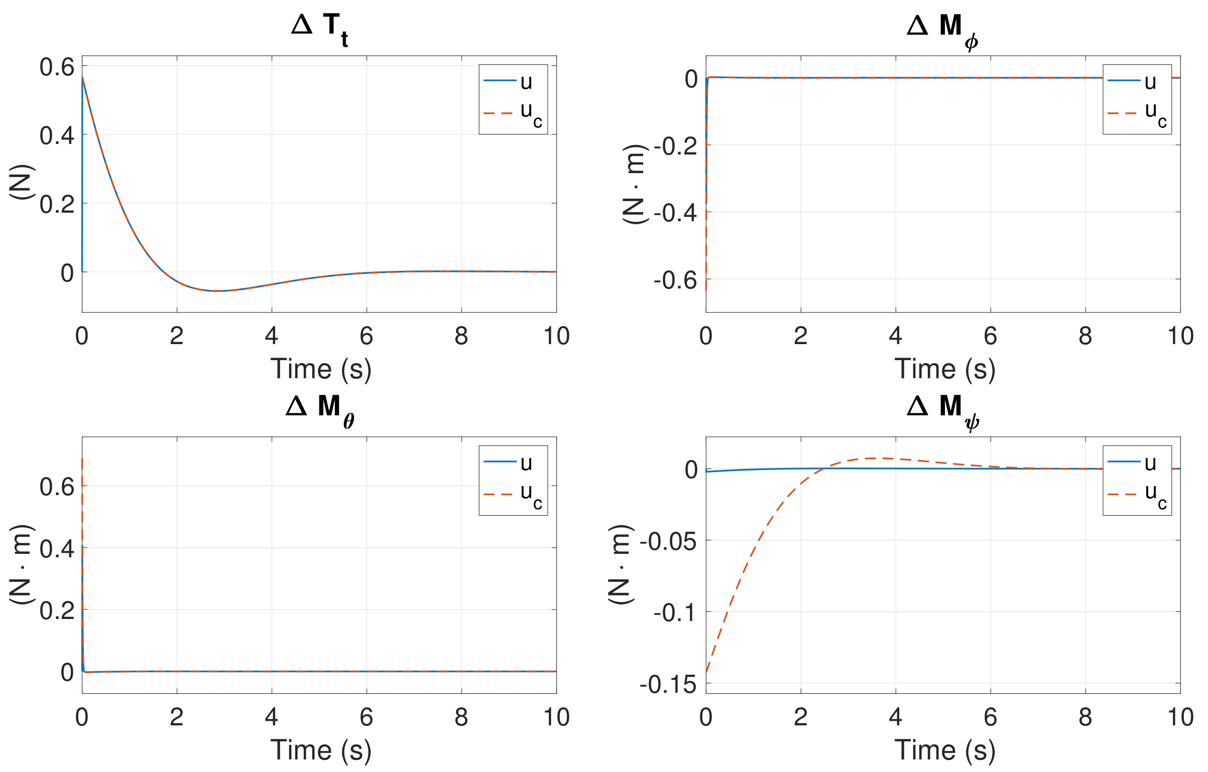
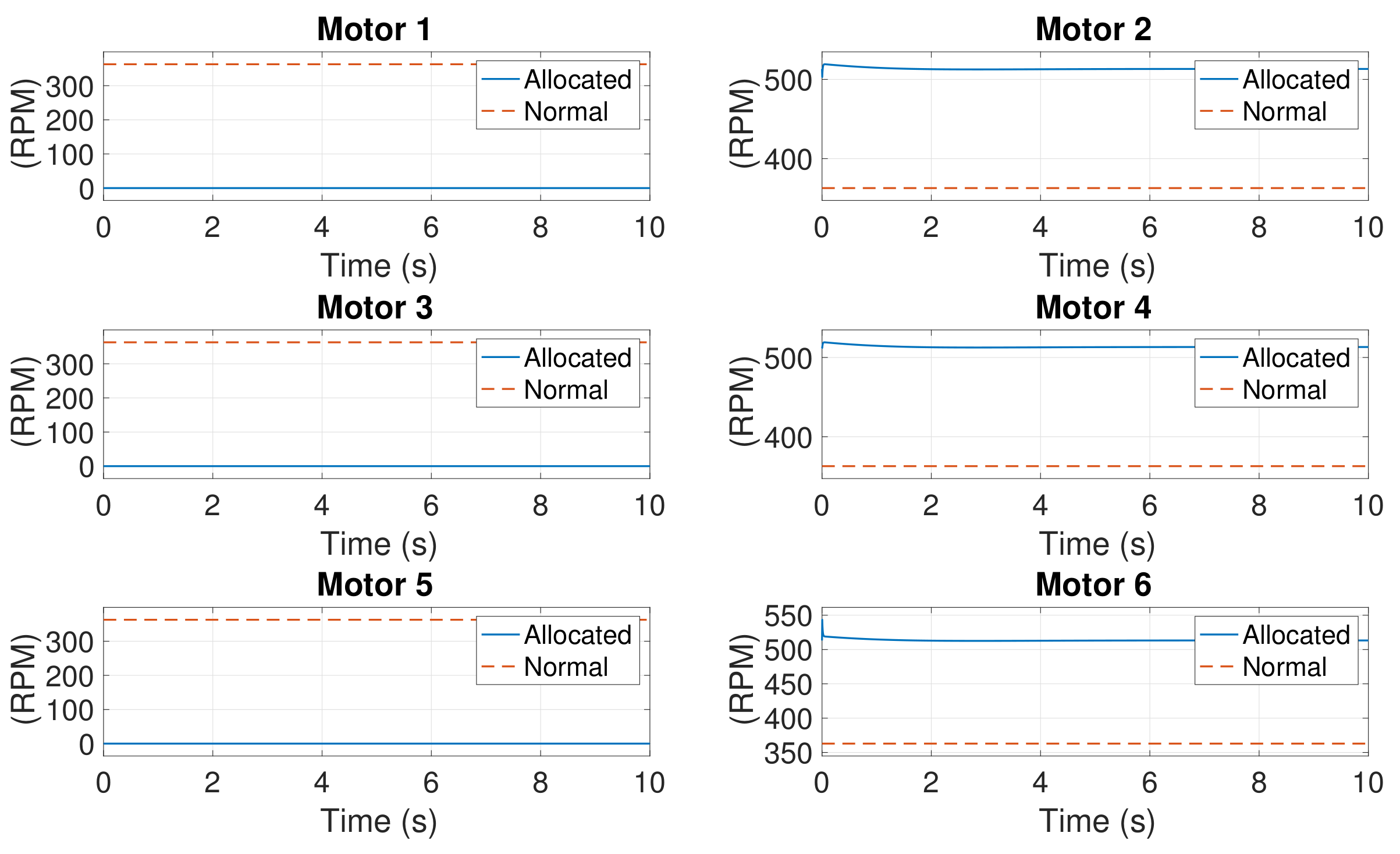
The failure of Motor #1 is simulated in this section. According to the reconfiguration result in Section 4.3, Motor #4 should be turned off to maintain the hexacopter’s balance. However, turning Motor #4 off also prevents the stabilization of the linearized system at the linear level. This scenario is identical to Case 2, where Motors #1 and #4 lost power simultaneously due to failure. The aforementioned arbitrary initial condition set is employed in this simulation. Figure 9, Figure 10 and Figure 11 present the simulation results.
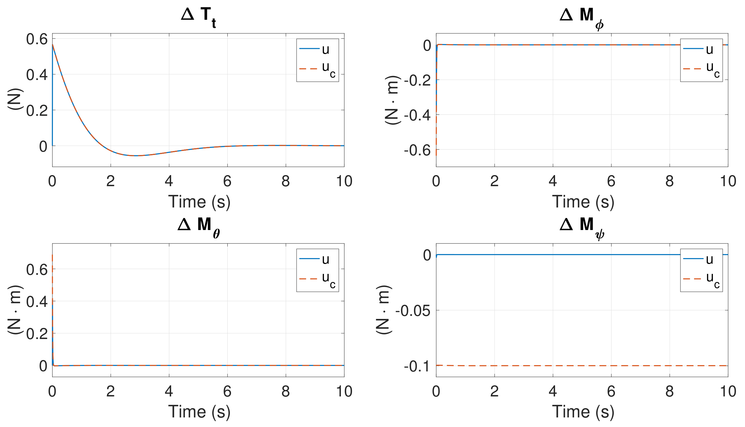
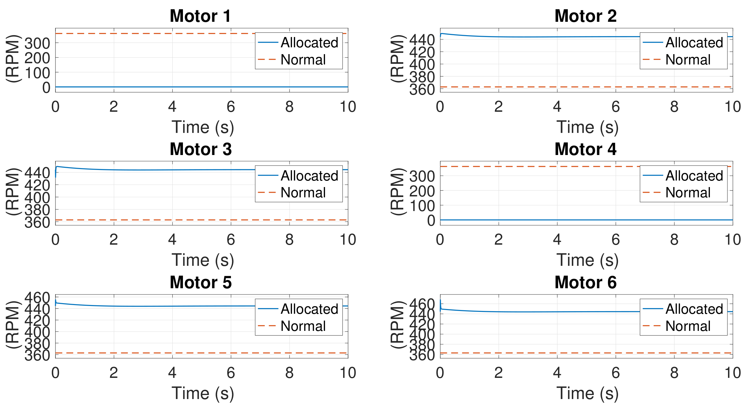
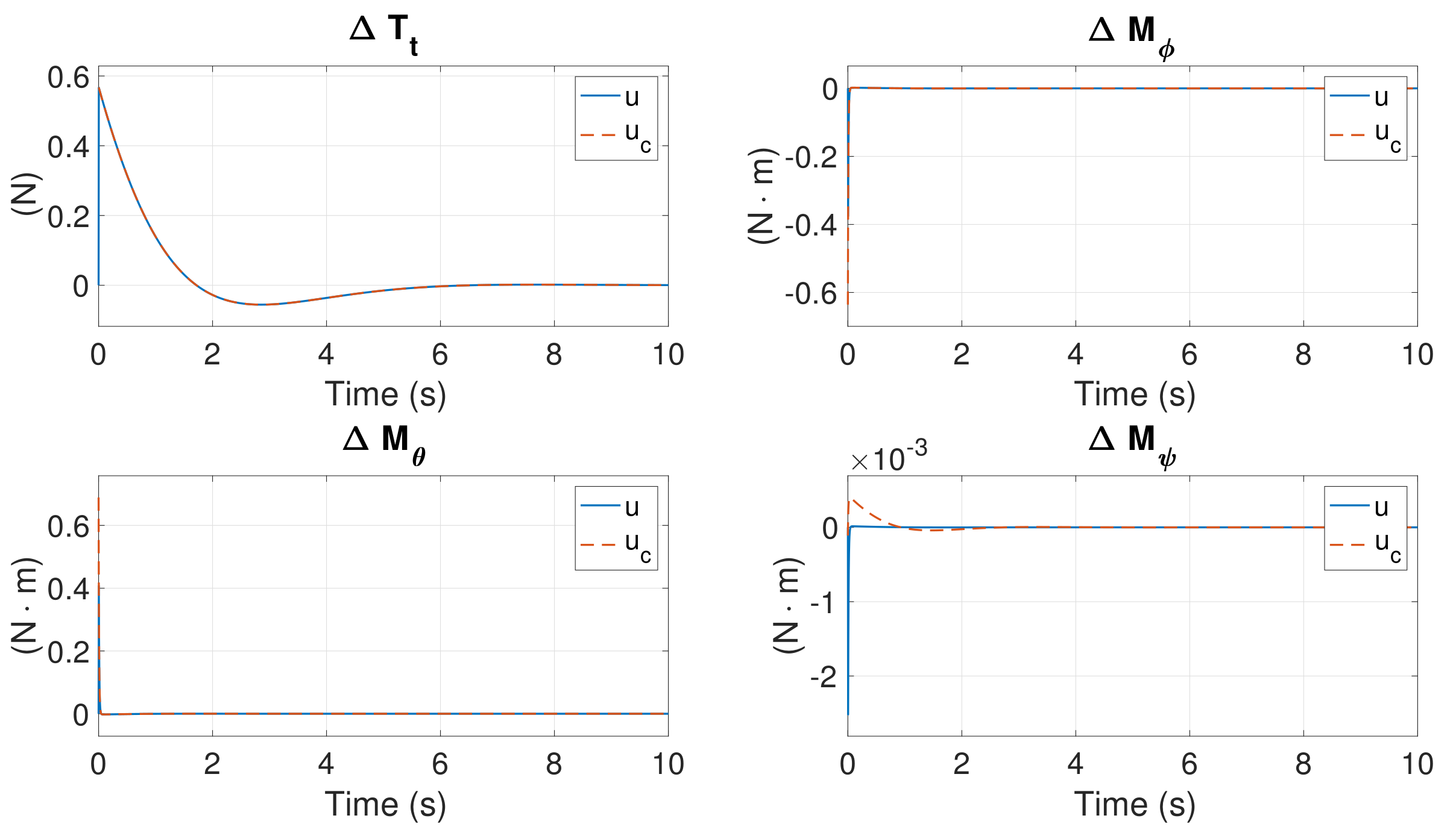
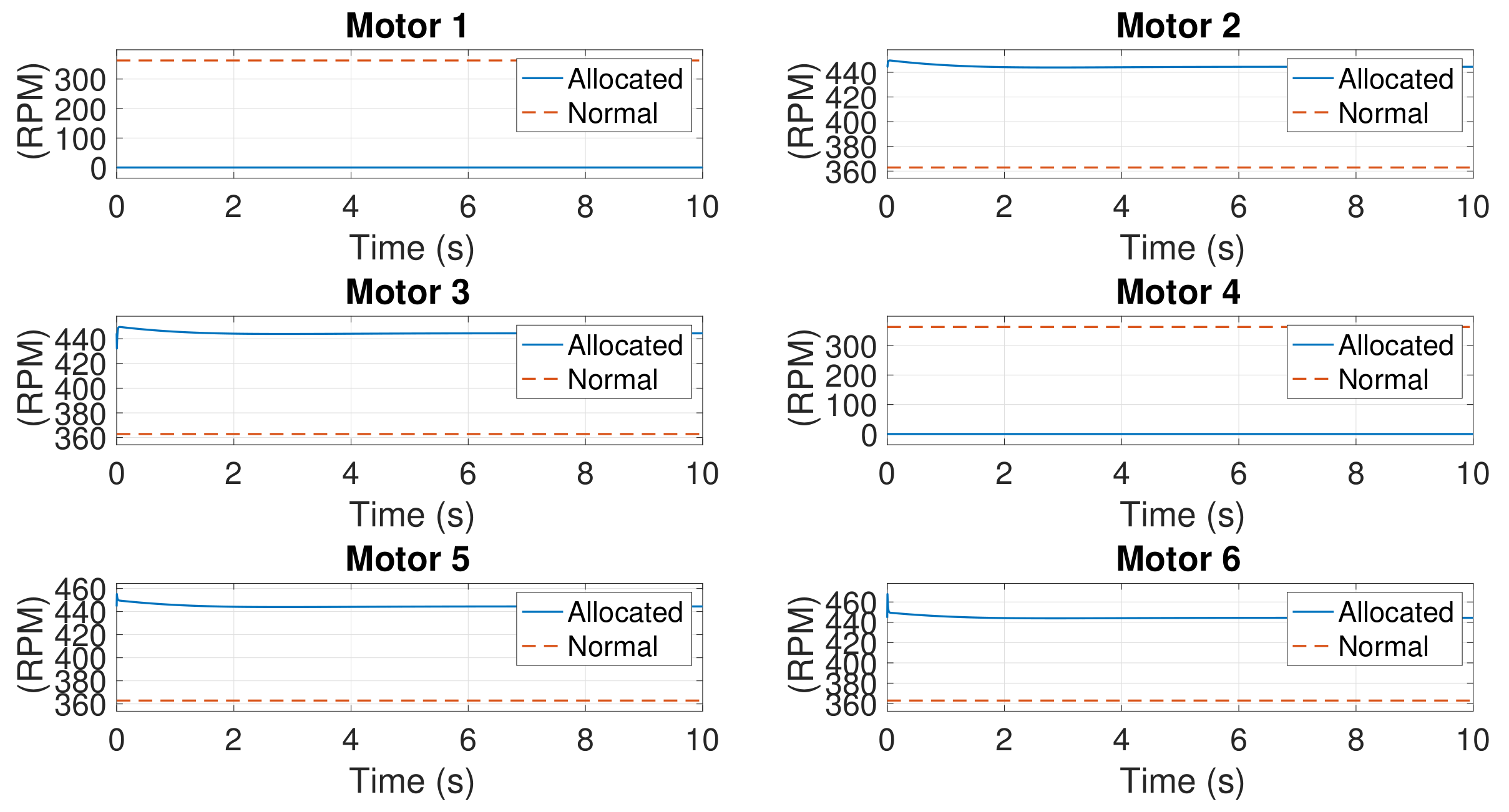
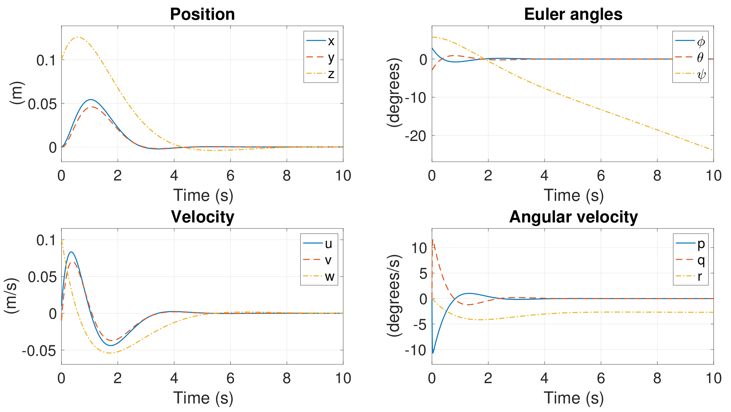
All states in Figure 9 converge to zero except . Notably, remains constant with the convergence of the yaw rate r. The control inputs are shown in Figure 10. , and are generated to control the system, whereas remains at zero due to the failure and deactivation of the motors. The rotational speeds of the six motors are presented in Figure 11. The speeds of Motors #1 and #4 are zero, and the speeds of the other motors are increased to reshape the thrust and torques.
5.3.2. Controllable Initial Condition
According to control theory, initial conditions from any controllable set in a partly controllable system should be controllable. This section presents the verification of our algorithm because it is unlikely for a hexacopter to fall into this initial condition subject to motor failure in a real flight. The controllable initial condition set is provided in Section 4.3.3.
In this simulation, are identical to the aforementioned initial conditions. However, is obtained from the corresponding element of . Similarly, is obtained from the corresponded element of . The state responses are displayed in Figure 12. All states converge to zero, including . Figure 13 shows the control response. , and are derived to control the system, whereas remains at zero due to the failure and deactivation of the motors. These results demonstrate that is controllable even if is not available or derived. The rotational speeds of the six motors are presented in Figure 14.
5.4. Verification of Case 3
The simultaneous failure of Motors #1 and #3 is simulated in this section. According to the analysis in Section 4.5, the yaw motion is uncontrollable at the nonlinear level. Therefore, to maintain the safety of the hexacopter, we must give up the yaw motion and try to stabilize other states. Through this strategy, all states other than the yaw motion should be controllable.
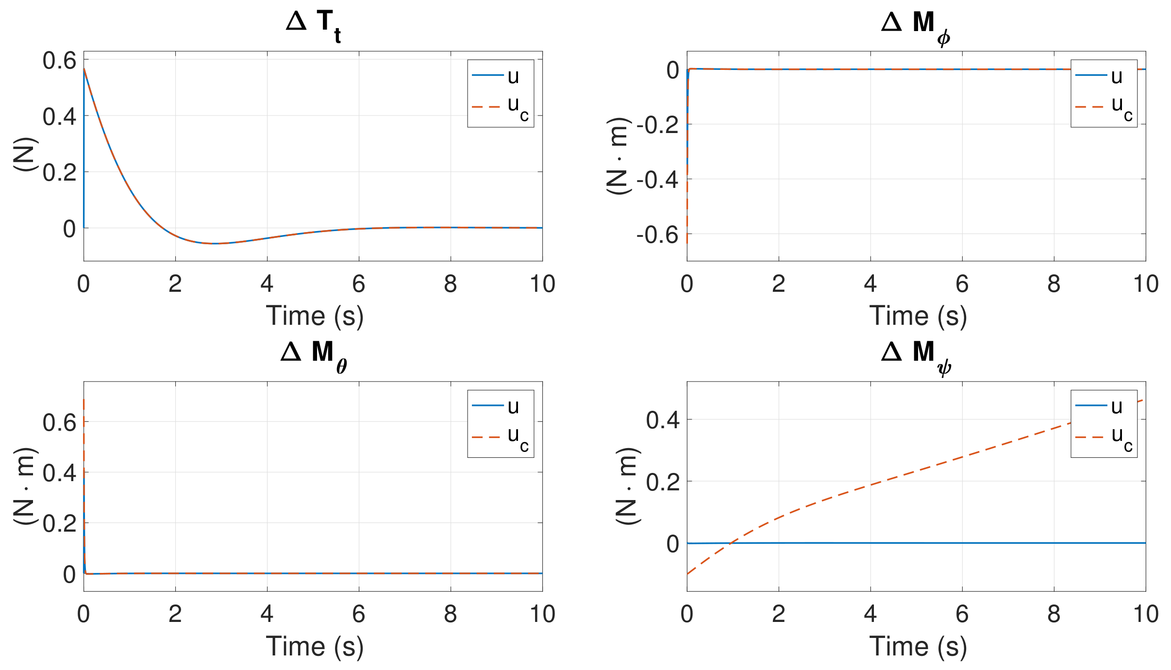
The aforementioned arbitrary initial condition set is employed in this simulation. Figure 15, Figure 16 and Figure 17 present the simulation results. Figure 15 converge to zero except and r. The control inputs are shown in Figure 16. Unlike Case 1 and Case 2 where r converges to zero and remains constant, in the present scenario, r converges to a constant and diverges.
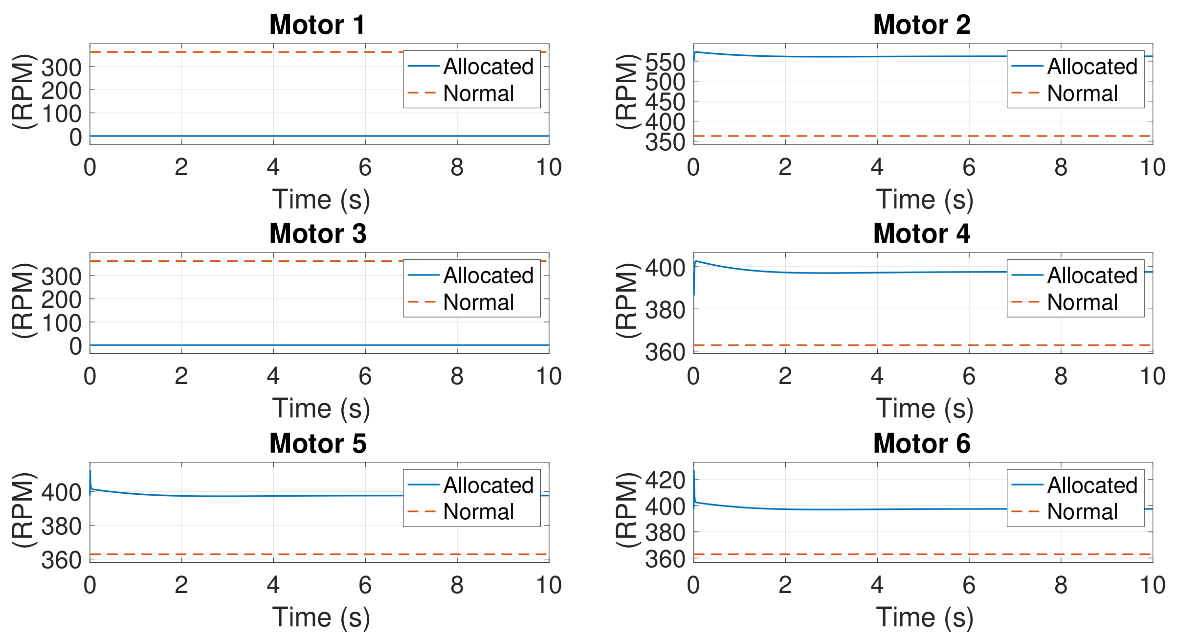
As for the control inputs, we sacrifice the yaw moment to save other states. Hence, maintains divergence, whereas , , and function normally. The rotational speeds of the six motors are presented in Figure 17. The speeds of Motors #1 and #3 are zero, and those of the others are increased to reshape the thrust and torques. Moreover, the nominal speed of Motor #2 is times more than those of Motors #4, #5, and #6.
5.5. Verification of Case 4
The simultaneous failure of Motor #1 and #2 is simulated in this section. According to the analysis in Section 4.6, this system is uncontrollable at both nonlinear and linearized levels. Figure 18 presents a simulation with the aforementioned initial conditions. All states diverge considerably fast.
5.6. Verification of Case 5
According to Section 4.7.1, Section 4.7.2 and Section 4.7.3, only Case 5 has limited controllability over the failed hexacopter. The proposed algorithm has the capability of predicting uncontrollable systems, as demonstrated in Section 5.5. Therefore, this section simulates potential responses in Case 5, where Motors #1, #3, and #5 are assumed to have failed simultaneously.
5.6.1. An Arbitrary Initial Condition
Similar to Case 3, demonstrated in Section 5.4, the yawing motion is uncontrollable at the nonlinear level. Therefore, to maintain the safety of the hexacopter, we must give up the yawing motion and try to stabilize other states. With this strategy, all states other then yawing motion should be controllable.
The aforementioned arbitrary initial condition set is employed in this simulation. Figure 19, Figure 20 and Figure 21 present the simulation results. All states in Figure 19 converge to zero except and r. The control inputs are graphed in Figure 20, similar to the responses in Case 3.
For the control inputs, we sacrifice the yaw moment to save other states. Hence, is maintained in a state of divergence, whereas , , and function normally. The rotational speeds of the six motors are presented in Figure 17. The speeds of Motors #1, #3, and #5 are zeros, and others increase their speeds to reshape the thrust and torques.
5.6.2. Controllable Initial Condition
As aforementioned, this section is merely to verify our algorithm, because it is very unlikely for a hexacopter to fall into this initial condition subject to motor failure in a real flight. The controllable initial condition set is provided in Section 4.7.1.
In this simulation, are identical to the aforementioned initial conditions. However, is obtained from the corresponding element of . Similarly, is obtained from the corresponding element of . The state responses are shown in Figure 22. All states converge to zeros, including . Figure 23 shows the control response. , and are generated to control the system, whereas maintains zero due to the failure of the motors. One can see that is controllable even thought the system has zero . The rotational speeds of six motors are presented in Figure 24.
5.7. Simulations in Nonlinear Regime
5.7.1. Formulation of Nonlinear Controller
In our previous analysis, most cases are uncontrollable for yawing motion. At the nonlinear level, attitude dynamics is coupled. As a result, uncontrollability of yawing motion may eventually cause divergence of the whole vehicle. This section intends to qualitatively understand the validity of our algorithm with numerical examples.
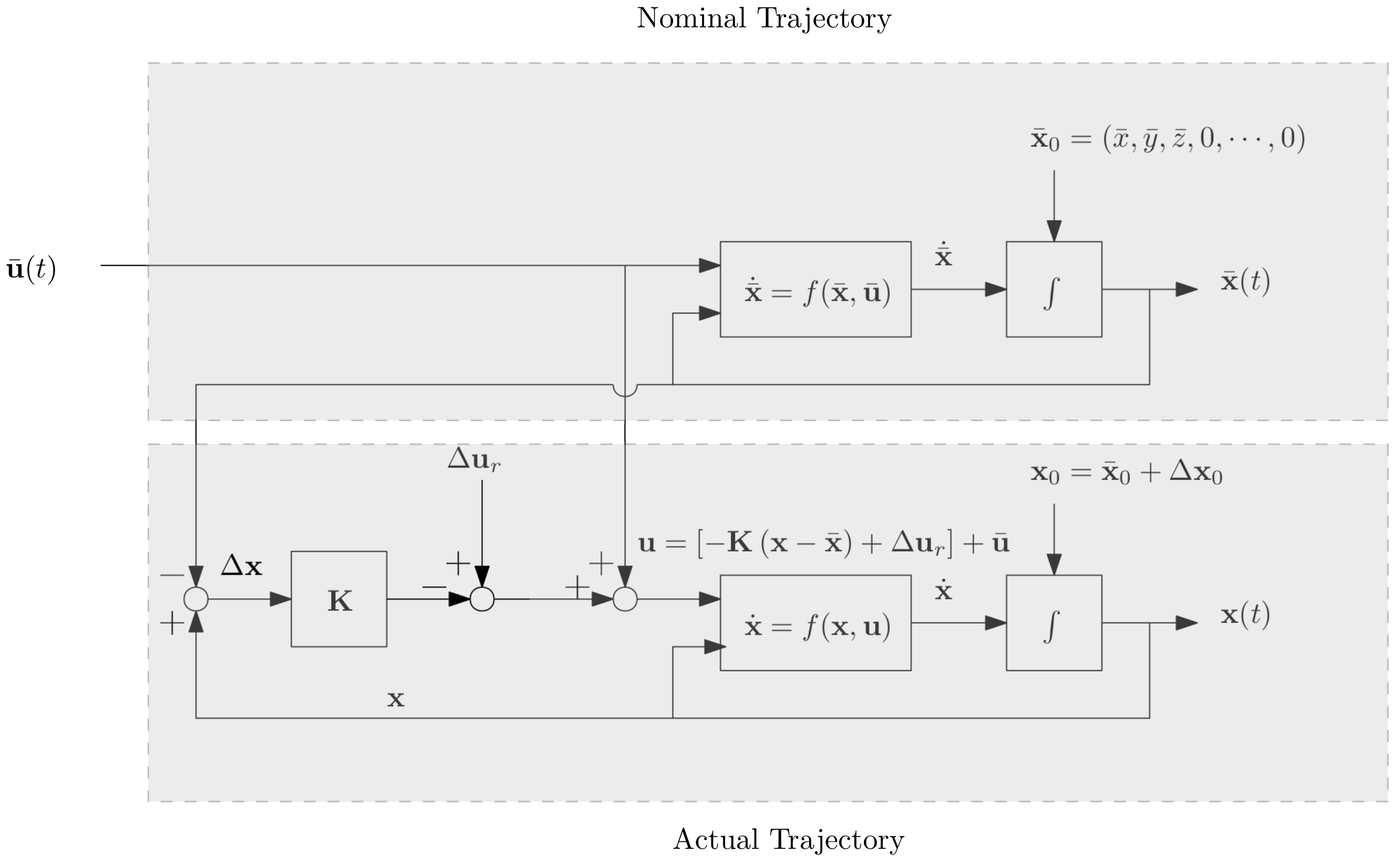
The flow chart for simulations of nonlinear system is presented in Figure 25. The simulations are divided into two parts: one part simulates the nominal trajectory, (i.e., the hovering states in this research); the other part simulates the actual trajectory. The control gain obtained from linearized system is employed in the nonlinear system directly. The state offset is determined by , where the over bar denotes nominal states or nominal control. In this simulation, the hexacopter is to track the nominal trajectory, leading to the reference command .
In the simulations, the initial conditions of the nominal trajectory are set as the hovering state. Without loss of generality, we let . Because the values of do not affect the simulation results, this setting helps to clearly display the propagation of the position offset in the actual response. The differential equations are the original nonlinear EOMs in Equations (A1)–(A12). is the initial condition vector used in the simulations of linearized cases. Moreover, only four of the seven cases are partly controllable. Among the four cases, Case 1 and Case 2 are identical whereas Case 3 and Case 5 are similar. Therefore, we only present the simulations of Case 2 and Case 3 as examples.
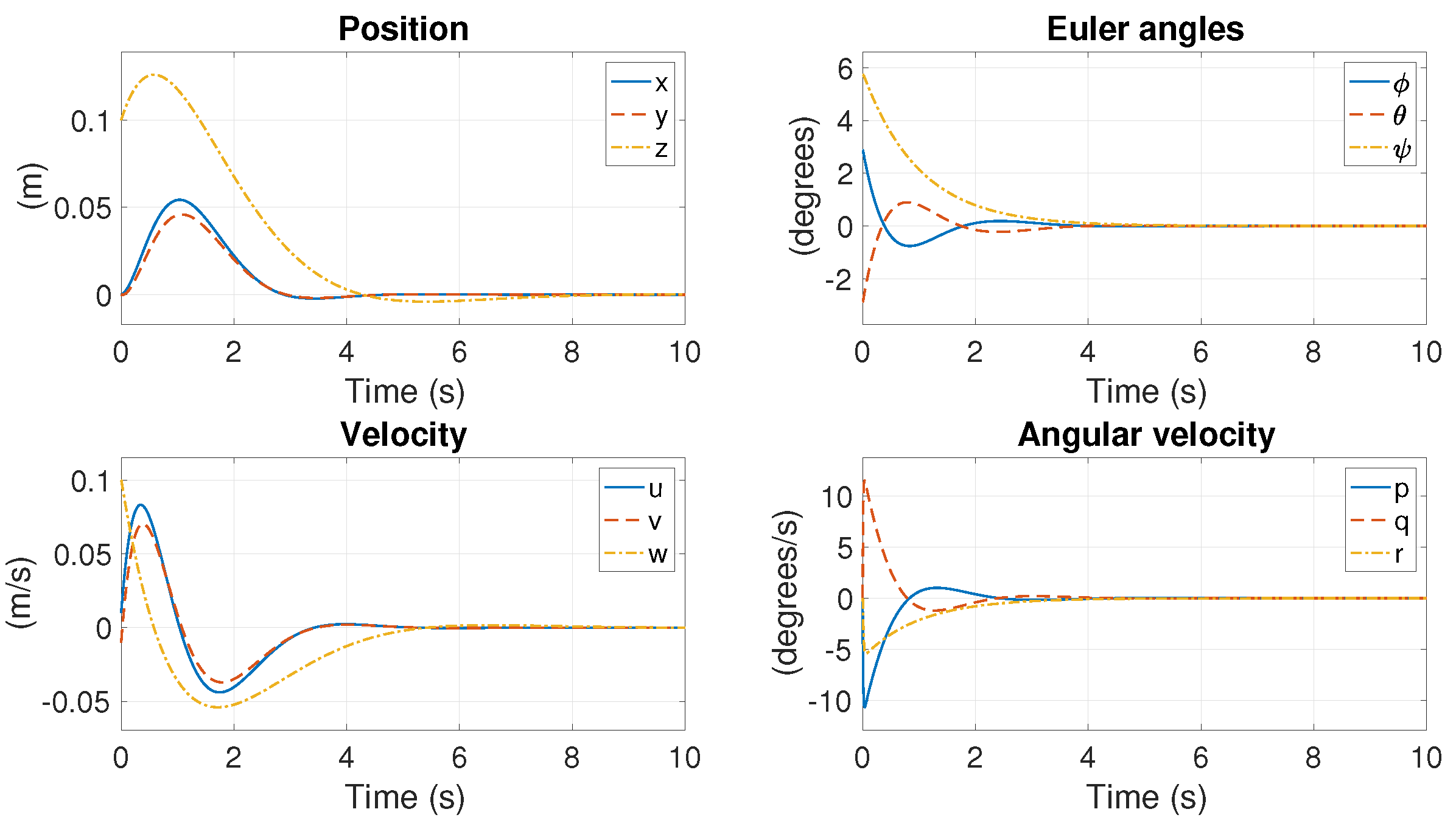
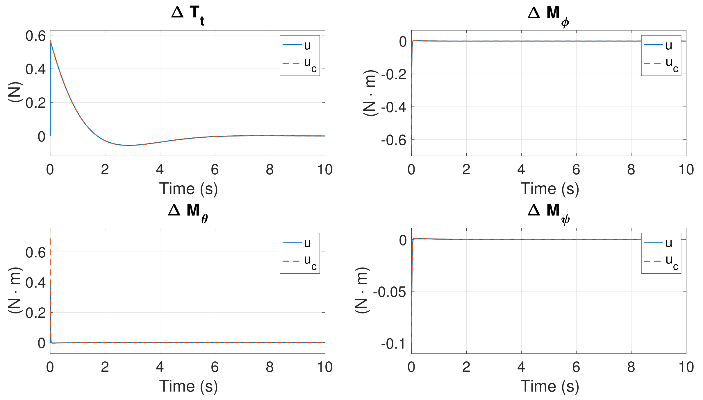
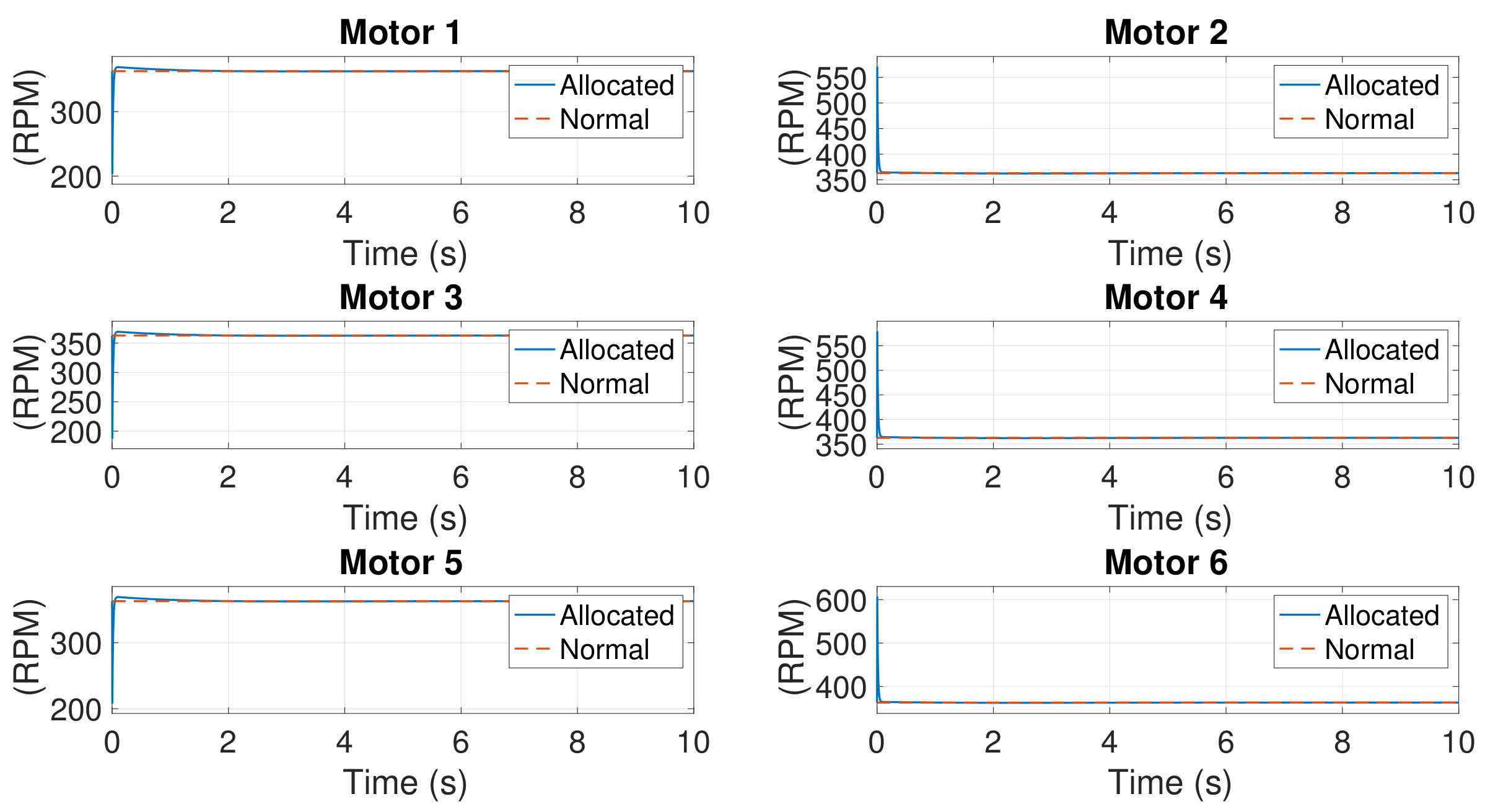
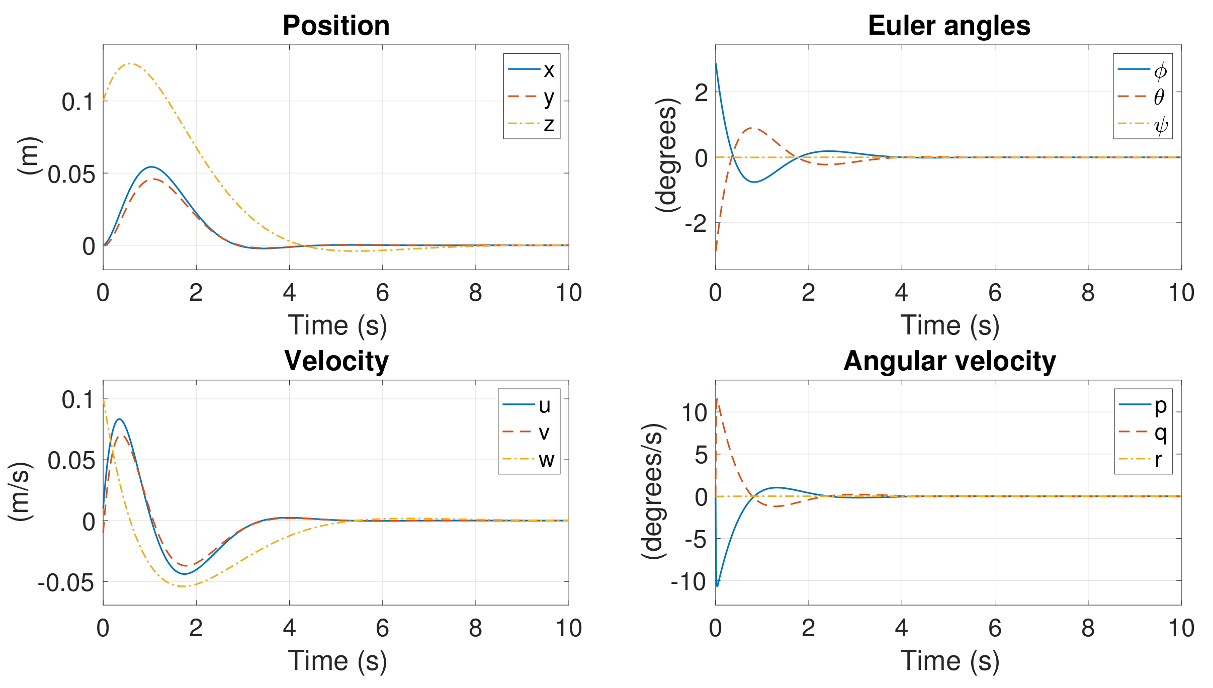
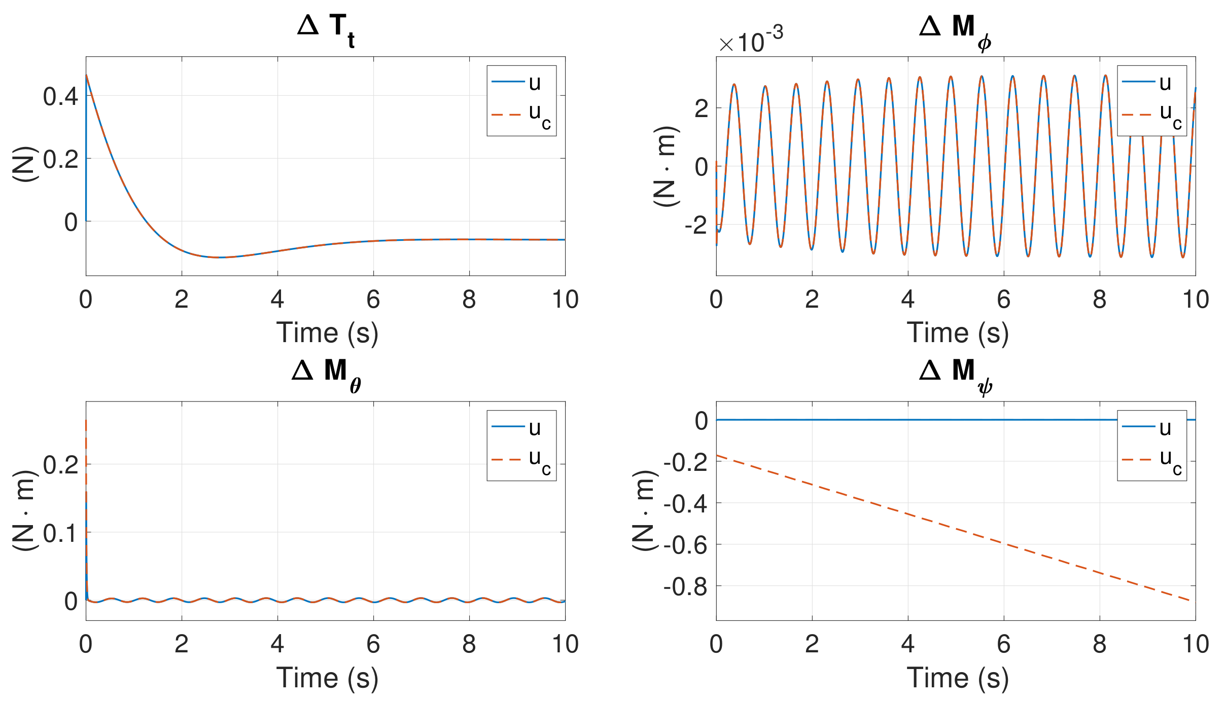
5.7.2. Case 2 as an Example
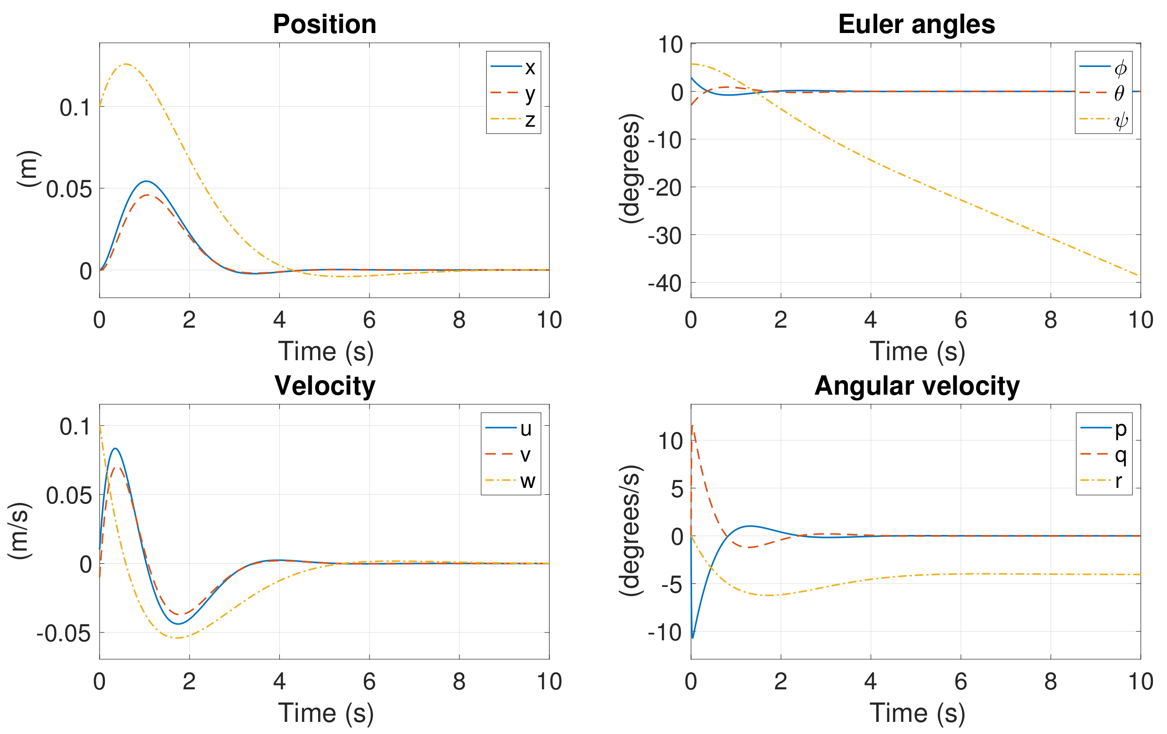
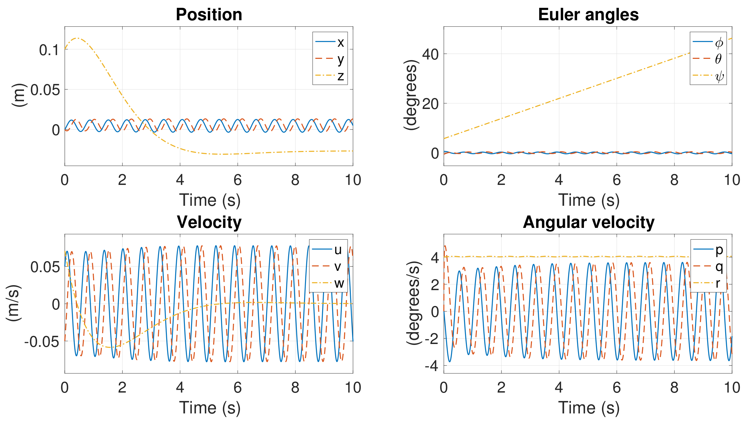
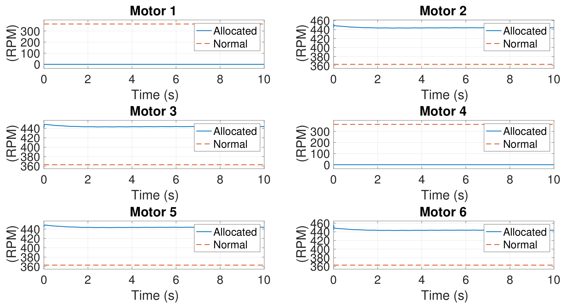
In Section 5.3, remains constant and r converges to zero due to the lack of yawing control. Other states are stabilized and converge to zeros as expected. Figure 26, Figure 27 and Figure 28 present the simulations of nonlinear response under identical initial offset as in Section 5.3.
In the linear level, states are decoupled. Nonconvergence of does not influence other states. In nonlinear level, all states are coupled. To control the position, nonconvergence of causes small oscillation of and , leading to wobbling of the hexacopter. The feedback of wobbling furthermore causes the divergence of gradually, implying that the hexacopter spins. This is different from linear response. Except for uncontrollable yawing motion, other states are controllable, the hexacopter is roughly maneuverable, and it can be landed safely. One can see this phenomena in a real flight video [28].
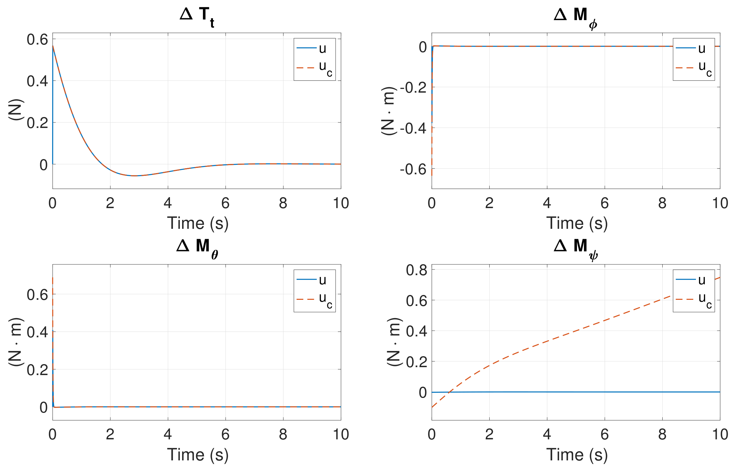
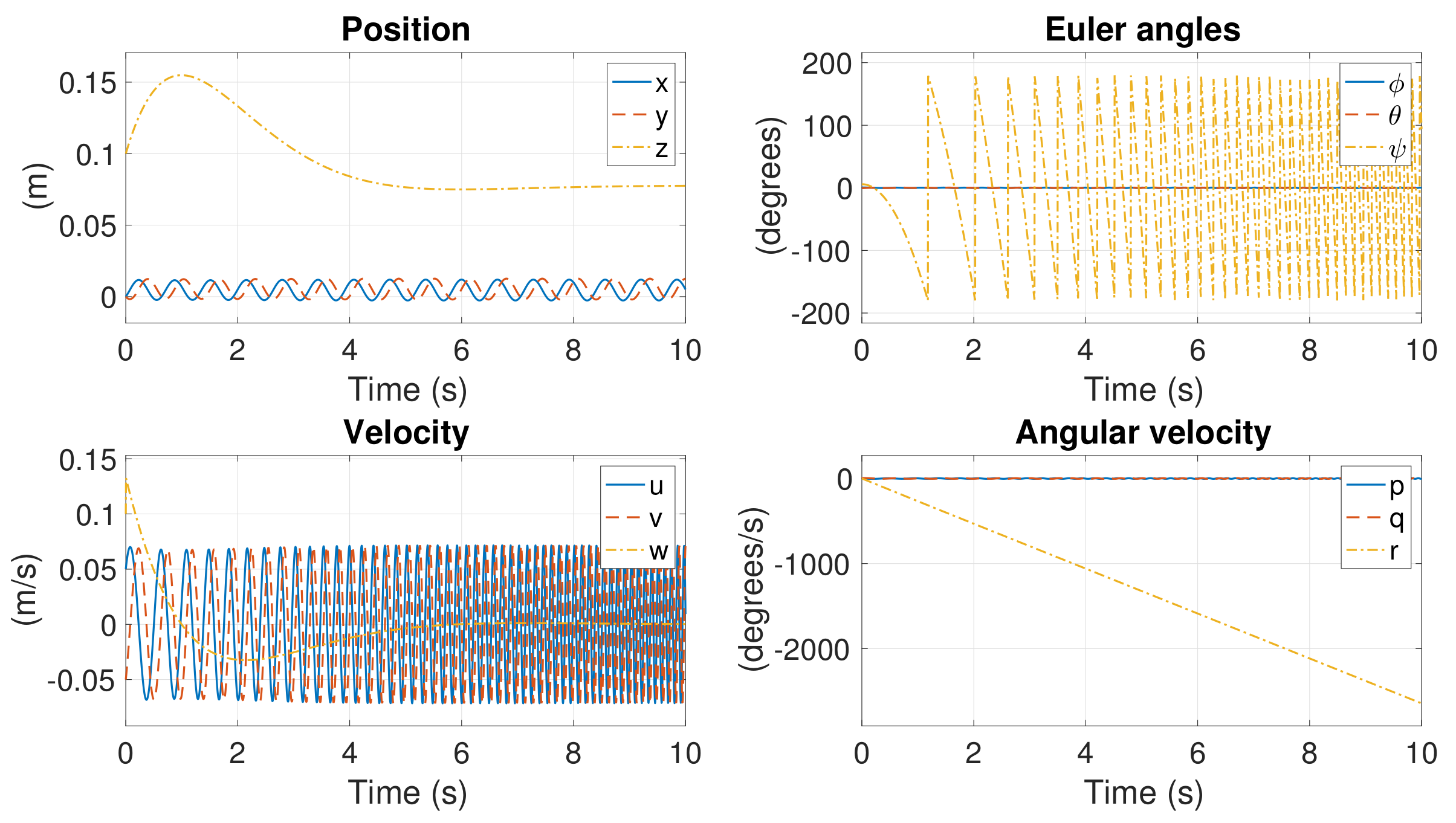
5.7.3. Case 3 as an Example
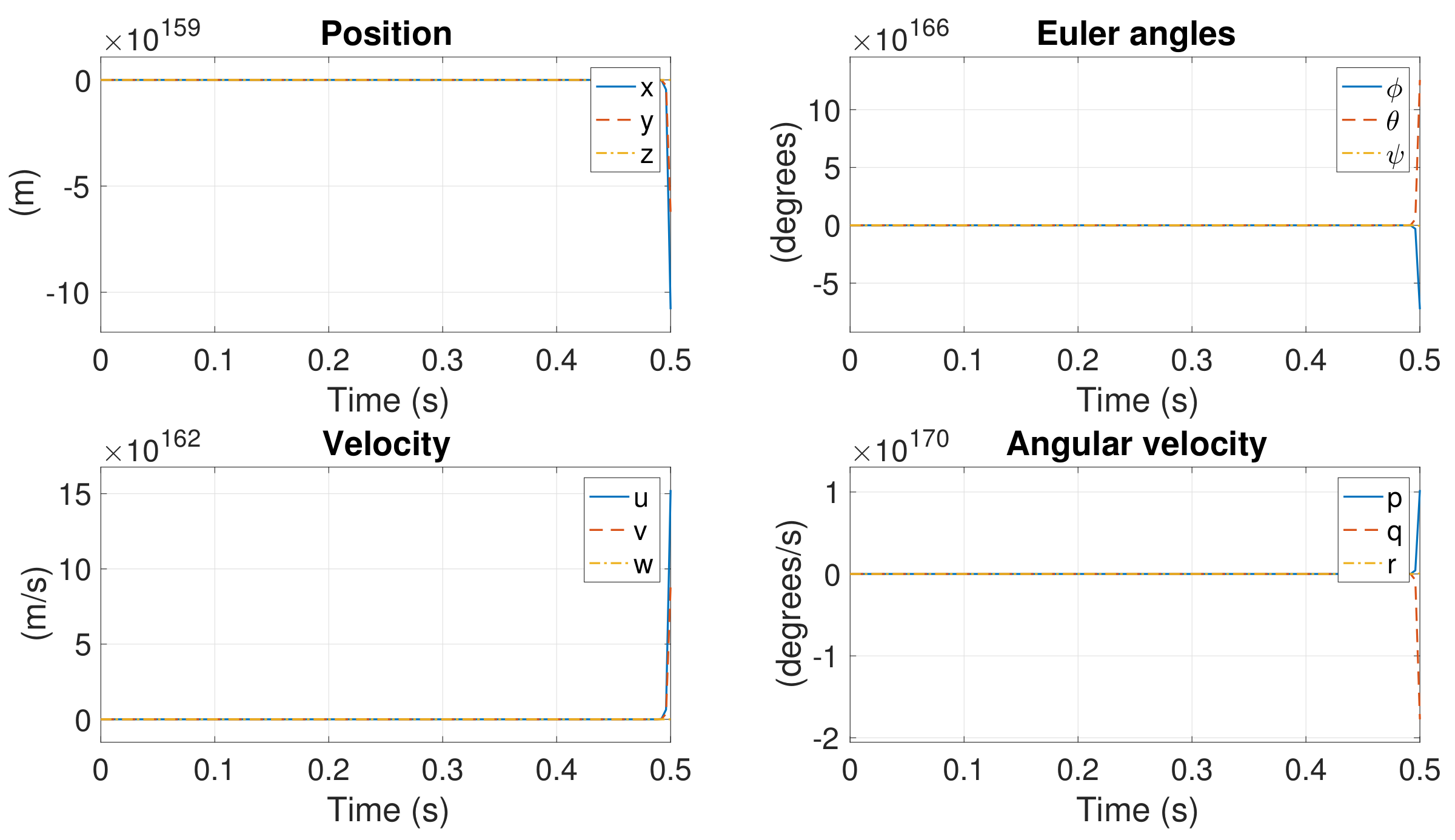
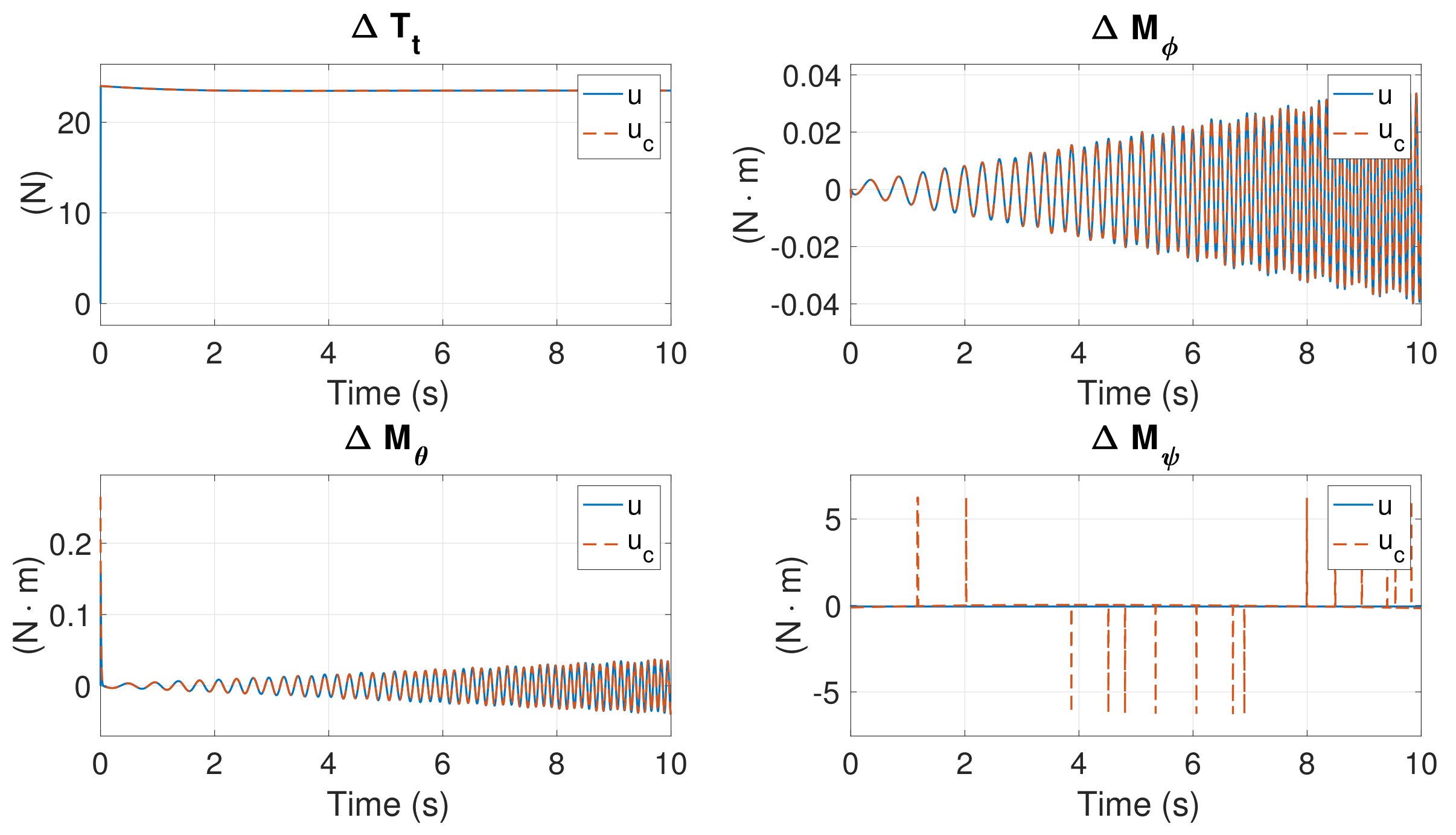
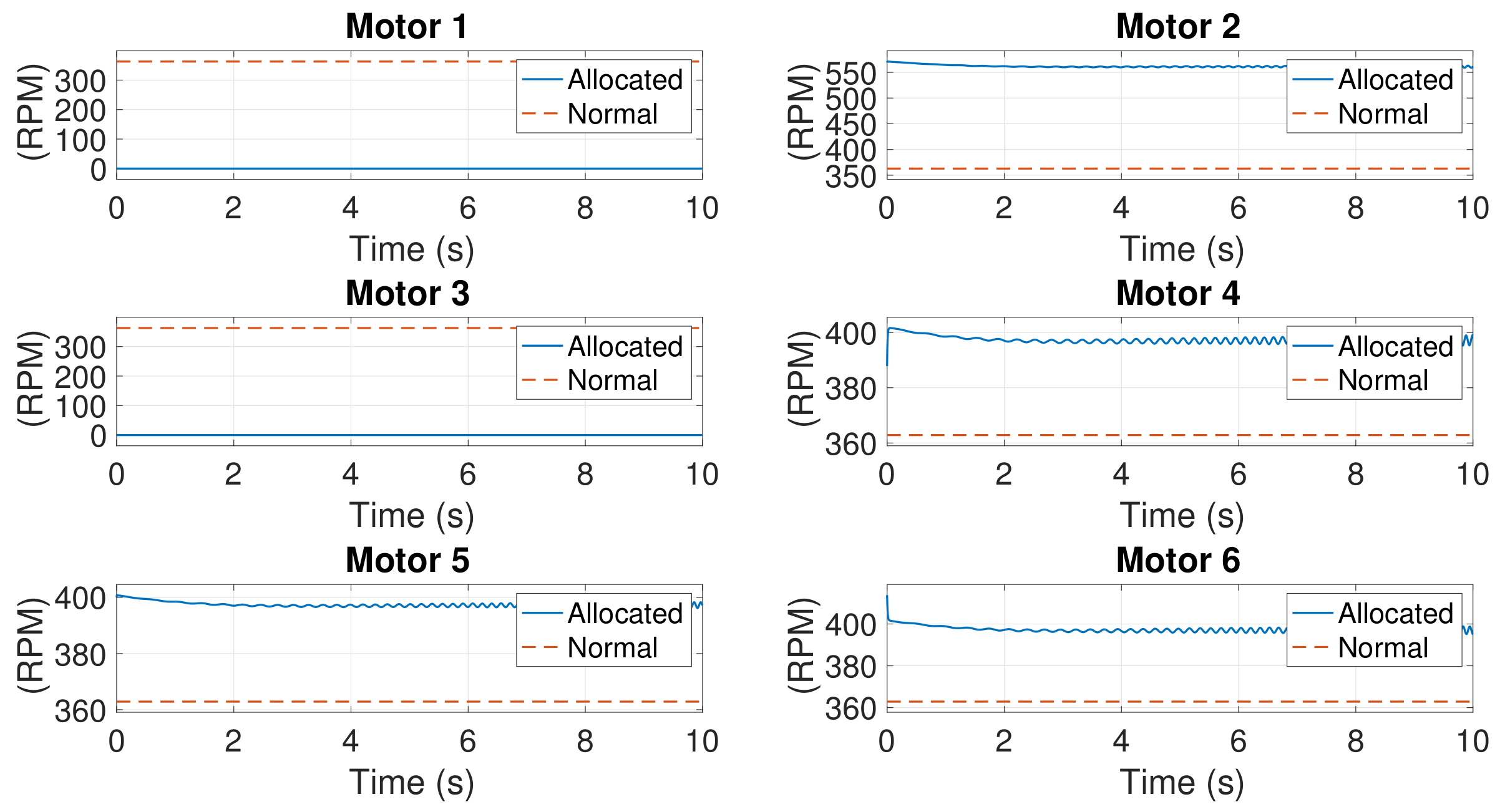
In Section 5.4, diverges very fast due to unbalanced yawing moment. This is the cost for the controllability of other states at the linear level. However, uncontrollable yawing motion at the nonlinear level may cause problems in controlling the whole hexacopter in real flight.
Figure 29, Figure 30 and Figure 31 present the simulations of nonlinear response under identical initial offset as in Section 5.4. From the simulations, one can see that diverges even more severely at the nonlinear level, implying that the hexacopter spins considerably. However, despite small oscillations in the planar motion and some offset in the z-direction, the position of the hexacopter is quite steady. This implies that, by applying our algorithm, the hexacopter must spin sharply, wobble, move around the hovering position, and move slightly higher or lower after Motors #1, #3, and #5 are lost. Although this may appear somewhat scary, the hexacopter is maneuverable and can be landed safely. Perhaps this scenario is too difficult for a human pilot to handle; we did not find any real-flight clips that featured human pilots managing such emergencies.
6. Conclusions and Future Work
6.1. Conclusions
This paper proposes a control allocation algorithm for hexacopters subject to motor failure during flight. More specifically, a hovering hexacopter is considered in the algorithm. The main goal of this paper is to create states that allow the pilot to gain limited control of the hexacopter and perform emergent landing. Potential cases of motor failure include failure of one, two, or three motors, leading to seven scenarios. Failure of more than three motors is uncontrollable, and, hence, out of the scope of this paper. To avoid from change of control or control gain, which may require additional effort during flight, this research solves the motor failure problem by retaining the previous allocation of the control gain but reallocating the rotational speeds. Specifically, the following results are presented: (a) an allocation matrix is proposed to redistribute the control forces so that it is possible to regain (limited) controllability without modifying control gain; (b) seven cases are studied to analyze their respective controllability; (c) numerical simulations in both linearized dynamics and original dynamics also verify the derived results. According to the derivation and simulations, it has been proven that
- the pilot is able to regain controllability of states other than yawing motion when two opposite motors have failed;
- for the case with only one failed motor, the best strategy is to turn off the opposite motor and perform the same maneuver as in the previous scenario;
- for the case with two failed motors with one working motor in between, the pilot is able to regain controllability of states other than yawing motion. In this scenario, however, the hexacopter tends to spin and wobble severely.
- for the case with three failed motors with one working motor in between, the pilot is able to regain controllability of states other than yawing motion. Similar to the previous scenario, the hexacopter tends to spin and wobble severely.
- for other cases, it is very markedly difficult for the pilot to regain controllability and safely land the hexacopter.
6.2. Future Work
At the current stage, this paper focuses on the study of the allocation algorithm and the verification of the algorithm through numerical simulations. In the future, some perspective studies are considered, such as implementation of the algorithm in a hexacopter, development of allocation algorithm in a tilted-rotor craft, generalization of this study to cruise states, and so on.
Author Contributions
Conceptualization, F.-H.W. and J.-K.S.; methodology, F.-H.W., F.-Y.H. and J.-K.S.; software, F.-H.W. and F.-Y.H.; validation, F.-Y.H. and J.-K.S.; formal analysis, F.-H.W. and F.-Y.H.; investigation, F.-H.W.; resources, F.-H.W.; writing—original draft preparation, F.-H.W.; writing—review and editing, F.-Y.H.; supervision, J.-K.S.; project administration, F.-Y.H.; funding acquisition, F.-Y.H. All authors have read and agreed to the published version of the manuscript.
Funding
This research was funded by National Space Organization via funding NSPO-S-109133.
Conflicts of Interest
The authors declare no conflict of interest.
Appendix A. Linearization of Equations of Motion
Expanding Equations (1)–(5) yields the EOMs of the hexacopter. These equations are outlined as follows:
According to linear theory, the linearization is performed by
Moreover, the variations of the air resistant and the yaw counter torque are relatively small during hover. As a result, the two terms are neglected in the linearization. With the aforementioned assumptions, can be detailed as follows:
where
and . Similarly, is detailed as follows:
Let the rotation rates of rotors be the control inputs. Then, and are given by
Let lift force and moments be the control inputs. Then, and are given by
Appendix B. Allocation Matrices
- Case 0:
- Case 1 and Case 2:
- Case 3:
- Case 5:
References
- Lu, P.; van Kampen, E.J. Active fault-tolerant control for quadrotors subjected to a complete rotor failure. In Proceedings of the 2015 IEEE/RSJ International Conference on Intelligent Robots and Systems (IROS), Hamburg, Germany, 28 September–2 October 2015; pp. 4698–4703. [Google Scholar]
- Falconí, G.P.; Holzapfel, F. Adaptive fault tolerant control allocation for a hexacopter system. In Proceedings of the 2016 American Control Conference (ACC), Boston, MA, USA, 6–8 July 2016; pp. 6760–6766. [Google Scholar]
- Choi, B.; Kim, Y. Robust control allocation with adaptive backstepping flight control. Proc. Inst. Mech. Eng. Part G J. Aerosp. Eng. 2013, 228, 1033–1046. [Google Scholar] [CrossRef]
- Mueller, M.W.; D’Andrea, R. Stability and control of a quadrocopter despite the complete loss of one, two, or three propellers. In Proceedings of the 2014 IEEE International Conference on Robotics and Automation (ICRA), Hong Kong, China, 31 May–7 June 2014; pp. 45–52. [Google Scholar]
- Du, G.; Quan, Q.; Cai, K. Additive-state-decomposition-based dynamic inversion stabilized control of a hexacopter subject to unknown propeller damages. In Proceedings of the 32nd Chinese Control Conference, Xi’an, China, 26–28 July 2013; pp. 6231–6236. [Google Scholar]
- Rotondo, D.; Nejjari, F.; Puig, V. Robust quasi-LPV model reference FTC of a quadrotor UAV subject to actuator faults. Int. J. Appl. Math. Comput. Sci. 2015, 25, 7–22. [Google Scholar] [CrossRef] [Green Version]
- Raabe, C.T. Adaptive, Failure-Tolerant Control for Hexacopters. In Proceedings of the AIAA Infotech@Aerospace (I@A) Conference, Boston, MA, USA, 19–22 August 2013. [Google Scholar] [CrossRef]
- Cheon, J.; Kim, C.; Lee, J.; Kwon, S. New Method for Detecting Failures of Power Converter Module in Control Rod Control System. In Proceedings of the 2006 IEEE International Symposium on Industrial Electronics, Montreal, QC, Canada, 9–13 July 2006; Volume 2, pp. 1566–1570. [Google Scholar] [CrossRef]
- Contreras-Medina, L.M.; Romero-Troncoso, R.D.J.; Cabal-Yepez, E.; Rangel-Magdaleno, J.D.J.; Millan-Almaraz, J.R. FPGA-Based Multiple-Channel Vibration Analyzer for Industrial Applications in Induction Motor Failure Detection. IEEE Trans. Instrum. Meas. 2010, 59, 63–72. [Google Scholar] [CrossRef]
- Hasan, A.; Tofterup, V.; Jensen, K. Model-Based Fail-Safe Module for Autonomous Multirotor UAVs with Parachute Systems. In Proceedings of the 2019 International Conference on Unmanned Aircraft Systems (ICUAS), Atlanta, GA, USA, 11–14 June 2019; pp. 406–412. [Google Scholar] [CrossRef]
- Glowacz, A. Fault diagnosis of electric impact drills using thermal imaging. Measurement 2021, 171, 108815. [Google Scholar] [CrossRef]
- Du, G.X.; Quan, Q.; Yang, B.; Cai, K.Y. Controllability Analysis for Multirotor Helicopter Rotor Degradation and Failure. J. Guid. Control. Dyn. 2015, 38, 978–985. [Google Scholar] [CrossRef] [Green Version]
- Mehmood, H.; Nakamura, T.; Johnson, E.N. A maneuverability analysis of a novel hexarotor UAV concept. In Proceedings of the 2016 International Conference on Unmanned Aircraft Systems (ICUAS), Arlington, VA, USA, 7–10 June 2016; pp. 437–446. [Google Scholar] [CrossRef]
- Michieletto, G.; Ryll, M.; Franchi, A. Fundamental Actuation Properties of Multirotors: Force-Moment Decoupling and Fail-Safe Robustness. IEEE Trans. Robot. 2018, 34, 702–715. [Google Scholar] [CrossRef] [Green Version]
- Merheb, A.R.; Noura, H.; Bateman, F. A novel emergency controller for quadrotor UAVs. In Proceedings of the 2014 IEEE Conference on Control Applications (CCA), Juan Les Antibes, France, 8–10 October 2014; pp. 747–752. [Google Scholar]
- Tjønnås, J.; Johansen, T.A. Adaptive control allocation. Automatica 2008, 44, 2754–2765. [Google Scholar] [CrossRef] [Green Version]
- Nagarjuna, K.; Suresh, G.R. Design of effective landing mechanism for fully autonomous Unmanned Aerial Vehicle. In Proceedings of the 2015 3rd International Conference on Signal Processing, Communication and Networking (ICSCN), Chennai, India, 26–28 March 2015; pp. 1–6. [Google Scholar] [CrossRef]
- Wang, B.; Zhang, Y. An Adaptive Fault-Tolerant Sliding Mode Control Allocation Scheme for Multirotor Helicopter Subject to Simultaneous Actuator Faults. IEEE Trans. Ind. Electron. 2018, 65, 4227–4236. [Google Scholar] [CrossRef] [Green Version]
- Lee, S.J.; Jang, I.; Kim, H.J. Fail-Safe Flight of a Fully-Actuated Quadrotor in a Single Motor Failure. IEEE Robot. Autom. Lett. 2020, 5, 6403–6410. [Google Scholar] [CrossRef]
- Bordignon, K.; Bessolo, J. Control allocation for the X-35B. In Proceedings of the 2002 Biennial International Powered Lift Conference and Exhibit, Williamsburg, VA, USA, 5–7 November 2002; p. 6020. [Google Scholar]
- Marks, A.; Whidborne, J.F.; Yamamoto, I. Control allocation for fault tolerant control of a VTOL octorotor. In Proceedings of the 2012 UKACC International Conference on Control, Cardiff, UK, 3–5 September 2012; pp. 357–362. [Google Scholar] [CrossRef]
- Nelson, R. Flight Stability and Automatic Control, 2nd ed.; McGraw-Hill Education: New York, NY, USA, 1997. [Google Scholar]
- Fogelberg, J. Navigation and Autonomous Control of a Hexacopter in Indoor Environments. Master’s Thesis, Lund University, Lund, Sweden, 2013. [Google Scholar]
- Leishman, R.C.; Macdonald, J.C.; Beard, R.W.; McLain, T.W. Quadrotors and Accelerometers: State Estimation with an Improved Dynamic Model. IEEE Control. Syst. Mag. 2014, 34, 28–41. [Google Scholar]
- Martin, P.; Salaün, E. The true role of accelerometer feedback in quadrotor control. In Proceedings of the 2010 IEEE International Conference on Robotics and Automation, Anchorage, AK, USA, 3–7 May 2010; pp. 1623–1629. [Google Scholar]
- Chang, C.W.; Shiau, J.K. Quadrotor formation strategies based on distributed consensus and model predictive controls. Appl. Sci. 2018, 8, 2246. [Google Scholar] [CrossRef] [Green Version]
- Lancaster, P.; Rodman, L. Algebraic Riccati Equations; Oxford University Press: Oxford, UK, 2002; p. 504. [Google Scholar]
- Pospisil, J. Hexacopter Motor Fail (Youtube Video). 2013. Available online: https://www.youtube.com/watch?v=ZeHI2p6mjNM (accessed on 30 April 2013).
Figure 1.
Block diagram of motor failure.

Figure 2.
Coordinate system of the hexacopter and the numbering of rotors. The diagram schematizes the top view.
Figure 2.
Coordinate system of the hexacopter and the numbering of rotors. The diagram schematizes the top view.

Figure 3.
Control allocation architecture.

Figure 4.
Control allocation between the command given by controller and the system.

Figure 5.
Failure states of a six-motor system.

Figure 6.
State responses in Case 0.

Figure 7.
Control inputs in Case 0.

Figure 8.
Rotational speeds of motors in Case 0.

Figure 9.
Position response in Case 1.

Figure 10.
Control inputs in Case 1.

Figure 11.
Rotational speeds of motors in Case 1.

Figure 12.
Position response in Case 1 with controllable initial conditions.

Figure 13.
Control responses in Case 1 with controllable initial conditions.

Figure 14.
Rotational speeds of motors in Case 1 with controllable initial conditions.

Figure 15.
Position response in Case 3.

Figure 16.
Control inputs in Case 3.

Figure 17.
Rotational speeds of motors in Case 3.

Figure 18.
Position responses in Case 4.

Figure 19.
Position response in Case 5.

Figure 20.
Control inputs in Case 5.

Figure 21.
Rotational speeds of rotors in Case 5.

Figure 22.
Position response in Case 5 with controllable initial condition.

Figure 23.
Control response in Case 5 with controllable initial condition.

Figure 24.
Rotational speeds of motors in Case 5 with controllable initial conditions.

Figure 25.
Flowchart for simulations of original nonlinear system.

Figure 26.
Nonlinear position response in Case 2.

Figure 27.
Control inputs response in Case 2.

Figure 28.
Rotational speeds of motors response in Case 2.

Figure 29.
Nonlinear position response in Case 3.

Figure 30.
Nonlinear control inputs in Case 3.

Figure 31.
Nonlinear rotational speeds of motors in Case 3.


Table 1.
Simulation parameters of the hexacopter.
| Parameters | Values | Units | Parameters | Values | Units |
|---|---|---|---|---|---|
| g | |||||
| m | kg | ||||
| l | m | ||||
| d | b |
Publisher’s Note: MDPI stays neutral with regard to jurisdictional claims in published maps and institutional affiliations. |
© 2021 by the authors. Licensee MDPI, Basel, Switzerland. This article is an open access article distributed under the terms and conditions of the Creative Commons Attribution (CC BY) license (http://creativecommons.org/licenses/by/4.0/).
Share and Cite
MDPI and ACS Style
Wen, F.-H.; Hsiao, F.-Y.; Shiau, J.-K. Analysis and Management of Motor Failures of Hexacopter in Hover. Actuators 2021, 10, 48. https://0-doi-org.brum.beds.ac.uk/10.3390/act10030048
AMA Style
Wen F-H, Hsiao F-Y, Shiau J-K. Analysis and Management of Motor Failures of Hexacopter in Hover. Actuators. 2021; 10(3):48. https://0-doi-org.brum.beds.ac.uk/10.3390/act10030048
Chicago/Turabian StyleWen, Fu-Hsuan, Fu-Yuen Hsiao, and Jaw-Kuen Shiau. 2021. "Analysis and Management of Motor Failures of Hexacopter in Hover" Actuators 10, no. 3: 48. https://0-doi-org.brum.beds.ac.uk/10.3390/act10030048
Note that from the first issue of 2016, this journal uses article numbers instead of page numbers. See further details here.