
Mono-Vision Based Lateral Localization System of Low-Cost Autonomous Vehicles Using Deep Learning Curb Detection

School of Automotive Studies, Tongji University, Shanghai 200092, China
*
Author to whom correspondence should be addressed.
Actuators 2021, 10(3), 57; https://0-doi-org.brum.beds.ac.uk/10.3390/act10030057
Submission received: 21 January 2021
/
Revised: 4 March 2021
/
Accepted: 8 March 2021
/
Published: 11 March 2021
(This article belongs to the Special Issue Actuators for Intelligent Electric Vehicles)
Abstract
:The localization system of low-cost autonomous vehicles such as autonomous sweeper requires a highly lateral localization accuracy as the vehicle needs to keep a near lateral-distance between the side brush system and the road curb. Existing methods usually rely on a global navigation satellite system that often loses signal in a cluttered environment such as sweeping streets between high buildings and trees. In a GPS-denied environment, map-based methods are often used such as visual and LiDAR odometry systems. Apart from heavy computation costs from feature extractions, they are too expensive to meet the low-price market of the low-cost autonomous vehicles. To address these issues, we propose a mono-vision based lateral localization system of an autonomous sweeper. Our system relies on a fish-eye camera and precisely detects road curbs with a deep curb detection network. Curbs locations are then referred to as straightforward marks to control the lateral motion of the vehicle. With our self-recorded dataset, our curb detection network achieves 93% pixel-level precision. In addition, experiments are performed with an intelligent sweeper to prove the accuracy and robustness of our proposed approach. Results demonstrate that the average lateral distance error and the maximum invalid rate are within 0.035 m and 9.2%, respectively.
1. Introduction
Over the few years, autonomous vehicles have gained a lot of attention and witnessed remarkable progress. Companies such as Google and Tesla have the same goal toward fully L5 self-driving cars although they differ in approach from a design and engineering philosophy. Despite great success achieved by these companies, it will still take a rather long time before autonomous cars are widespread on the public roads in any weather and under any condition. As a result, there are a bunch of universities and companies concentrating on developing low-speed and low-cost autonomous vehicles that run in a limited, tightly controlled environment.
Among all the fundamental components (e.g., perception, decision-making, motion planning and localization) in the field of autonomous vehicle, localization is one of the most important and challenging problems. There are always inevitable contradictions of the highly precise localization systems and low-cost hardware requirements, especially for a low-cost autonomous vehicle such as a sweeper.
The easiest way to obtain the location of vehicles is using a global navigation satellite system (GNSS) with an inertial navigation system (INS), which is widely used for autonomous vehicles running in an open area such as on a highway [1,2]. The drawbacks are obvious. Firstly, the cost of a highly accurate GNSS/INS system is almost of equal value to a low-cost vehicle, which is certainly unacceptable. In addition, in a cluttered environment such as streets inside high buildings and trees, or in a GPS-denied environment such as a parking garage, GNSS signals are not feasible. To overcome this problem, several map-based methods are developed, where the features extracted from the environments using LiDARs, cameras, or other sensors are matched to the HD digital map to aid localization [3,4,5,6,7,8,9,10,11]. Apart from heavy computation costs from feature extraction and data association, they are too expensive to meet the low-price requirements of the low-cost autonomous vehicles.
To address these issues, we propose a fish-eye mono-vision based lateral localization system of an autonomous sweeper, which is highly efficient, low cost, and less complex compared to existing solutions. The framework is illustrated in Figure 1. Our system relies on a monocular fish-eye camera and precisely detects the road curbs with our proposed deep learning model. Curb locations are then referred as straightforward marks to control the lateral motion of the autonomous vehicle. At the heart of our work, we propose a deep curb detection network which serves as a key component to ensure a near lateral-distance (e.g., 0.2 m) between the side brush system and the sweeping road curb.
It is worth noting that, although curb detection is a traditional problem in the field of autonomous vehicles [12,13,14,15,16], most of the existing works utilize a front-facing camera or 3D LiDAR to detect curbs and search the road boundary, and further segment the travelable regions. They differ from our work in three aspects. Firstly, we are using a fish-eye side-facing camera to detect the road curbs while they often use a front-facing camera to detect curbs and lanes to segment the travelable region. Secondly, travelable region segmentation requires a pretty-low accuracy of curb detection as vehicles are often far away from the road boundary. Thirdly, for the expensive LiDAR-based method or stereo camera-based method, curbs are often detected based on strong assumptions such as the height of road curbs. These methods are generally not applicable to detect the curbs without obvious geometric features.
In contrast, our deep curb detection network is designed for a high-precision localization system of an autonomous sweeper. Our network consists of three key modules: a road scene classification module acts as the pre-processing procedure to classify the images as Scene with Obstacles, Scene with Curbs or Scene with Intersection. A curb region of interest (CRoI) module is utilized to obtain the curb region of interest. Subsequently, a semantic segmentation module is developed to accurately segment the curbs in CRoI. We combined U-Net [17] and SCNN [18] into our model. U-Net has an excellent performance in semantic segmentation problems and the slice-by-slice convolution in SCNN helps to make better use of spatial information. We evaluate our deep curb detection with a self-recorded dataset and achieve 93% pixel-level precision. Apart from offline experiments, we also perform online experiments on the autonomous sweeper developed at Tongji University, and compare our mono-vision based lateral localization system with the LiDAR-based localization system. The experiment results demonstrate that the average lateral distance error and the maximum invalid rate are within 0.035 m and 9.2%, respectively, and thus our system gets a better performance in terms of the robustness of the localization system compared to the LiDAR-based method.
The main contributions of this work are as follows:
- A mono-vision based lateral localization system of a low-cost autonomous vehicle is developed. Our system relies on a monocular fish-eye camera that is much cheaper than LiDARs.
- A CRoI module is proposed to obtain the curb region of interest to crop the image for the following semantic segmentation module, which improves the efficiency of the proposed method.
- We propose a novel semantic segmentation module based on the combination of U-Net and SCNN.
2. Related Works
The localization system is one of the most important components in the autonomous vehicle. Many efforts have been invested in this research topic. One of the most common solutions is using GNSS/INS. However, the accuracy of the traditional GNSS/INS method cannot meet the requirements of autonomous vehicles in cluttered environments and GPS-denied scenarios. To improve accuracy and robustness of localization, several map-based methods are proposed. For example, in [6], vertical corner features are extracted from the scan data of 3D LiDAR and then matched to pre-built corner map to correct the vehicle position. Similarly, the framework proposed in [5] adopts semantic and distinctive physical objects such as trees, traffic signs, or street lamps as landmarks and the vehicle pose is obtained via the combination of these features and an offline map.
Except for the global localization, lateral localization is also a research focus because of its remarkable assistance for localization. In [7], lateral and orientation information of lane markings is extracted from a video camera to enhance lateral localization accuracy. In [8], two lateral cameras are used to detect road markings and provide the lateral distance between the vehicle and the road borders for lane change. In addition, the information from the camera is combined with a digital map of the road markings to aid the localization from GNSS/INS. In [9], an algorithm which produces the distance of the vehicle to the left and right boundaries of the road-lane is presented. Then, the detected lane-markings are used as measurements for a Bayes filter to obtain the lateral position of the vehicle.
In addition to lane markings, road curb is another important feature for the improvement of lateral localization. In [10], a curb detection algorithm using 3D-LiDAR is performed, and the detection result matches the high-precision map. Then, the map matching result is fused with the localization of GPS and INS via a Kalman filter. In [13], the point cloud data from a 3D-LiDAR sensor are processed to distinguish on-road and off-road areas. A subsequent sliding-beam method can segment the road, then the position of curbs is obtained via a search-based method for each road segment. In [11], curb detection results obtained from a 3D LiDAR are adopted to correct the lateral errors in localization from GNSS/IMU/DMI(Distance Measuring Instruments). In [19], a deep learning-based method is used to detect visible curbs and occluded curbs. In [20], a Conditional Random Field (CRF) is used to assign the 3D points measured by stereo camera to different parts of a 3D environment model in order to reconstruct the surfaces and in particular the curb. In [21], an ultrasonic sensor-based method is proposed for curb detection. However, the detection method has requirements for the height of the curb and can not perform detection on curbs with low height.
Different from the works mentioned above, a fish-eye mono-vision based lateral localization system of an autonomous sweeper is developed in this paper, which is highly efficient, low cost, and less complex compared to existing solutions. Our system relies on a monocular fish-eye camera and precisely detects the road curbs with our proposed deep learning model. Curb locations are then referred to as straightforward marks to control the lateral motion of the autonomous vehicle.
3. Mono-Vision Based Lateral Localization System
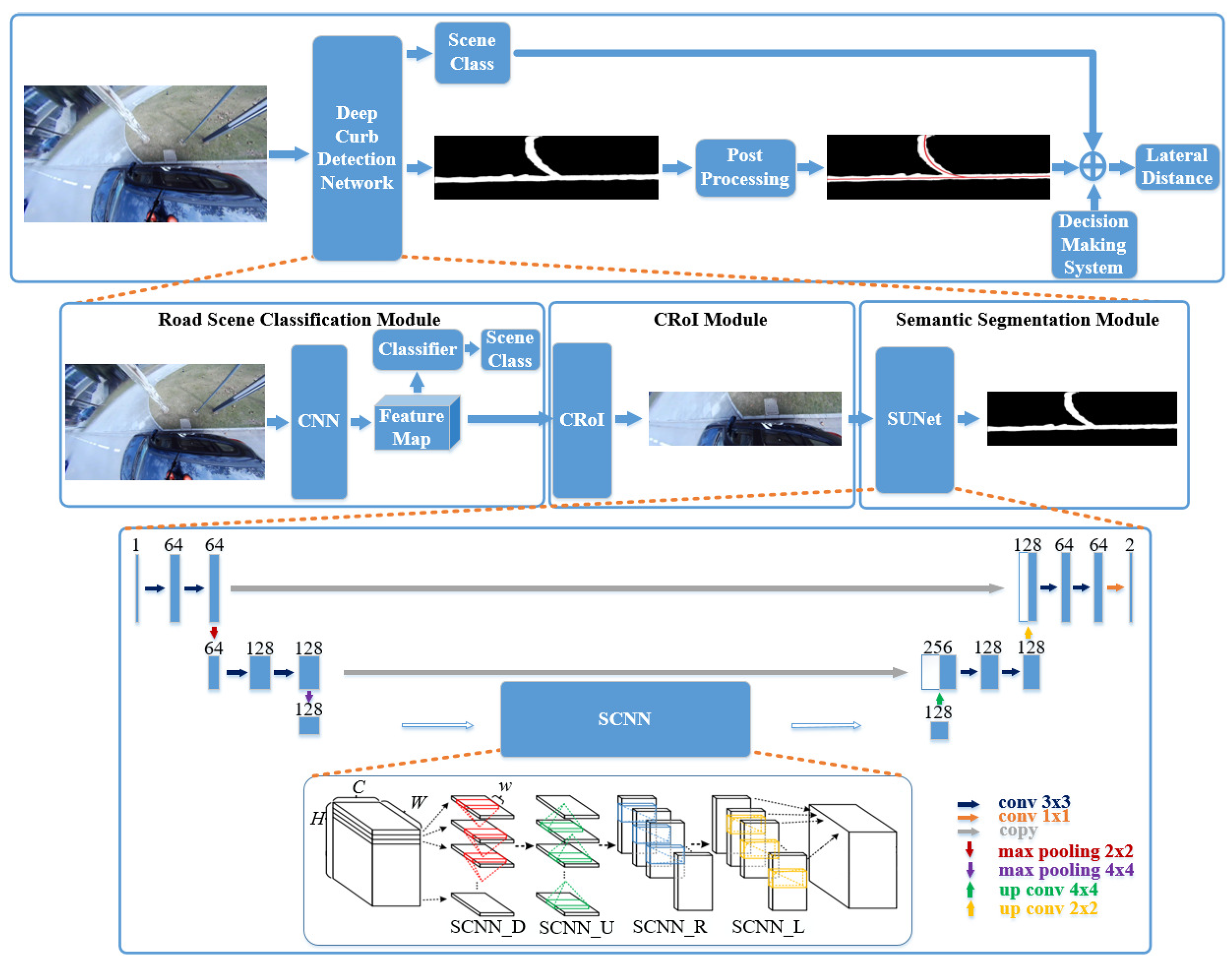
In this work, a fish-eye mono-vision based lateral localization system of a low-cost autonomous vehicle is proposed. A hierarchical structure of the framework is shown in Figure 1. The upper layer of our framework (the first row of Figure 1) depicts the overall work-flow of the lateral localization system. Depending on the curb detection results, the vehicle calculates the lateral distance between itself and the nearest road curb, which is then sent to the vehicle control system. The middle layer of our framework (the second row of Figure 1) is the core component of our system which is a deep curb detection network. It consists of three important modules: road scene classification module, curb region of interest module, and semantic segmentation module. The road scene classification module classifies the road scenes into three classes: Scene with Obstacles, Scene with Curbs and Scene with Intersection. The CRoI module detects the interested region of curbs. As the input image of the semantic segmentation module shrinks, it improves the following semantic segmentation module’s efficiency. Our semantic segmentation module is built based on U-Net [17] and SCNN [18].
The overall lateral localization system is described in Algorithm 1. A road scene image recorded by our side-facing fish-eye camera is firstly entered into our system. The road scene classification module outputs the class label. In the case of the label Scene with Obstacles, there will be no further processing procedure such as semantic segmentation. An obstacle encountering message is transmitted to the decision-making system of the autonomous vehicle. In the case of the label Scene with Curbs and Scene with Intersection, the CRoI is firstly detected, and then a precise segmentation result of the CRoI is obtained. The road curbs’ locations are extracted from the segmentation results. For the road scene classified as Scene with Curbs, a curve is fitted based on the curbs’ locations. For the road scenes classified as Scene with Intersection, there are three possibilities: (1) if the vehicle goes forward, then we fit a straight line with curbs; (2) if the vehicle turns right, then we fit a right-turn curve with curbs; (3) if the vehicle turns left, the localization will be based on the low-cost GPS and the lateral localization accuracy will be less important in this case.
4. Deep Curb Detection Network
In this section, we describe the deep curb detection network which is the core component of the proposed mono-vision based lateral localization system. It consists of three modules: road scene classification module, CRoI module, and semantic segmentation module.
| Algorithm 1 Lateral localization system |
Require: road scene image 1: Enter the image into curb detection network, obtain the and segmentation results; 2: if is then 3: Transmit an obstacle encountering message to the decision-making system of the vehicle; 4: else if is then 5: Fit a curve based on the curbs’ locations; 6: else if is then 7: The decision-making system decide to go forward or turn right; 8: if The vehicle goes forward then 9: Fit a straight line; 10: else if The vehicle turns right then 11: Fit a right-turn curve; 12: else The vehicle turns left 13: Use low-cost GPS for localization. 14: end if 15: end if |
4.1. Road Scene Classification
The road scene classification model acts as a pre-processing procedure of the lateral localization system. It also serves as a basic module for the following CRoI module and semantic segmentation module. We annotate each road scene image recorded by the side-facing fish-eye camera with three labels as Scene with Obstacles, Scene with Curbs and Scene with Intersection (see Figure 2). The road scene classification model is implemented with a pre-trained convolutional neural network VGG-16 [22]. The feature map generated by the VGG-16 model is also passed to the CRoI module. The classified road scene is not only used by the lateral localization system but also transmitted to the motion planning system of the autonomous vehicle.
4.2. CRoI
As shown in Figure 2, curbs only occupy a long and narrow region of the full road scene pictures. To speed up the semantic segmentation module, we decide to detect the curb region of interests (CRoI) before further processing. Inspired by the region proposals widely used by object detection networks [23,24,25], we develop our CRoI module based on region proposal networks (RPN) introduced in Faster-RCNN [25]. The difference between our CRoI module and other RPN networks is that our CRoI module only needs to generate one curb region proposal that is fast and effective. It is worth noting that the road scene classification module is different from the classification step in Fast-RCNN. The latter cannot substitute the former because the road scene classification module we utilize in this work pays more attention to the global description of a road scene image. Additionally, the VGG-16 model used in the road scene classification module shares the same feature map with the RPN network in the CRoI module to avoid redundant computations. As illustrated in the second row of Figure 1, following the pre-trained CNN, there are two parallel branches: feature map to road scene classifier and to the CRoI module.
4.3. Semantic Segmentation
The semantic segmentation module is designed to precisely segment curbs from the CRoI module. We propose our SUNet segmentation model that is a combination of the U-Net [17] and SCNN [18]. The structure of the SUNet can be seen in the third row of Figure 1. Thanks to the contracting path between high resolution features and the upsampled output in U-Net, the successive convolution layer can get both information with a large receptive field from deeper layers and detailed information from the shallower layer. Consequently, U-Net has shown excellent performance in semantic segmentation problems. Therefore, we choose it as the backbone of our semantic segmentation module. The depth of the original U-Net is reduced to reduce the computational complexity.
As mentioned above, a curb is generally a long and narrow structure. The appearance clues are relatively less and the curbs are often interrupted and occluded. Fortunately, the curb is a highly structured feature and a strong spatial relationship exists between curb pixels. Intuitively, if the spatial information of curb can be better utilized, the algorithm should achieve better performance. Based on the above considerations, we adopt the SCNN structure, which is proposed in [18]. In the SCNN structure, traditional layer-by-layer convolutions are replaced by slice-by-slice convolutions within feature maps. As shown in the third row in Figure 1, SCNN_D, SCNN_U, SCNN_R, and SCNN_L represent four directions that slice-by-slice convolutions are applied: downward, upward, rightward, leftward. For instance, in SCNN_D, the feature map with size is split into H slices. The first slice is sent into a convolution layer with kernels of size , and the output is added to the next slice to generate a new slice. This process continues until the bottom slice. The processing procedure of other modules can be learned by analogy. Consequently, the spatial information can be propagated across rows and columns in a layer so that the structure is particularly suitable for structured objects like curbs. As mentioned in [18], SCNN can be flexibly applied to any place of a network. Generally, it should be added after a layer that contains richer information. Thus, we choose to apply SCNN at the bottom of U-Net. It is found that the computational efficiency of SCNN is highly dependent on the size of its input layer. In order to reduce computing time, a max pooling layer is added before the SCNN to reduce the size of the input layer.
5. Experiments
This section describes the details and results of experiments of our mono-vision based lateral localization system. The experiments are divided into two parts, offline experiments with the self-recorded dataset and online experiments with an autonomous sweeper. We evaluate the performance of our deep curb detection network with offline experiments. The localization accuracy and robustness are evaluated with an autonomous sweeper developed at Tongji University.
5.1. Deep Curb Detection Network Implementations
5.1.1. Road Scene Classification and Curb Region of Interest
The road scene classification module is implemented with a pre-trained convolutional neural network VGG-16. Firstly, pre-trained VGG-16 has a restriction of the input image’s size and the original designed image size is . However, the resolution of the fish-eye camera is , so the images in our data set must be resized to fit the requirement of VGG-16. We resize the image to ; in addition, this process would not change the height-width ratio of the raw image. In addition, the resizing is a trade-off to achieve a balance between the resolution and the memory usage of GPU.
Secondly, the CNN of our network is composed of the first 30 layers of VGG-16, and the FC (fully connected) layer is discarded temporarily. When it comes to the classification module, the FC layer is implemented again; however, because of the resize process, dimensions of the tensor here should be handled with care. In contrast to the original VGG-16, the dimension of FC layer is . In addition, the RPN is adopted from Faster-RCNN [25].
In the train procedure, the initial learning rate is set to 0.001 and the learning rate is decayed by a factor of 0.1 every 10 epochs. We adapt cross-entropy loss as the classification loss, and it is incorporated with the losses in RPN. Except for the 30 frozen layers of VGG-16, all of the new layers of the model are initialized from a zero-mean Gaussian distribution with a standard deviation of 0.01. Since the road scene classification module and curb region of interest module share the same feature map, the networks of these modules are trained simultaneously.
5.1.2. Semantic Segmentation
Since the input image is downsampled and upsampled several times in the semantic segmentation network, in order to ensure the consistency of the input and output image size, we extend the size of irregular CRoI that is generated by the CRoI module to the power of 2, such as .
In the training procedure, the initial learning rate is set to 0.001 and decayed by 0.9 every epoch. We also adopt cross-entropy loss as the loss function here. In addition, due to the imbalance of the number of pixels between background and curbs, we set the weight of the loss to be 0.8 for curbs and 0.2 for the background.
The whole network is trained and validated on an Nvidia GTX 1080Ti GPU (NVIDIA Corporation, Santa Clara, CA, USA) and implemented using PyTorch [26].
5.2. Offline Experiments
5.2.1. Dataset
To evaluate the performance of our deep curb detection network, we establish the first-ever road curb detection dataset dedicated to a lateral localization system of a low-speed autonomous vehicle. We use a fish-eye camera with a angle of view. The resolution of the fish-eye camera is . The camera is mounted on the right side of the vehicle, and is facing to the right side of the road. In total, our dataset has 7000 images that are recorded at different locations during daytime, which is very challenging. Regarding the annotation, each image has three labels. The first one is the class of the road scene. The second label is a rectangle of the ground truth of the CRoI. The third label is a fitting curve of the curb in the road scene, which results in a pixel-level mask annotation of the curb.
5.2.2. Experimental Results
We evaluate three modules of our deep curb detection network separately with a self-recorded dataset. We consider the road scene classification module as a three-class classification problem. The classification accuracy with our dataset is 96.5%. For the CRoI module, we adopt average precision (AP) to evaluate the model; it is expressed as:
where represents recall, p denote precision, AP is the area between precision–recall curve and axis, thus , but to simplify the computation, we set , so we replace the integration with a sum of . On a validation set, the AP of CRoI module is 0.904. For the semantic segmentation module, the performance is evaluated by a parameter called (i.e., pixel-level precision), which is calculated by , where is the number of correct curb pixels and is the number of all curb pixels detected by our network. We compare our SUNet with the full U-Net. The results are displayed in Table 1, which shows that our SUNet achieves a higher than U-Net with similar computing time. The detection results of our deep curb detection network are shown in Figure 3.
5.3. Experiments with Autonomous Sweeper
5.3.1. Experiment Vehicle
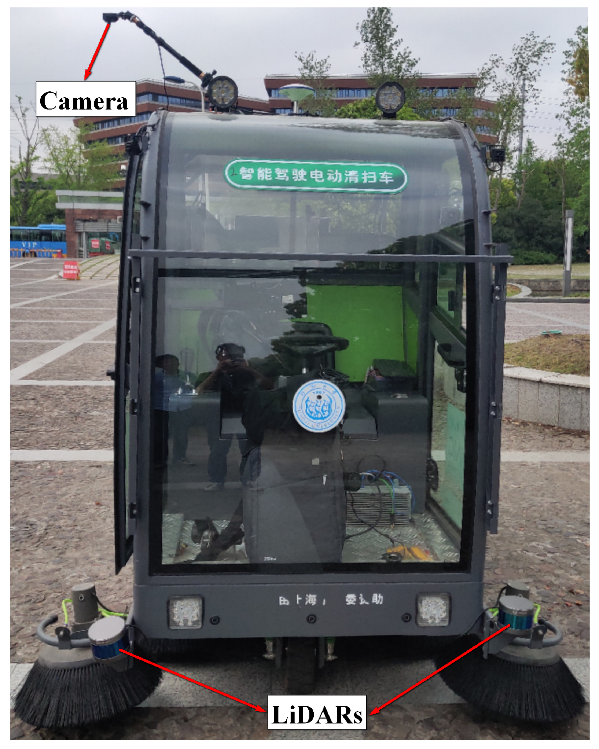
Our experiment vehicle is an intelligent sweeper developed at Tongji University (see Figure 4). The computing platform of this vehicle is a Nvidia Jetson TX2. A LiDAR-based lateral localization system is used by this vehicle, which is described in detail in Section 5.3.2. Two 16-layer LiDARs are equipped and mounted at the bottom of both sides of the vehicle (on top of the side brushes, see Figure 4). Our fish-eye camera is mounted on the right roof of the vehicle, which is the only sensor used by our proposed mono-vision based lateral localization system.
5.3.2. LiDAR-Based Lateral Localization System
The LiDAR-based lateral localization system is designed to keep a fixed close distance between the side brush of the sweeper and the curb. The distance is obtained via a LiDAR-based curb detection algorithm. The algorithm first selects candidates in the region of interest from the 3D point cloud generated by LiDARs. The region of interest here is within 1.5 m to the right and 2.5 m to the front of the center of the front axle of the vehicle. The heights of the selected candidates are in the range of 0.09 m to 0.11 m. After that, the algorithm selects the points closest to the vehicle on each row and fits them to a straight line using least squares. Then, the distance between the fitted straight line and the point 1.5 m ahead of the center of the front axle of the vehicle is calculated. The final output of the algorithm is the aforementioned distance minus one offset. An important assumption in this algorithm is that the height of curb is within a certain range, which is also widely used in other LiDAR-based curb detection methods. Consequently, the performance of the LiDAR-based lateral localization system could be greatly affected when the aforementioned assumption is not applicable.
5.3.3. Experimental Results
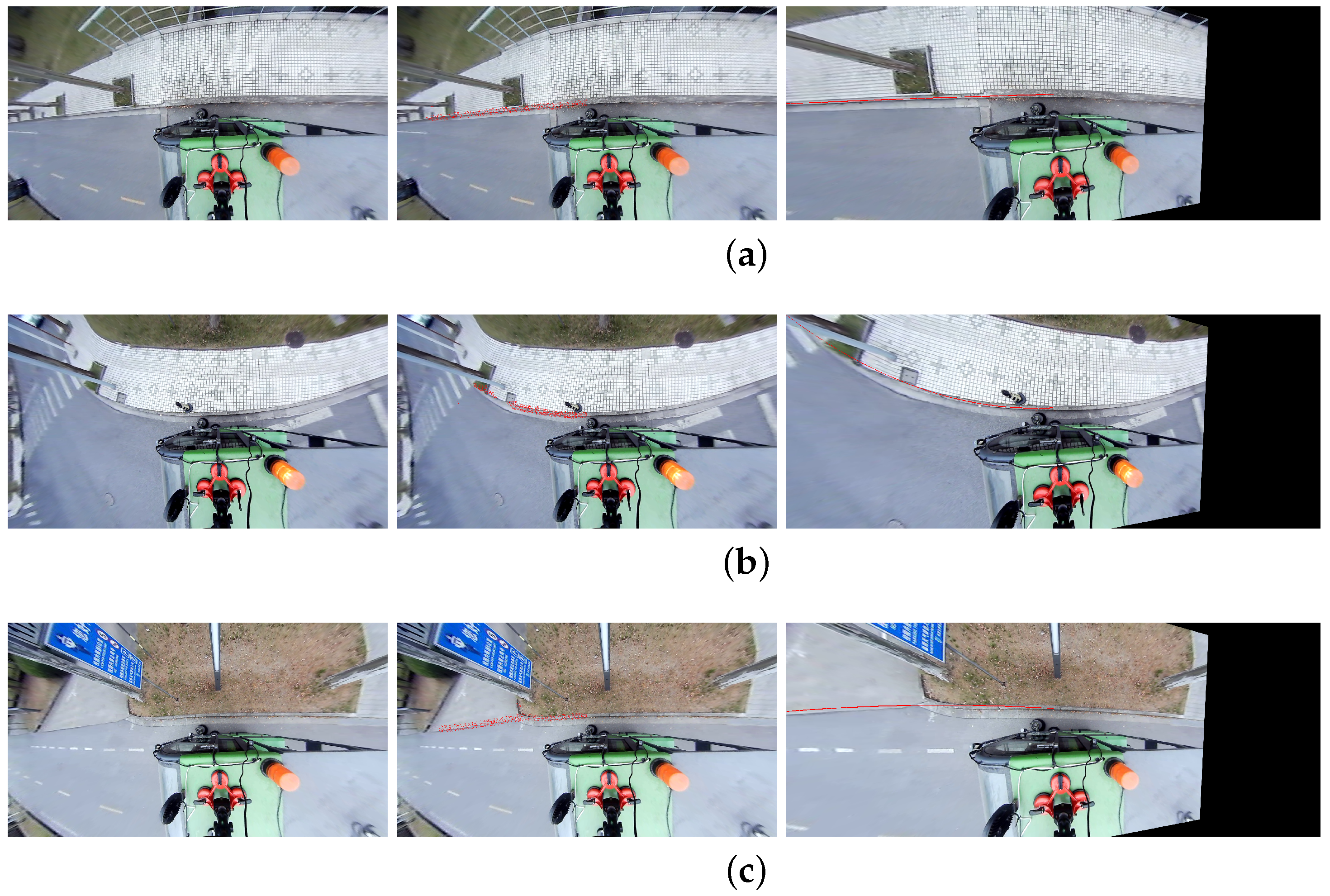
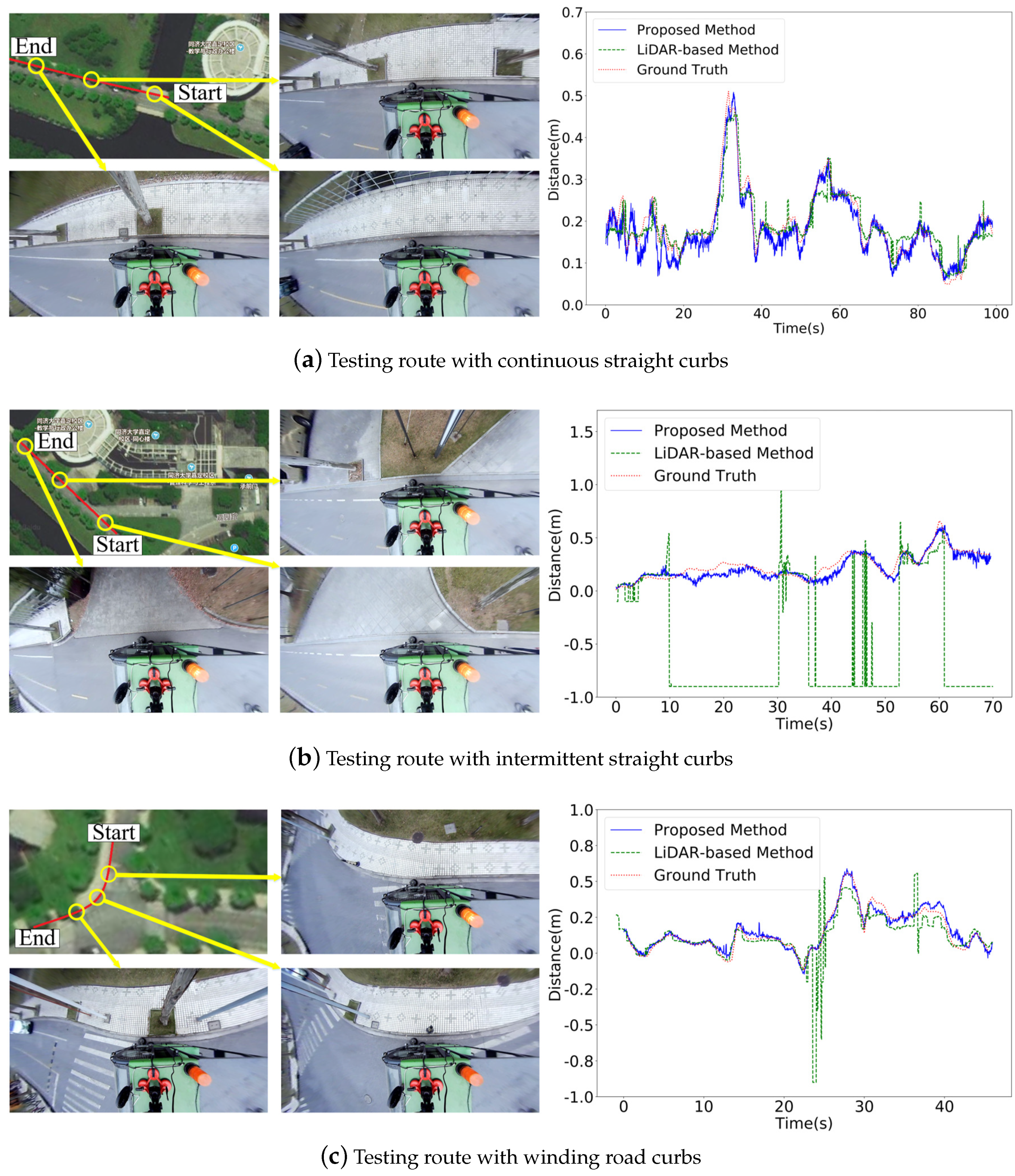
We select three representative testing routes (route with continuous straight curbs, route with intermittent straight curbs, route with curving curbs) for the autonomous sweeper. Figure 5 and Figure 6 show example scenes of these three routes. The curb detection results are shown in Figure 5. Based on the curb detection results of each frame (image frame for camera and point cloud frame for LiDAR), the lateral distance between the curbs and the sweepers is calculated. Experiments results with our proposed method, LiDAR-based method, and the ground truth are shown in Figure 6.
We evaluate the experiment results with two parameters: Average Error and Invalid Rate. The Average Error is defined as the average deviation of the calculated lateral distance value and the manually labeled ground truth. The Invalid Rate is the ratio of the number of failed curb detection frames to the number of all data frames in a testing route. If the deviation of the lateral distance calculated based on the curb detection result and the ground truth exceeds 0.1 m, the curb detection of the current frame is failed. The threshold 0.1 m is decided according the lateral localization accuracy of the intelligent sweeper. We show the experiment results in Table 2, Table 3 and Table 4.
(1) Testing route with continuous straight curbs
Table 2 shows that both the LiDAR-based method and the proposed method achieve high accuracy in terms of the Average Error. The Average Error is 0.022 m and 0.020 m for the LiDAR-based method and proposed method, respectively. In terms of the Invalid Rate, our proposed method performs better than the LiDAR-based method. The Invalid Rate is 0.7% and 0% for the LiDAR-based method and proposed method, respectively. It is likely that there are sudden height changes of the road curbs (e.g., at the timestamp of 40 s and 80 s in Figure 6a), which cause the failed curb detection of the LiDAR-based method while our proposed method is not affected.
(2) Testing route with intermittent straight curbs
In the testing route with intermittent straight curbs, the road curbs are intermittent. Typical scenes are from the intersections of the road and the trail, as shown in Figure 6b. As shown in Table 3, compared to the testing route with continuous straight curbs, the Average Error for LiDAR-based method and proposed method increases, and reaches 0.035 m and 0.038 m, respectively. In terms of the Invalid Rate, our proposed method achieves better performance than the LiDAR-based method. The main reason is that the LiDAR-based method assumes a certain height of the road curbs, while this assumption is not applied to the scenes such as road curbs at the intersections. The Invalid Rate for LiDAR-based method is up to 72.5%, which means that the results completely deviate (e.g., in the time interval of [10 s, 30 s] in Figure 6b). In comparison, the Invalid Rate of our proposed method is controlled at 9.2%.
(3) Testing route with winding road curbs
In testing route with winding road curbs, the road curbs are curved. Typical scenes are from the corners of the road, which are shown in Figure 6c. In Table 4, our proposed method achieves better performance in Average Error and Invalid Rate than the LiDAR-based method. The Average Error for the LiDAR-based method and proposed method is 0.032 m and 0.023 m, respectively. The Invalid Rate for our proposed method is 0.9%, which is much better than 12.1% for the LiDAR-based method. The reason for this phenomenon is that the LiDAR-based method has poor fitting performance on the curve (e.g., in the time interval of (22 s, 26 s) in Figure 6c).
6. Conclusions
We propose a mono-vision based lateral localization system of low-cost autonomous vehicles. Our system relies on a side-facing monocular fish-eye camera that precisely detects the road curbs with the proposed deep curb detection network. Compared with existing methods such as the global navigation satellite system and the LiDAR-based method, a monocular fish-eye camera is cheap, and our solution meets the low-price requirement of a low-speed low-cost autonomous vehicle such as sweepers. We conduct two experiments to evaluate the accuracy and robustness of our mono-vision based lateral localization. Our deep curb detection network achieves 93% pixel-level precision. Our experiment with the intelligent sweeper developed at Tongji University demonstrates that the average lateral distance error of our method is controlled within 0.035 m, and the maximum invalid rate is controlled within 9.2%.
In future work, several directions are worth investigating. Vision-based detection methods generally have problems that are easily affected by environmental factors such as the lighting. Thus, the combination of low-cost LiDAR (e.g., single layer laser scanner) and monocular camera could be a better solution. The future work will focus on how to efficiently fuse the data from the LiDAR and camera to develop a highly efficient and robust lateral localization system.
Author Contributions
J.Y. designs the method and performs the experiments; Z.Y. supervises the manuscripts. All authors have read and agreed to the published version of the manuscript.
Funding
The research leading to these results has partially received funding from the Shanghai Automotive Industry Sci-Tech Development Program according to Grant Agreement No. 1838, from the Shanghai AI Innovative Development Project, and from the State Key Laboratory of Advanced Design and Manufacturing for Vehicle Body according to Grant Agreement No.31815005.
Conflicts of Interest
The authors declare no conflict of interest.
References
- Zhou, J.; Yang, Y.; Zhang, J.; Edwan, E.; Loffeld, O.; Knedlik, S. Tightly-coupled INS/GPS using Quaternion-based Unscented Kalman filter. In Proceedings of the AIAA Guidance, Navigation, and Control Conference, Portland, Oregon, 8–11 August 2011; p. 6488. [Google Scholar]
- Enkhtur, M.; Cho, S.Y.; Kim, K.H. Modified unscented Kalman filter for a multirate INS/GPS integrated navigation system. Etri J. 2013, 35, 943–946. [Google Scholar] [CrossRef] [Green Version]
- Suhr, J.K.; Jang, J.; Min, D.; Jung, H.G. Sensor fusion-based low-cost vehicle localization system for complex urban environments. IEEE Trans. Intell. Transp. Syst. 2017, 18, 1078–1086. [Google Scholar] [CrossRef]
- Vu, A.; Ramanandan, A.; Chen, A.; Farrell, J.A.; Barth, M. Real-time computer vision/DGPS-aided inertial navigation system for lane-level vehicle navigation. IEEE Trans. Intell. Transp. Syst. 2012, 13, 899–913. [Google Scholar] [CrossRef]
- Sefati, M.; Daum, M.; Sondermann, B.; Kreisköther, K.D.; Kampker, A. Improving vehicle localization using semantic and pole-like landmarks. In Proceedings of the 2017 IEEE Intelligent Vehicles Symposium (IV), Los Angeles, CA, USA, 11–14 June 2017; pp. 13–19. [Google Scholar]
- Im, J.H.; Im, S.H.; Jee, G.I. Vertical corner feature based precise vehicle localization using 3D LIDAR in urban area. Sensors 2016, 16, 1268. [Google Scholar] [CrossRef] [PubMed] [Green Version]
- Tao, Z.; Bonnifait, P.; Fremont, V.; Ibanez-Guzman, J. Mapping and localization using GPS, lane markings and proprioceptive sensors. In Proceedings of the 2013 IEEE/RSJ International Conference on Intelligent Robots and Systems, Tokyo, Japan, 3–7 November 2013; pp. 406–412. [Google Scholar]
- Gruyer, D.; Belaroussi, R.; Revilloud, M. Accurate lateral positioning from map data and road marking detection. Expert Syst. Appl. 2016, 43, 1–8. [Google Scholar] [CrossRef]
- Seo, Y.W.; Rajkumar, R. Tracking and estimation of ego-vehicle’s state for lateral localization. In Proceedings of the 17th International IEEE Conference on Intelligent Transportation Systems (ITSC), Qingdao, China, 8–11 October 2014; pp. 1251–1257. [Google Scholar]
- Wang, L.; Zhang, Y.; Wang, J. Map-based localization method for autonomous vehicles using 3D-LIDAR. IFAC-PapersOnLine 2017, 50, 276–281. [Google Scholar] [CrossRef]
- Meng, X.; Wang, H.; Liu, B. A robust vehicle localization approach based on gnss/imu/dmi/lidar sensor fusion for autonomous vehicles. Sensors 2017, 17, 2140. [Google Scholar] [CrossRef] [PubMed]
- Zhao, G.; Yuan, J. Curb detection and tracking using 3D-LIDAR scanner. In Proceedings of the 2012 19th IEEE International Conference on Image Processing, Orlando, FL, USA, 30 September–3 October 2012; pp. 437–440. [Google Scholar]
- Zhang, Y.; Wang, J.; Wang, X.; Dolan, J.M. Road-segmentation-based curb detection method for self-driving via a 3D-LiDAR sensor. IEEE Trans. Intell. Transp. Syst. 2018, 19, 3981–3991. [Google Scholar] [CrossRef]
- Fernández, C.; Llorca, D.F.; Stiller, C.; Sotelo, M. Curvature-based curb detection method in urban environments using stereo and laser. In Proceedings of the 2015 IEEE Intelligent Vehicles Symposium (IV), Seoul, Korea, 28 June–1 July 2015; pp. 579–584. [Google Scholar]
- Cheng, M.; Zhang, Y.; Su, Y.; Alvarez, J.M.; Kong, H. Curb detection for road and sidewalk detection. IEEE Trans. Veh. Technol. 2018, 67, 10330–10342. [Google Scholar] [CrossRef]
- Kellner, M.; Hofmann, U.; Bouzouraa, M.E.; Stephan, N. Multi-cue, model-based detection and mapping of road curb features using stereo vision. In Proceedings of the 2015 IEEE 18th International Conference on Intelligent Transportation Systems, Gran Canaria, Spain, 15–18 September 2015; pp. 1221–1228. [Google Scholar]
- Ronneberger, O.; Fischer, P.; Brox, T. U-net: Convolutional networks for biomedical image segmentation. In International Conference on Medical Image Computing and Computer-Assisted Intervention; Springer: Berlin, Germany, 2015; pp. 234–241. [Google Scholar]
- Pan, X.; Shi, J.; Luo, P.; Wang, X.; Tang, X. Spatial as deep: Spatial cnn for traffic scene understanding. In Proceedings of the Thirty-Second AAAI Conference on Artificial Intelligence, New Orleans, LA, USA, 15–18 February 2018. [Google Scholar]
- Suleymanov, T.; Amayo, P.; Newman, P. Inferring road boundaries through and despite traffic. In Proceedings of the 2018 21st International Conference on Intelligent Transportation Systems (ITSC), Maui, HI, USA, 4–7 November 2018; pp. 409–416. [Google Scholar]
- Siegemund, J.; Pfeiffer, D.; Franke, U.; Förstner, W. Curb reconstruction using conditional random fields. In Proceedings of the 2010 IEEE Intelligent Vehicles Symposium, La Jolla, CA, USA, 21–24 June 2010; pp. 203–210. [Google Scholar]
- Rhee, J.H.; Seo, J. Low-Cost Curb Detection and Localization System Using Multiple Ultra sonic Sensors. Sensors 2019, 19, 1389. [Google Scholar] [CrossRef] [PubMed] [Green Version]
- Simonyan, K.; Zisserman, A. Very deep convolutional networks for large-scale image recognition. arXiv 2014, arXiv:1409.1556. [Google Scholar]
- Girshick, R.; Donahue, J.; Darrell, T.; Malik, J. Rich feature hierarchies for accurate object detection and semantic segmentation. In Proceedings of the IEEE conference on computer vision and pattern recognition, Columbus, OH, USA, 23–28 June 2014; pp. 580–587. [Google Scholar]
- Girshick, R. Fast r-cnn. In Proceedings of the IEEE International Conference on Computer Vision, Santiago, Chile, 7–13 December 2015; pp. 1440–1448. [Google Scholar]
- Ren, S.; He, K.; Girshick, R.; Sun, J. Faster r-cnn: Towards real-time object detection with region proposal networks. Advances in neural information processing systems. arXiv 2015, arXiv:1506.01497. [Google Scholar]
- Paszke, A.; Gross, S.; Chintala, S.; Chanan, G.; Yang, E.; DeVito, Z.; Lin, Z.; Desmaison, A.; Antiga, L.; Lerer, A. Automatic Differentiation in PyTorch. Long Beach, CA, USA. 2017. Available online: https://openreview.net/forum?id=BJJsrmfCZ (accessed on 11 March 2021).
Figure 1.
Hierarchical structure of the proposed mono-vision based lateral localization system. The upper layer (the first row) is the lateral localization system. Depending on the curb detection results, the vehicle calculates the lateral distance between itself and the nearest road curb which is then sent to the vehicle control system. The middle layer (the second row) is the core component of our system, which is a deep curb detection network. It consists of three important modules: road scene classification module, curb region of interest module, and semantic segmentation module. The bottom layer (the third row) shows the network architecture of our semantic segmentation module, which is built based on U-Net [17] and SCNN [18].

Figure 2.
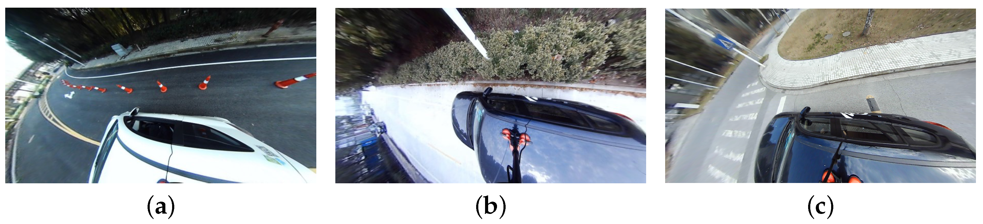
Road scene samples of three classes: (a) road scene with obstacles; (b) road scene with curbs; (c) road scene with intersection.
Figure 2.
Road scene samples of three classes: (a) road scene with obstacles; (b) road scene with curbs; (c) road scene with intersection.

Figure 3.
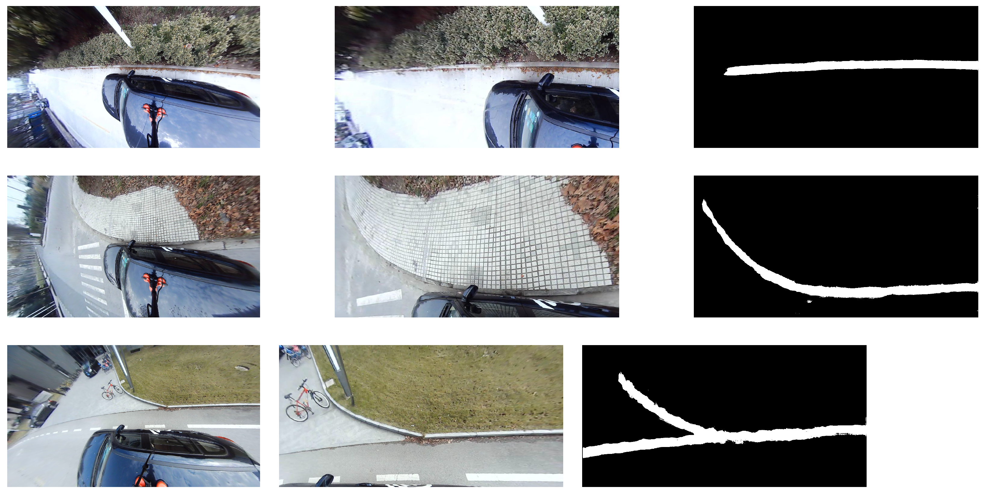
Detection results of deep curb detection network. Left column: image samples from the dataset; Middle Column: enlarged curb regions of interests extracted by CRoI module; Right column: curb segmentation results.
Figure 3.
Detection results of deep curb detection network. Left column: image samples from the dataset; Middle Column: enlarged curb regions of interests extracted by CRoI module; Right column: curb segmentation results.

Figure 4.
The intelligent sweeper of Tongji University.

Figure 5.
Experimental results of the deep curb detection network with autonomous sweeper. (a) curb detection results of the testing route with continuous straight curbs. Left image is a sample. Middle image shows the curb detection results which are highlighted by red color. Right image shows a fitted curve based on the curb detection results. Right image is converted into bird-view; (b) curb detection results of the testing route with intermittent straight curbs; (c) curb detection results of the testing route with winding road curbs.

Figure 6.
Experimental results with autonomous sweeper. (a) testing route with continuous straight curb. The left figure shows the satellite images and sampled scenes. The right figure shows the lateral localization results of the proposed method, LiDAR-based method and ground truth; (b) testing route with intermittent straight curbs; (c) testing route with winding road curbs.


Table 1.
Experiment results of semantic segmentation.
| Models | Computing Time (ms) | |
|---|---|---|
| Our algorithm | 93.86 | 92 |
| Full U-Net | 90.34 | 91 |
Table 2.
Average error and invalid rate of the testing route with continuous straight curbs.
| Evaluation Metrics | Proposed Method | LiDAR-Based Method |
|---|---|---|
| Average Error (m) | 0.020 | 0.022 |
| Invalid Rate | 0% | 0.7% |
Table 3.
Average error and invalid rate of the testing route with intermittent straight curbs.
| Evaluation Metrics | Proposed Method | LiDAR-Based Method |
|---|---|---|
| Average Error (m) | 0.035 | 0.038 |
| Invalid Rate | 9.2% | 72.5% |
Table 4.
Average error and invalid rate of the testing route with curving curbs.
| Evaluation Metrics | Proposed Method | LiDAR-Based Method |
|---|---|---|
| Average Error (m) | 0.023 | 0.032 |
| Invalid Rate | 0.9% | 12.1% |
Publisher’s Note: MDPI stays neutral with regard to jurisdictional claims in published maps and institutional affiliations. |
© 2021 by the authors. Licensee MDPI, Basel, Switzerland. This article is an open access article distributed under the terms and conditions of the Creative Commons Attribution (CC BY) license (http://creativecommons.org/licenses/by/4.0/).
Share and Cite
MDPI and ACS Style
Yu, J.; Yu, Z. Mono-Vision Based Lateral Localization System of Low-Cost Autonomous Vehicles Using Deep Learning Curb Detection. Actuators 2021, 10, 57. https://0-doi-org.brum.beds.ac.uk/10.3390/act10030057
AMA Style
Yu J, Yu Z. Mono-Vision Based Lateral Localization System of Low-Cost Autonomous Vehicles Using Deep Learning Curb Detection. Actuators. 2021; 10(3):57. https://0-doi-org.brum.beds.ac.uk/10.3390/act10030057
Chicago/Turabian StyleYu, Junwei, and Zhuoping Yu. 2021. "Mono-Vision Based Lateral Localization System of Low-Cost Autonomous Vehicles Using Deep Learning Curb Detection" Actuators 10, no. 3: 57. https://0-doi-org.brum.beds.ac.uk/10.3390/act10030057
Note that from the first issue of 2016, this journal uses article numbers instead of page numbers. See further details here.