
Sensorless Pedalling Torque Estimation Based on Motor Load Torque Observation for Electrically Assisted Bicycles


Abstract
:1. Introduction
2. Theory
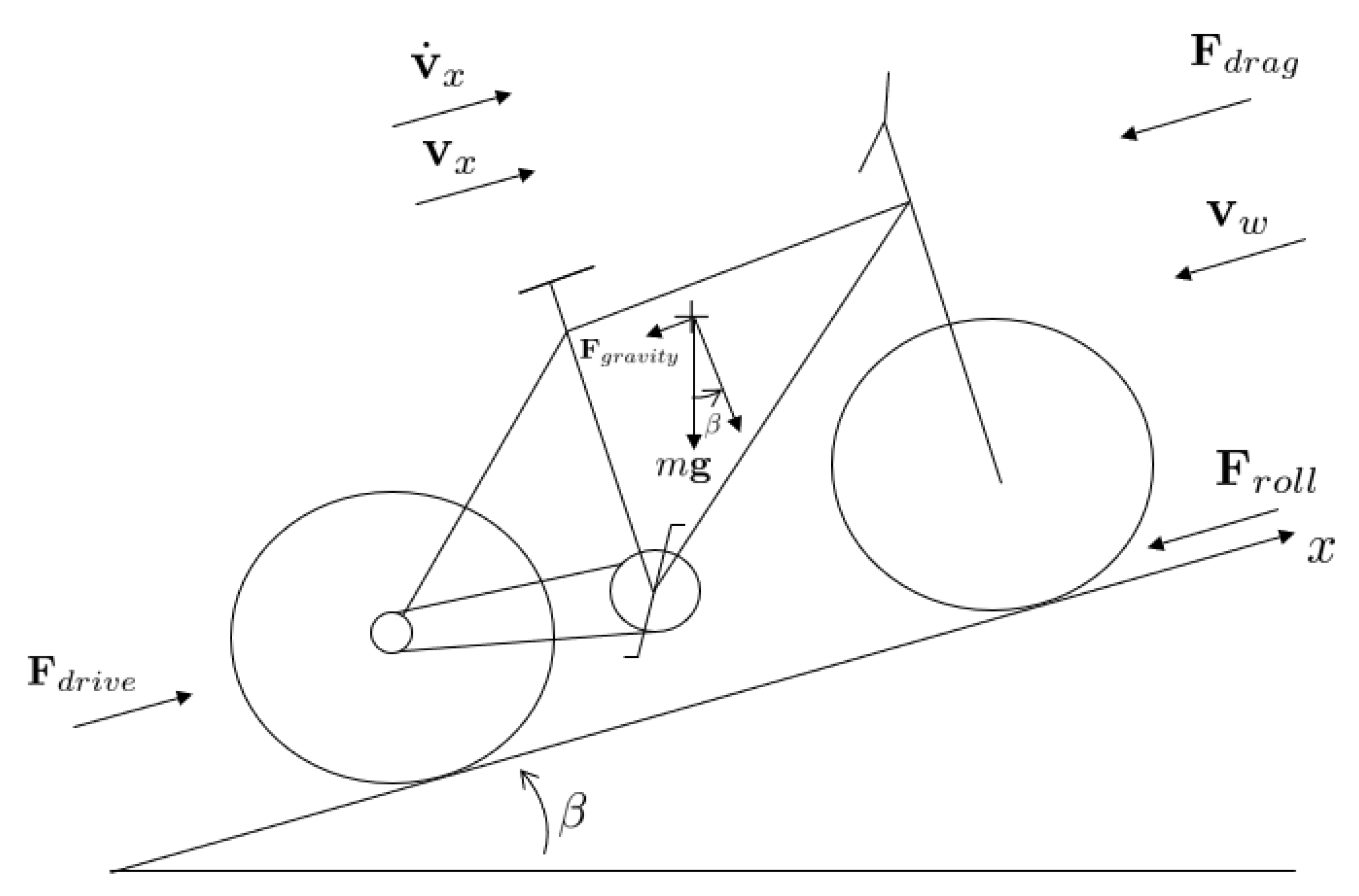
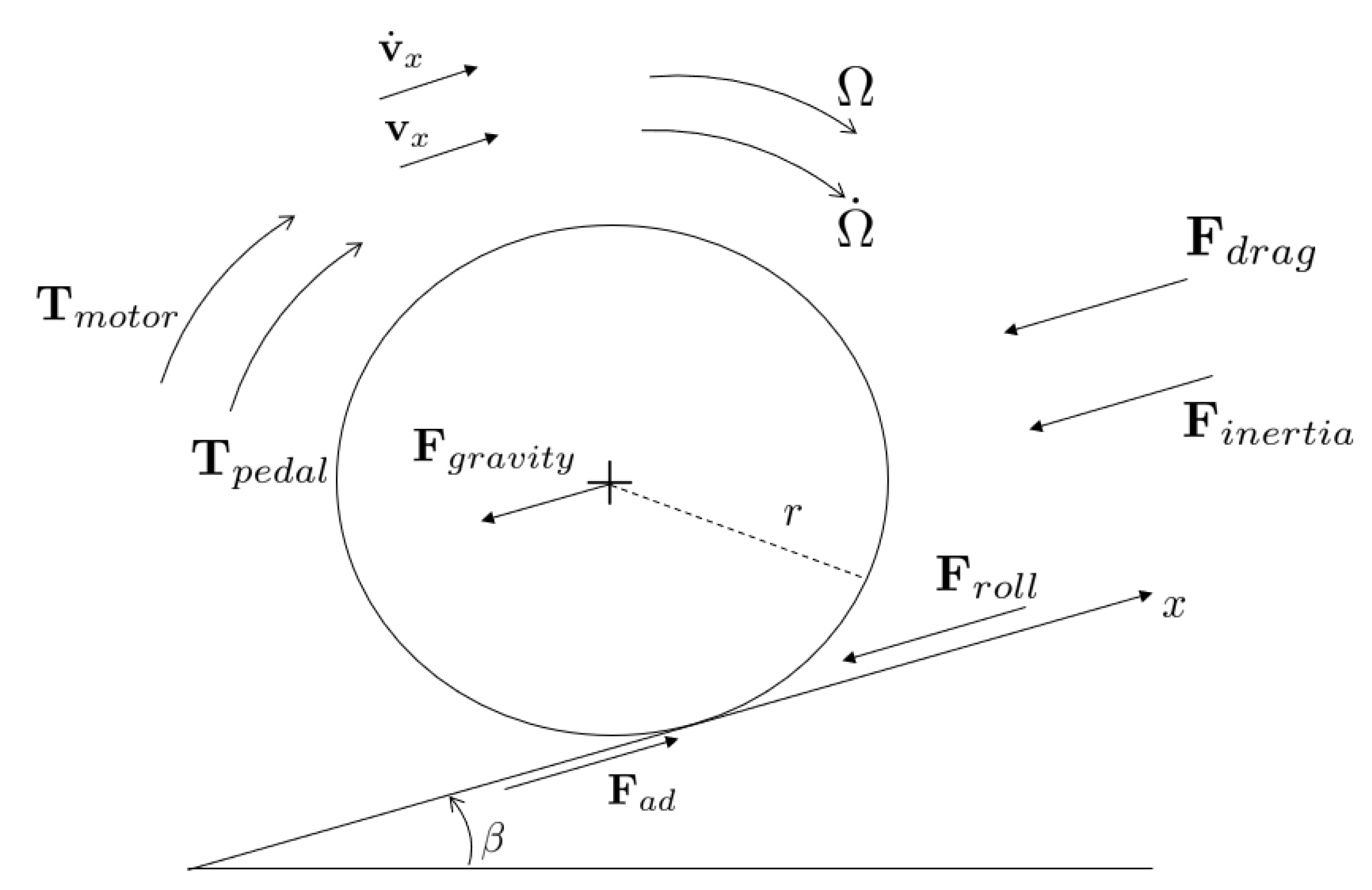
2.1. Bicycle Longitudinal Dynamics
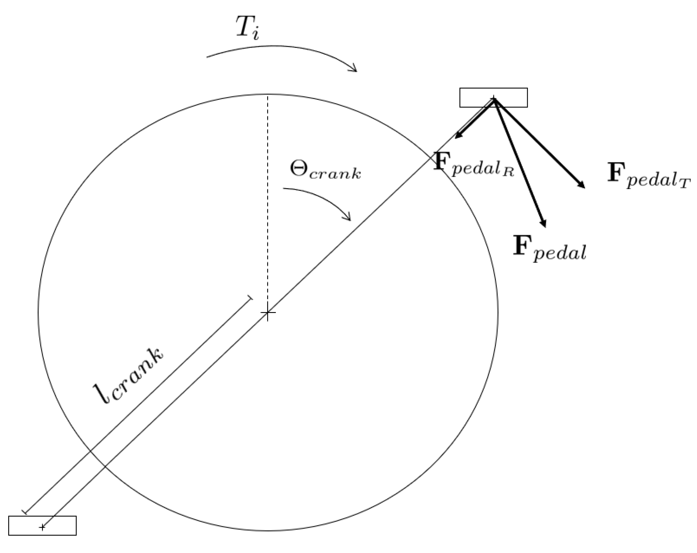
2.2. Pedalling Torque Estimation
2.3. Motor Load Torque Observation
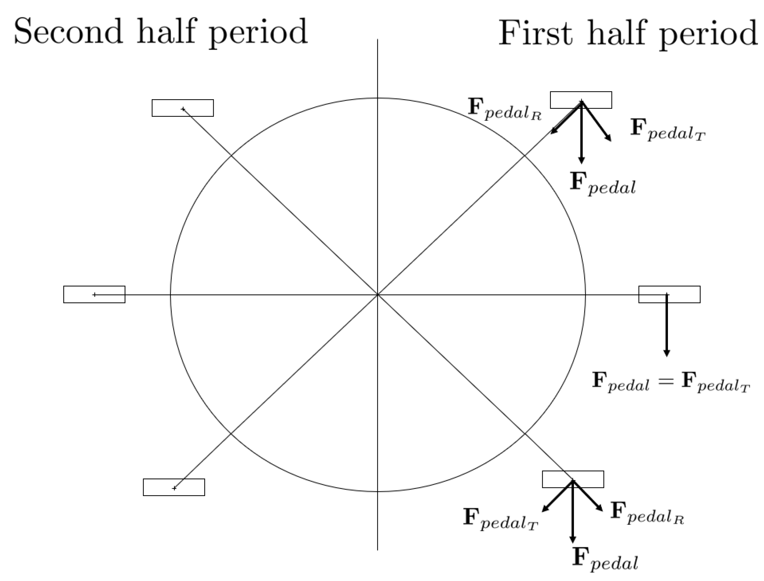
2.4. Pedalling Torque Analysis
3. Experimental Validation
3.1. Experimental Setup Description
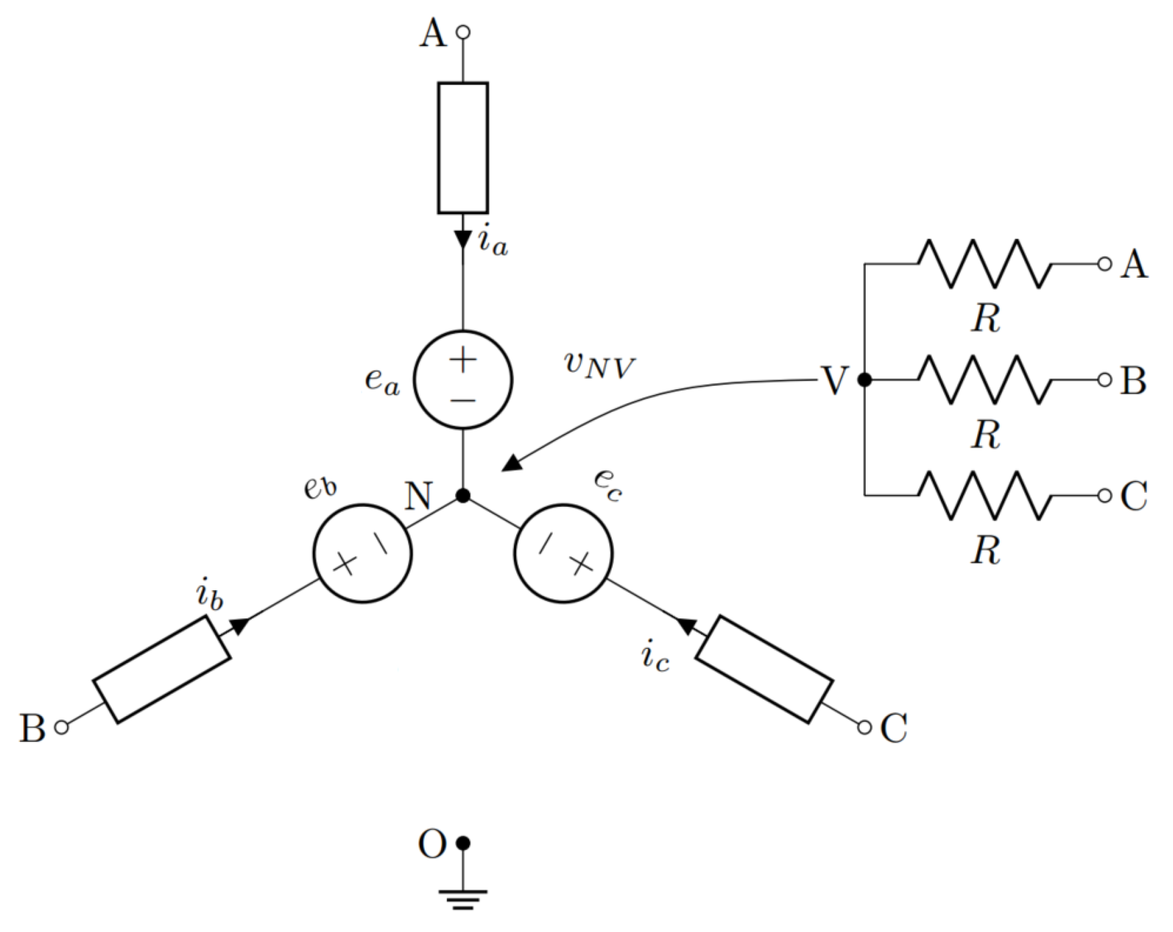
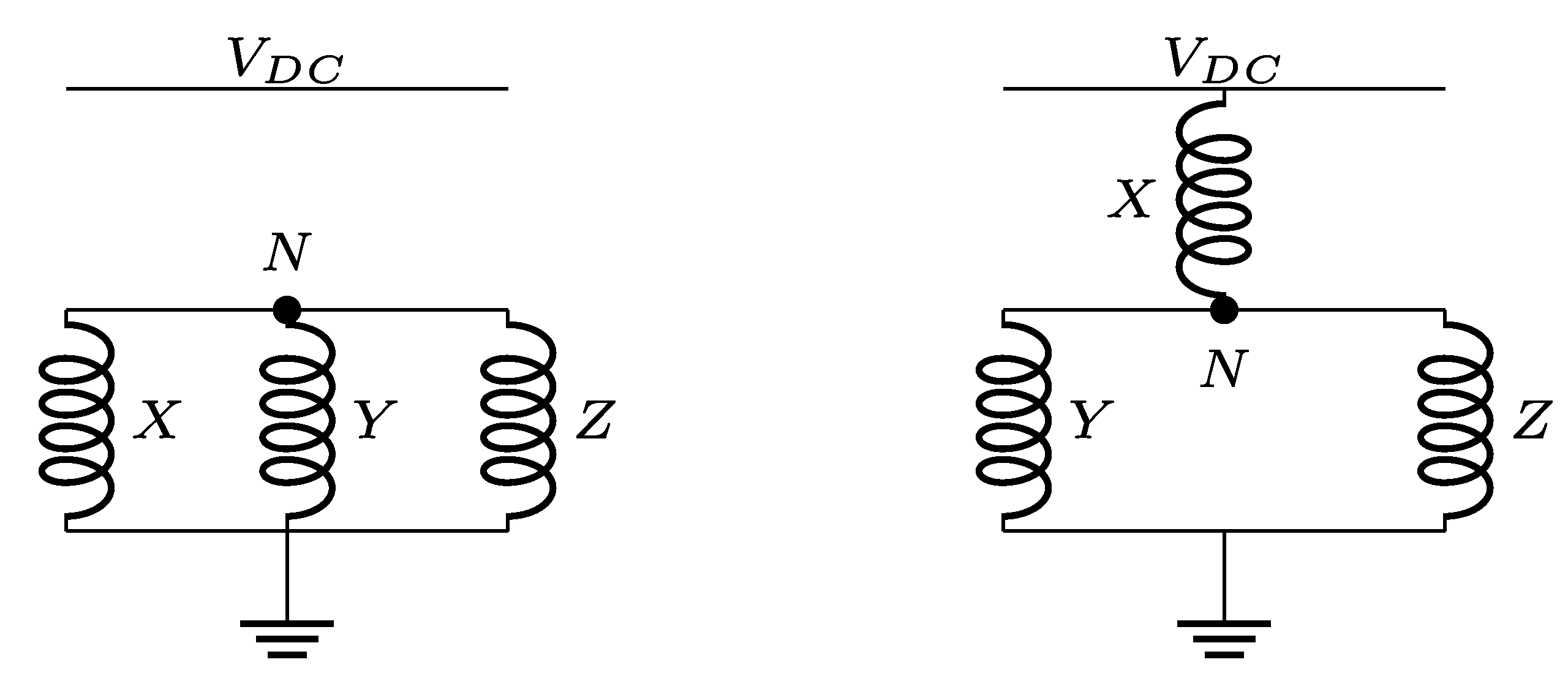
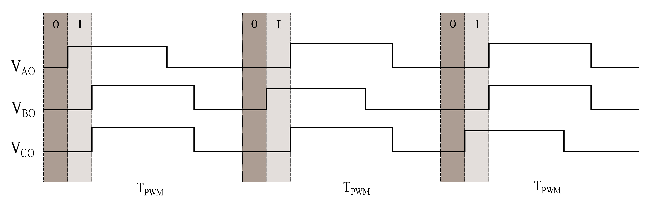
3.2. Direct Flux Control DFC Sensorless Technique
3.3. Electrical Parameters Identification
3.4. Control System Design
3.5. Mechanical Parameters Identification
4. Pedalling Torque Estimation
4.1. Pedalling Torque Observer
4.2. Pedalling Torque Reconstruction
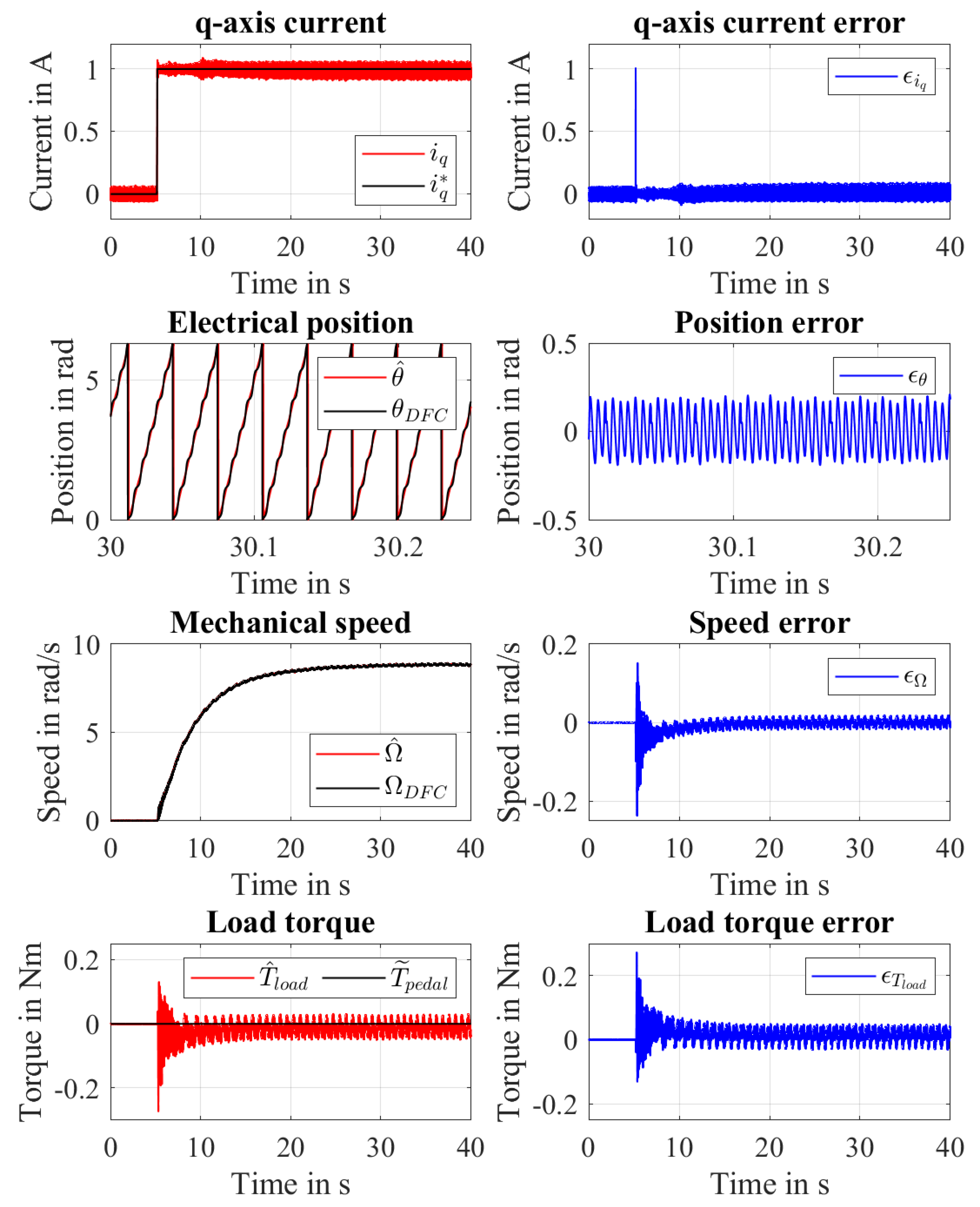
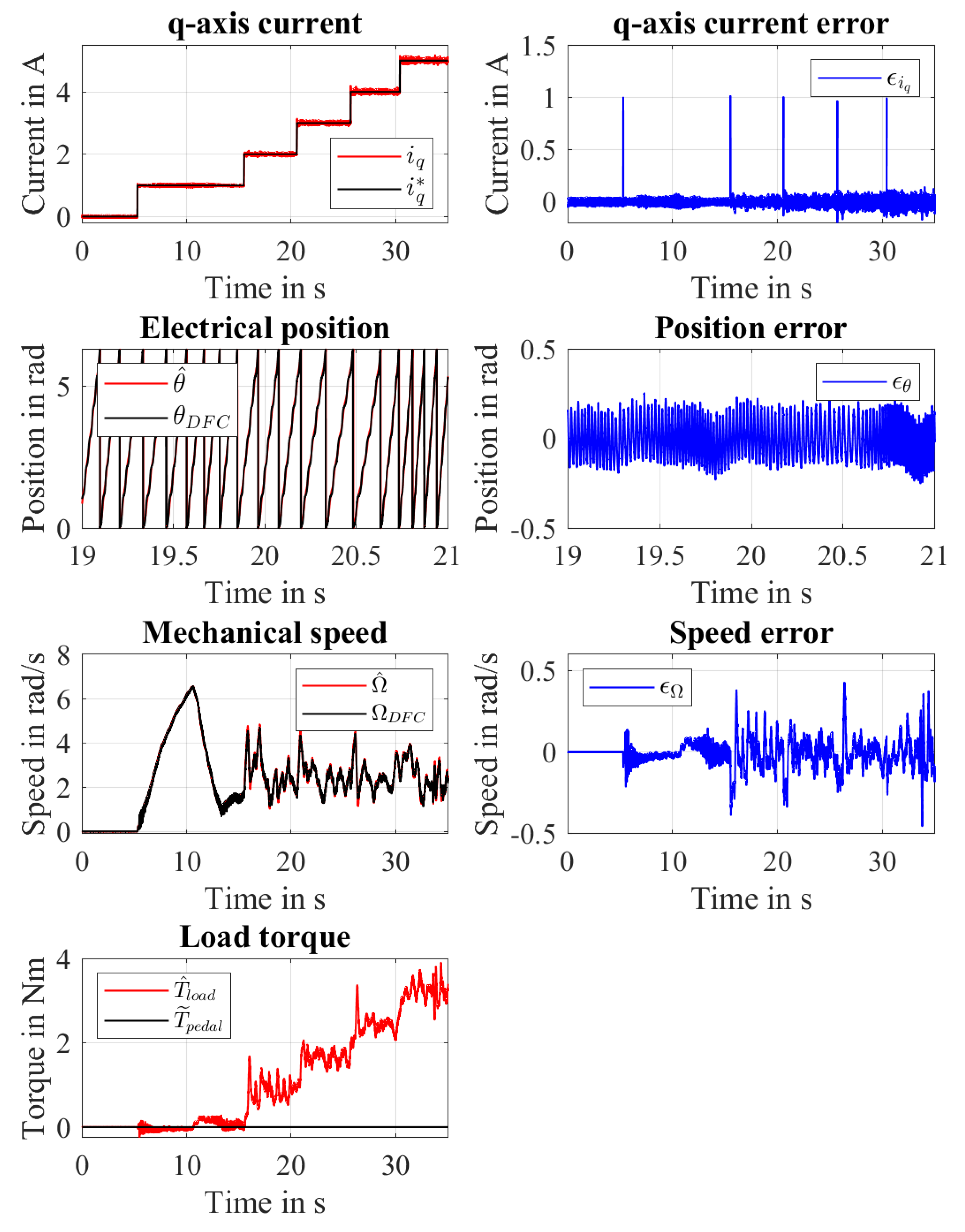
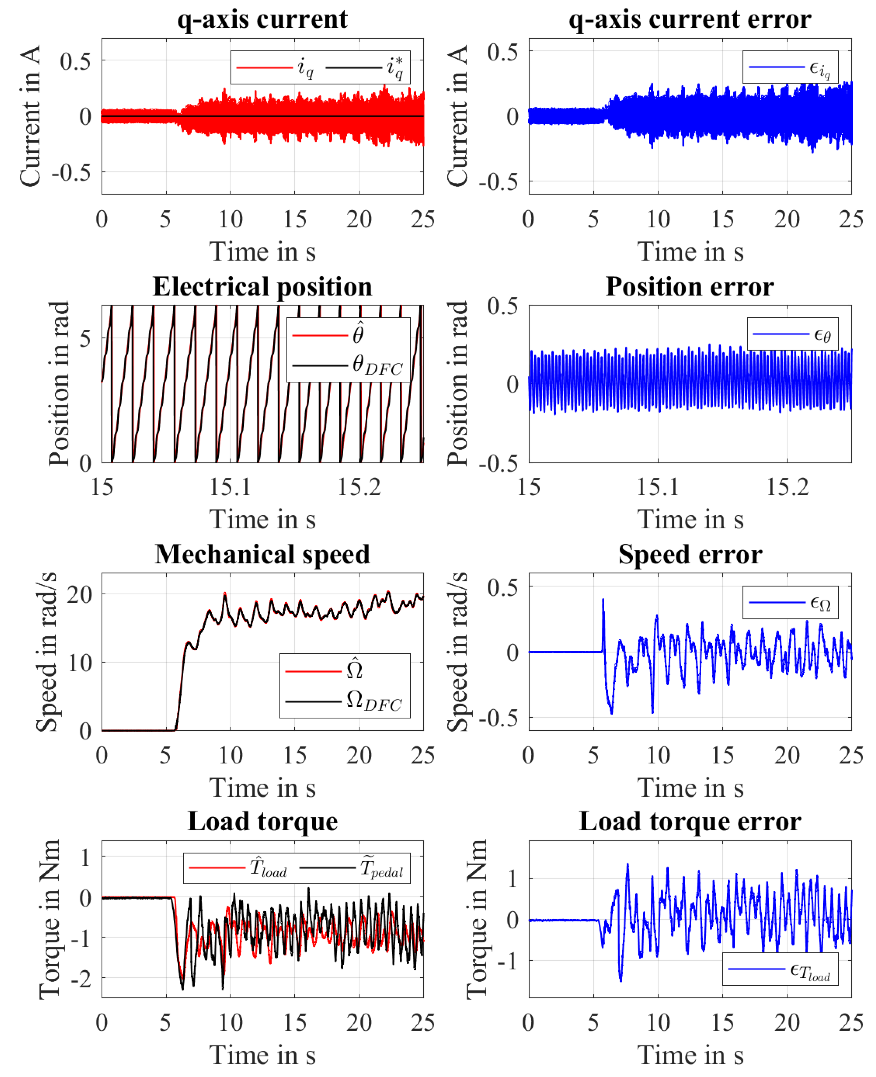
4.3. Load Torque Observer LTO Validation
- E1:
- the motor is current controlled with A and A without an applied load torque Nm;
- E2:
- the motor is current controlled with progressively increasing steps and A and an external torque disturbance is applied ;
- E3:
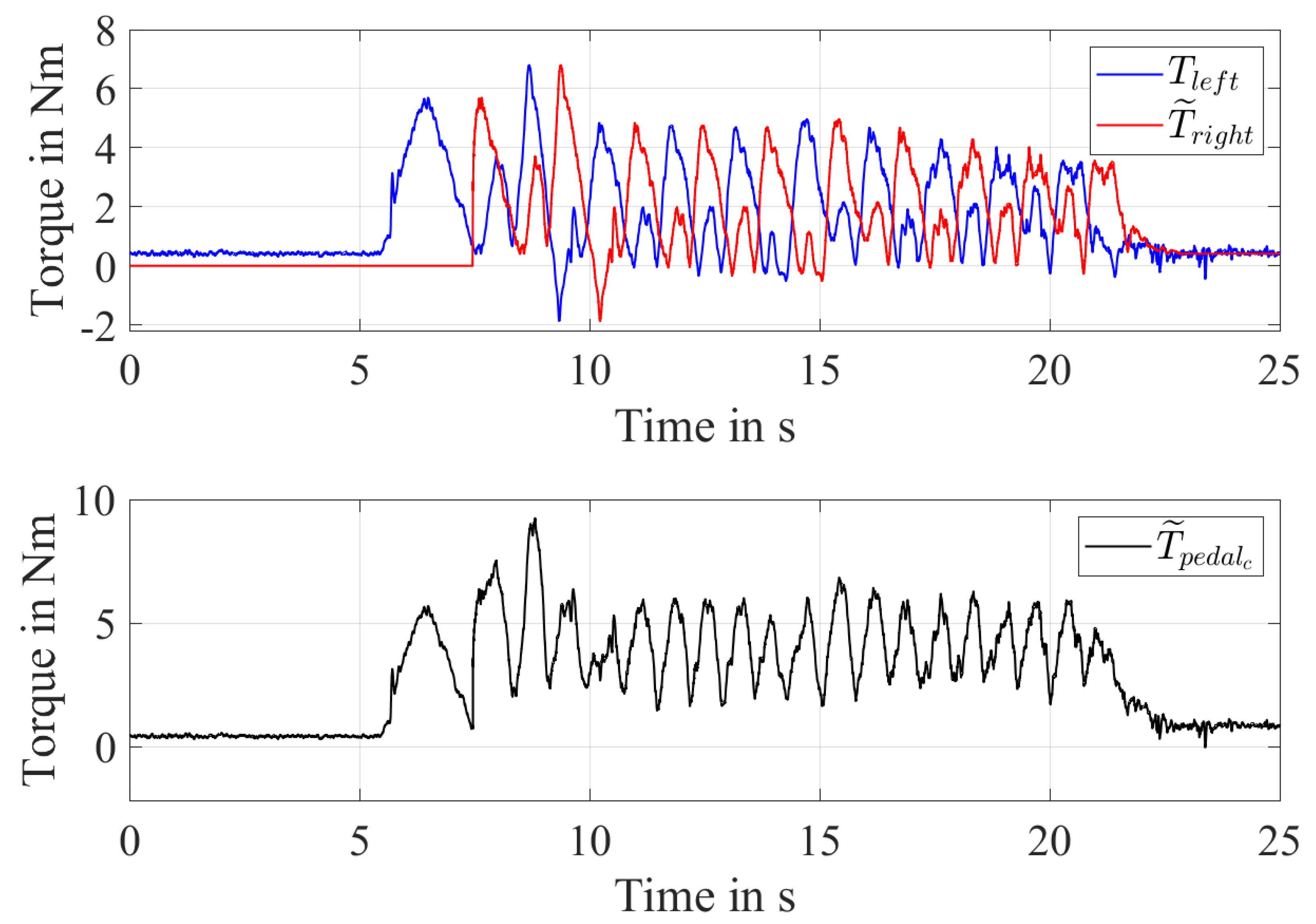
- the motor is current controlled with A and A and a pedalling torque is applied .
- E4:
- the motor is current controlled with A and A and both a pedalling torque and an external torque disturbance are applied .
- the provided current reference given by the motor current control with the actual current ;
- the measured electrical rotor position obtained applying the DFC technique with the estimated electrical rotor position given by the LTO ;
- the measured rotor speed obtained as the derivative of the DFC rotor position with the estimated rotor speed given by the LTO ;
- the reconstructed pedalling torque reported to the motor side with the estimated motor load torque given by the LTO .
5. Conclusions
Author Contributions
Funding
Institutional Review Board Statement
Informed Consent Statement
Data Availability Statement
Acknowledgments
Conflicts of Interest
References
- Muetze, A.; Tan, Y.C. Electric bicycles—A performance evaluation. IEEE Ind. Appl. Mag. 2007, 13, 12–21. [Google Scholar] [CrossRef]
- Cappelle, J.; Lataire, P.; Maggetto, G.; Van den Bossche, P.; Timmermans, J. Electrically Assisted Cycling around the World. In Proceedings of the 20th International Electric Vehicle Symposium (EVS 20), Long Beach, CA, USA, 15–19 November 2003. [Google Scholar]
- Ohnishi, K. A new servo method in mechatronics. Trans. Jpn. Soc. Electr. Eng. 1987, 107-D, 83–86. [Google Scholar]
- Murakami, T.; Ohnishi, K. Advanced motion control in mechatronics—A tutorial. In Proceedings of the IEEE International Workshop on Intelligent Control, Istanbul, Turkey, 20–22 August 1990; Volume 1, pp. SL9–SL17. [Google Scholar]
- Cheon, D.S.; Nam, K.H. Pedaling torque sensor-less power assist control of an electric bike via model-based impedance control. Int. J. Automot. Technol. 2017, 18, 327–333. [Google Scholar] [CrossRef]
- Sankaranarayanan, V.; Ravichandran, S. Torque sensorless control of a human-electric hybrid bicycle. In Proceedings of the International Conference on Industrial Instrumentation and Control (ICIC), Pune, India, 28–30 May 2015; pp. 806–810. [Google Scholar]
- Oh, S.; Ohri, Y. Sensor Free Power Assisting Control Based on Velocity Control and Disturbance Observer. In Proceedings of the IEEE International Symposium on Industrial Electronics (ISIE 2005), Dubrovnik, Croatia, 20–23 June 2005; pp. 1709–1714. [Google Scholar]
- Ohnishi, K.; Matsui, N.; Hori, Y. Estimation, identification, and sensorless control in motion control system. Proc. IEEE 1994, 82, 1253–1265. [Google Scholar] [CrossRef]
- Seki, H.; Iso, M.; Hori, Y. How to design force sensorless power assist robot considering environmental characteristics-position control based or force control based. In Proceedings of the IEEE 2002 28th Annual Conference of the Industrial Electronics Society (IECON 02), Seville, Spain, 5–8 November 2002; Volume 3, pp. 2255–2260. [Google Scholar]
- Kato, A.; Ohnishi, K. Robust force sensorless control in motion control system. In Proceedings of the 9th IEEE International Workshop on Advanced Motion Control, Istanbul, Turkey, 27–29 March 2006; pp. 165–170. [Google Scholar]
- Salvucci, V.; Oh, S.; Hori, Y. New approach to force sensor-less power assist control for high friction and high inertia systems. In Proceedings of the IEEE International Symposium on Industrial Electronics, Bari, Italy, 4–7 July 2010; pp. 3559–3564. [Google Scholar]
- Nam, K.; Kim, Y.; Oh, S.; Hori, Y. Steering Angle-Disturbance Observer (SA-DOB) based yaw stability control for electric vehicles with in-wheel motors. In Proceedings of the IICCAS 2010, Gyeonggi-do, Korea, 27–30 October 2010; pp. 1303–1307. [Google Scholar]
- Nam, K.; Fujimoto, H.; Hori, Y. Advanced Motion Control of Electric Vehicles Based on Robust Lateral Tire Force Control via Active Front Steering. IEEE/ASME Trans. Mechatron. 2014, 19, 289–299. [Google Scholar] [CrossRef]
- Kurosawa, T.; Fujimoto, Y.; Tokumaru, T. Estimation of pedaling torque for electric power assisted bicycles. In Proceedings of the IECON 2014—40th Annual Conference of the IEEE Industrial Electronics Society, Dallas, TX, USA, 29 October–1 November 2014; pp. 2756–2761. [Google Scholar]
- Kurosawa, T.; Fujimoto, Y. Torque Sensorless Control for an Electric Power Assisted Bicycle with Instantaneous Pedaling Torque Estimation. IEEJ J. Ind. Appl. 2017, 6, 124–129. [Google Scholar] [CrossRef]
- Fukushima, N.; Fujimoto, Y. Estimation of pedaling torque for electric power-assisted bicycle on slope environment. In Proceedings of the IEEE International Conference on Advanced Intelligent Mechatronics (AIM), Munich, Germany, 3–7 July 2017; pp. 1682–1687. [Google Scholar]
- Fukushima, N.; Fujimoto, Y. Experimental verification of torque sensorless control for electric power-assisted bicycles on sloped environment. In Proceedings of the IEEE 15th International Workshop on Advanced Motion Control (AMC), Tokyo, Japan, 9–11 March 2018; pp. 66–71. [Google Scholar]
- Fan, X.; Tomizuka, M. Robust disturbance observer design for a power-assist electric bicycle. In Proceedings of the 2010 American Control Conference, Baltimore, MD, USA, 30 June–2 July 2010; pp. 1166–1171. [Google Scholar]
- Chew, K.K.; Tomizuka, M. Digital control of repetitive errors in disk drive systems. IEEE Control. Syst. Mag. 1990, 10, 16–20. [Google Scholar] [CrossRef]
- Steinbuch, M. Repetitive control for systems with uncertain period-time. Automatica 2002, 38, 2103–2109. [Google Scholar] [CrossRef]
- Tsao, T.C.; Tomizuka, M. Robust Adaptive and Repetitive Digital Tracking Control and Application to a Hydraulic Servo for Noncircular Machining. J. Dyn. Syst. Meas. Control. 1994, 116, 24–32. [Google Scholar] [CrossRef]
- Hanson, R.D.; Tsao, T.C. Periodic Sampling Interval Repetitive Control and Its Application to Variable Spindle Speed Noncircular Turning Process. J. Dyn. Syst. Meas. Control. 1998, 122, 560–566. [Google Scholar] [CrossRef]
- Hatada, K.; Hirata, K. Energy-efficient power assist control for periodic motions. In Proceedings of the SICE Annual Conference 2010, Taipei, Taiwan, 18–21 August 2010; pp. 2004–2009. [Google Scholar]
- Hatano, R.; Namikawa, D.; Minagawa, R.; Iwase, M. Experimental verification of effectiveness on driving force assist control based on repetitive control for electrically-assisted bicycles. In Proceedings of the IEEE 13th International Workshop on Advanced Motion Control (AMC), Yokohama, Japan, 14–16 March 2014; pp. 237–241. [Google Scholar]
- Fan, X.; Iwase, M.; Tomizuka, M. Non-Uniform Velocity Profile Compensation for an Electric Bicycle Based on Repetitive Control With Sinusoidal and Non-Sinusoidal Internal Models. In Proceedings of the SME 2009 Dynamic Systems and Control Conference, Hollywood, CA, USA, 12–14 October 2009; Volume 1, pp. 765–772. [Google Scholar]
- Solsona, J.; Valla, M.I.; Muravchik, C. Nonlinear control of a permanent magnet synchronous motor with disturbance torque estimation. IEEE Trans. Energy Convers. 2000, 15, 163–168. [Google Scholar] [CrossRef]
- Aghili, F. Torque control of electric motors without using torque sensor. In Proceedings of the International Conference on Intelligent Robots and Systems, San Diego, CA, USA, 29 October–2 November 2007; pp. 3604–3609. [Google Scholar]
- Lian, C.; Xiao, F.; Gao, S.; Liu, J. Load Torque and Moment of Inertia Identification for Permanent Magnet Synchronous Motor Drives Based on Sliding Mode Observer. IEEE Trans. Power Electron. 2019, 34, 5675–5683. [Google Scholar] [CrossRef]
- Zedong, Z.; Yongdong, L.; Fadel, M.; Xi, X. A Rotor Speed and Load Torque Observer for PMSM Based on Extended Kalman Filter. In Proceedings of the IEEE International Conference on Industrial Technology, Mumbai, India, 15–17 December 2006; pp. 233–238. [Google Scholar]
- Peng, D. Exponential decay H-infinite load torque observer of permanent magnet synchronous motor. In Proceedings of the 36th Chinese Control Conference (CCC), Dalian, China, 26–28 July 2017; pp. 4747–4750. [Google Scholar]
- Thiemann, P.; Mantala, C.; Hordler, J.; Trautmann, A.; Groppe, D.; Strothmann, R.; Zhou, E. New sensorless rotor position detection technique of PMSM based on direct flux control. In Proceedings of the International Conference on Power Engineering, Energy and Electrical Drives, Malaga, Spain, 11–13 May 2011; pp. 1–6. [Google Scholar]
- Janiszewski, D. Load torque estimation in sensorless PMSM drive using Unscented Kalmana Filter. In Proceedings of the IEEE International Symposium on Industrial Electronics, Gdansk, Poland, 27–30 June 2011; pp. 643–648. [Google Scholar]
- Janiszewski, D. Load torque estimation for sensorless PMSM drive with output filter fed by PWM converter. In Proceedings of the IECON 2013—39th Annual Conference of the IEEE Industrial Electronics Society, Vienna, Austria, 10–13 November 2013; pp. 2953–2959. [Google Scholar]
- Kyslan, K.; Šlapák, V.; Fedák, V.; Ďurovský, F.; Horváth, K. Design of load torque and mechanical speed estimator of PMSM with unscented Kalman filter —An engineering guide. In Proceedings of the 19th International Conference on Electrical Drives and Power Electronics (EDPE), Dubrovnik, Croatia, 4–6 October 2017; pp. 297–302. [Google Scholar]
- Fabbri, S.; D’Amato, D.; Palmieri, M.; Cupertino, F.; Nienhaus, M.; Grasso, E. Performance Comparison of Different Estimation Techniques of the External Load-torque applied on a PMSM using Direct Flux Control. In Proceedings of the International Symposium on Power Electronics, Electrical Drives, Automation and Motion (SPEEDAM), Sorrento, Italy, 24–26 June 2020; pp. 688–693. [Google Scholar]
- Hatada, K.; Hirata, K.; Sato, T. Energy-Efficient Power Assist Control with Periodic Disturbance Observer and Its Experimental Verification Using an Electric Bicycle. SICE J. Control. Meas. Syst. Integr. 2017, 10, 410–417. [Google Scholar] [CrossRef] [Green Version]
- Hatada, K.; Hirata, K. Power assisting control for electric bicycles using an adaptive filter. In Proceedings of the IEEE International Conference on Industrial Technology (ICIT), Busan, Korea, 26 February–1 March 2014; pp. 51–54. [Google Scholar]
- Quintana-Duque, J.C.; Dahmen, T.; Saupe, D. Estimation of Torque Variation from Pedal Motion in Cycling. Int. J. Comput. Sci. Sport 2015, 14, 34–50. [Google Scholar]
- Spagnol, P.; Corno, M.; Savaresi, S.M. Pedaling torque reconstruction for half pedaling sensor. In Proceedings of the European Control Conference (ECC), Zurich, Switzerland, 17–19 July 2013; pp. 275–280. [Google Scholar]
- Capmal, S.; Vandewalle, H. Torque-velocity relationship during cycle ergometer sprints with and without toe clips. Eur. J. Appl. Physiol. Occup. Physiol. 1997, 79, 375–379. [Google Scholar] [CrossRef] [PubMed]
- Grasso, E.; Mandriota, R.; König, N.; Nienhaus, M. Analysis and Exploitation of the Star-Point Voltage of Synchronous Machines for Sensorless Operation. Energies 2019, 12, 4729. [Google Scholar] [CrossRef] [Green Version]
- Grasso, E.; Palmieri, M.; Mandriota, R.; Cupertino, F.; Nienhaus, M.; Kleen, S. Analysis and Application of the Direct Flux Control Sensorless Technique to Low-Power PMSMs. Energies 2020, 13, 1453. [Google Scholar] [CrossRef] [Green Version]
- Mandriota, R.; Palmieri, M.; Nienhaus, M.; Cupertino, F.; Grasso, E. Application of Star-Point Voltage Exploiting Sensorless Techniques to Low-Power PMSMs. In Proceedings of the IEEE 29th International Symposium on Industrial Electronics (ISIE), Delft, The Netherlands, 17–19 June 2020; pp. 1529–1534. [Google Scholar]
- König, N.; Grasso, E.; Schuhmacher, K.; Nienhaus, M. Parameter identification of star-connected PMSMs by means of a sensorless technique. In Proceedings of the Thirteenth International Conference on Ecological Vehicles and Renewable Energies (EVER), Monte Carlo, Monaco, 10–12 April 2018; pp. 1–7. [Google Scholar]
- Liu, K.; Zhu, Z.Q. Fast Determination of Moment of Inertia of Permanent Magnet Synchronous Machine Drives for Design of Speed Loop Regulator. IEEE Trans. Control. Syst. Technol. 2017, 25, 1816–1824. [Google Scholar] [CrossRef] [Green Version]
- Simon, D. Optimal State Estimation: Kalman, H Infinity, and Nonlinear Approaches; John Wiley & Sons, Inc.: Hoboken, NJ, USA, 2006. [Google Scholar]


| Nominal Values | Values |
|---|---|
| Nominal voltage | 48 V |
| Nominal current | 45 A |
| Nominal torque | 80 Nm |
| Nominal power | 2000 W |
| Electrical Parameters | Identified Values | Voltage d-Axis | Voltage q-Axis |
|---|---|---|---|
| R | 69 m | V | 0 V |
| 103 H | V | 0 V | |
| 149 H | 0 V | V | |
| 23 mVs | 0 V | 5 V |
| Current Amplitude | Chosen Frequency | Speed Amplitude | Motor Inertia J |
|---|---|---|---|
| A | 1 Hz | ||
| A | 2 Hz | ||
| A | 3 Hz | ||
| A | 1 Hz | ||
| A | 2 Hz | ||
| A | 3 Hz | ||
| A | 1 Hz | ||
| A | 2 Hz | ||
| A | 3 Hz |
| Current Reference | Motor Torque | Steady-State Speed | Viscous Friction b |
|---|---|---|---|
| 1 A | Nm | ||
| A | Nm | ||
| A | Nm | ||
| A | Nm | ||
| A | Nm |
Publisher’s Note: MDPI stays neutral with regard to jurisdictional claims in published maps and institutional affiliations. |
© 2021 by the authors. Licensee MDPI, Basel, Switzerland. This article is an open access article distributed under the terms and conditions of the Creative Commons Attribution (CC BY) license (https://creativecommons.org/licenses/by/4.0/).
Share and Cite
Mandriota, R.; Fabbri, S.; Nienhaus, M.; Grasso, E. Sensorless Pedalling Torque Estimation Based on Motor Load Torque Observation for Electrically Assisted Bicycles. Actuators 2021, 10, 88. https://0-doi-org.brum.beds.ac.uk/10.3390/act10050088
Mandriota R, Fabbri S, Nienhaus M, Grasso E. Sensorless Pedalling Torque Estimation Based on Motor Load Torque Observation for Electrically Assisted Bicycles. Actuators. 2021; 10(5):88. https://0-doi-org.brum.beds.ac.uk/10.3390/act10050088
Chicago/Turabian StyleMandriota, Riccardo, Stefano Fabbri, Matthias Nienhaus, and Emanuele Grasso. 2021. "Sensorless Pedalling Torque Estimation Based on Motor Load Torque Observation for Electrically Assisted Bicycles" Actuators 10, no. 5: 88. https://0-doi-org.brum.beds.ac.uk/10.3390/act10050088