
Reconfigurable Slip Vectoring Control in Four In-Wheel Drive Electric Vehicles


Department of Electronic Engineering, University of Rome Tor Vergata, via del Politecnico, 00133 Rome, Italy
*
Authors to whom correspondence should be addressed.
Actuators 2021, 10(7), 157; https://0-doi-org.brum.beds.ac.uk/10.3390/act10070157
Submission received: 21 May 2021
/
Revised: 4 July 2021
/
Accepted: 7 July 2021
/
Published: 10 July 2021
(This article belongs to the Special Issue Vehicle Modeling and Control)
Abstract
:Controllability, maneuverability, fault-tolerance/isolation and safety are significantly enhanced in electric vehicles (EV) equipped with the redundant actuator configuration of four-in-wheel electric motors (4IWM). A highly reconfigurable architecture is proposed and illustrated for the adaptive, nonmodel-based control of 4IWM-EVs. Given the longitudinal force, yaw-moment requests and the reconfiguration matrix, each IWM is given a slip reference according to a Slip Vectoring (SV) allocation strategy, which minimizes the overall slip vector norm. The distributed electric propulsion and the slip vector reference allow for a decentralized online estimation of the four-wheel torque-loads, which are uncertain depending on loading and road conditions. This allows for the allocation of four different torques depending on individual wheel conditions and to determine in which region (linear/nonsaturated or nonlinear/saturated) of the torque/slip characteristics each wheel is operating. Consequently, the 4IWMs can be equalized or reconfigured, including actuator fault-isolation as a special case, so that they are enforced to operate within the linear tire region. The initial driving-mode selection can be automatically adjusted and restored among eighteen configurations to meet the safety requirements of linear torque/slip behavior. Three CarSim realistic simulations illustrate the equalization algorithm, the quick fault-isolation capabilities and the importance of a continuous differential action in a critical double-lane-change maneuver.
1. Introduction
Vehicle dynamics are highly nonlinear and involve several unknown parameters, especially in terms of the wheels, such as ground friction and load-torque. Individual nonlinear tire characteristics can differ, making the vehicle dynamics hardly predictable in critical maneuvers [1].
High levels of onboard automation in market vehicles are enabling technologies towards road safety improvements. Electronic Advanced Driving Assistance Systems (ADAS), such as adaptive cruise control, emergency braking, automatic lane-keeping, Antilock Braking Systems (ABS) or Electronic Stability Control (ESC), reduce human driving effort and risks. The transition from hybrid vehicles to full Electric Vehicles (EVs) is the technological edge in the automotive industry. Electric motors (EM) have many advantages with respect to internal combustion engines for vehicle propulsion: smaller time constants (one order of magnitude less [2]), higher power-density and efficiency, uniform torque-speed characteristics over a wide range of speed, low chemical emissions, power regeneration while braking and the possibility of being allocated directly in each wheel. The latest existing EV on market and research prototypes implement the powertrain, centralized or distributed, in several layouts [3]. The most commonly used EM in existing electric cars are the induction motors (IM) (such as Tesla, Audi). The IMs can be easily speed-controlled and they have high nominal torques and high efficiency (85 ÷ 97%). Moreover, the IMs are very rugged since they can tolerate transient overcurrents.
Configurations with central electric motors [4,5,6] and a single permanent magnet EM per axle (such as in the Jaguar I-PACE) have garnered special industrial interest. Other layouts consider three decoupled EMs with front-propulsion and two rear coaxial EMs giving differential torques (Audi E-tron [7]), 2-In-Wheel Motors front/rear (2-IWMs) [8], or 4-In-Wheel Motors (4-IWMs) [2,9,10,11,12,13,14,15] to enhance controllability, traction, fault tolerance and safety.
Distributed Electric Powertrain (EP) configurations offer redundancy and enhance the maneuverability, since Traction Control (TC) [11,16,17,18] and ABS [11,12,19,20] devices can be improved in cooperation with IWMs. Most importantly, the vehicle yaw-motion can be continuously controlled by bidirectional differential torques in a configuration with distributed IWMs: this is a technological advantage in comparison to conventional ESC [9], which acts with on/off negative torques by electromechanical brakes [21]. In the frame of over-actuated systems [22], a hierarchical control generation is conventionally provided. Once the driver has imposed a certain maneuver, longitudinal force and yaw-moment requests are given. Then, these requests have to be distributed among the redundant actuators by a Control Allocation (CA) [23].
An EM can be controlled to track both torque and speed references. Then, two kinds of CA could be implemented. Torque Vectoring (TV) [2,15,17,21,22,23,24,25,26,27,28,29,30,31,32,33,34,35,36,37,38,39,40,41,42] is a standard technique to control EVs with 4IWMs, in which four-torque references are allocated to the four wheels. Torque commands are given to an individual IWM, so the corresponding wheel-slip depends on the unknown torque load conditions [13,14,15] and could end up in a forbidden region. In those cases, the most critical aspect for the TV strategies is the need to detune/disconnect the torque request on the individual slipping wheel, on the basis of a predetermined maximum slip value [11,16,17,18], which is fixed or could be updated online on the basis of estimated operating conditions.
In this work, a Slip Vectoring (SV) control strategy is proposed, so that four-slip references are allocated on the four-driven wheels, which correspond to four angular speed references when the vehicle speed is constant [9]. The nonmodel-based allocation minimizes the overall slip vector given the configuration matrix and the longitudinal and yaw-motion control requests [43]. In order to drive each IWM at a speed to the desired reference, each individual torque has to be found by feedback, via a Proportional–Integral (PI) control loop, so that the online estimation of the current torque load acting on the wheel is provided by the integral control. The load corresponds to the traction tire force delivered on the road. Then, at steady-state, four different IWM torques are delivered according to different road friction and load transfers on the wheels, so that if the road-grip decreases or the individual wheel vertical load increases, the corresponding wheel torque is automatically decreased or increased, respectively, to compensate for the estimated load torque variation. Each IWM may be viewed as an independent load-torque sensor, providing monitoring capabilities to the controller. The simultaneous force/slip sensing produces a coordinate pair that identifies a point on each wheel characteristic [1], allowing to determine where the wheel is operating, whether in the linear part (nonsaturated region) of Pacejka curve [1] or the tire is over-slipping (saturated region). The SV approach is consistent with [13]. In 2009, Wang et al. [13] proposed the manipulation of the wheels’ driving/braking torque and steering torque independently from vehicle body states, in order to track desired tire-slip and slip-angle reference values thought as virtual controls (see also [9]), but in [13] the individual torques are given by sliding mode control law, based on wheel force model and parameters.
The proposed SV control strategy allows for the implementation of three kinds of online reconfiguration:
- Driving mode selection:By acting on the allocation matrix coefficients, the SV allows a software configuration in several driving mode settings (2WD/4WD, front/rear differentials).
- Equalization (steady-state):The SV allocation could be equalized at steady-state on the basis of online monitored four-wheels load torques. Several TV approaches treat the topic of equalized CA to provide a trade-off between the four-wheels on the basis of estimated wheel parameters, tire-road friction or wheel vertical load measurements [11,13,21,40,41,44,45].
- Automatic IWM selection/de-selection (steady-state/transient):The initial driving mode settings (2WD/4WD), which can be selected by the driver, can be automatically adjusted/switched online, to meet the safety requirements.
In recent decades both academia and industry spent many efforts in the investigation and design of switching transmission systems for EP. The design and online selection of electromechanical gear ratios is addressed for top speed, energy consumption and drivability enhancement [46] or, as in [3], two/four Wheel-Drive (2WD/4WD) layouts are considered for comparison and energy optimization. The electromechanical joint control is relevant also in the frame of hybrid propulsion vehicles [47] to blend the powertrain from electric-to-thermic motor. During the 1980s, full-traction combustion vehicles with automatic changeover from 2WD-to-4WD landed on the market. An online switchable mechanism was patented by Hiraiwa in 1986 [48] as an emergency strategy during rainfall (rain-sensor) or in off-road conditions (decreasing grip) or if rapid acceleration/deceleration was registered. Kato [49] patented another mechatronics switching mechanism 4-to-2WD in 2018, in which the mechanical transmission can optionally switch among electronically configurable reduction gears.
Nevertheless, there is a lack of peer-reviewed investigation of electronic online powertrain switching among EP configurations for EV with 4IWMs layouts. A decentralized and electronic switching approach can be implemented with the proposed SV strategy. On the contrary, the allocation could be reconfigured via a local actuator reconfiguration matrix [15], based on a predetermined maximum allowable slip (model/parameter based), to insert/de-insert the individual IWM. The switching procedures proposed in this work is nonmodel based: the SV moves smoothly through the slip requests among the wheels by the matrix allocation, while each IWM PI-controller will adaptively find its own equilibrium condition [10], thus providing intrinsic filtering properties.
The monitoring capability of the controller is useful also for Fault Detection and Isolation (FDI) implementation [4,5,10,50,51,52]. As seen in [50,51], Fault Detection (FD) can be used to address an actuator’s loss of effectiveness or performance degradation, rather than a disturbance caused by un-modeled dynamics. Fault Isolation (FI) can be used to address deviation among measured variable and estimates, i.e., rotor speed deviations [4], or an IWM parameter with its estimate [5]. The redundancy of actuators leads to Fault Tolerance (FT) [19,35,52]. In the proposed SV, by merging the reconfiguration with estimation features, a FT architecture results since the fault can be detected and the corresponding motor can be smoothly switched off [10].
In summary, the main novelties introduced by the proposed control strategy are:
- Minimum slip vector norm allocation on four-wheels;
- Adaptive IWM controllers (w.r.t. wheel load torque estimation);
- Non-model based tire condition monitoring;
- Non-model based equalization;
- Online reconfigurability: switching among several powertrain/differential layouts.
The proposed reconfigurable architecture is validated by three realistic CarSim simulations. The path tracking performances are evaluated in the classical double-lane-change maneuver in several driving mode configurations. The SV equalization procedure is examined in the case of nominal wheel loads imbalance. The FDI-switching task is illustrated during the critical maneuver of bending on a low-friction patch.
The presentation is divided in two parts. The first part includes analytical developments (Section 2, Section 3 and Section 4). The nonlinear dynamical model for the vehicle, the wheels and the electric induction motors is introduced in Section 2. In Section 3, the motivations behind Slip Vectoring design are discussed. In Section 4, the Reconfigurable Architecture is presented in detail. The second part includes simulations and discussion (Section 5 and Section 6). Three realistic simulations are presented and discussed in detail in Section 5. Section 6 reports conclusions and final remarks.
2. Vehicle, Wheel and Actuator Dynamics
The nonlinear model considered for control design is the full-track model of an Electric Vehicle (EV) with a redundant actuator set of four IWMs (Figure 1), including:
- (i)
- Vehicle chassis: longitudinal speed , lateral speed and yaw-rate (roll, pitch and vertical dynamics are neglected);
- (ii)
- Wheels: the four-wheel angular speeds
- (iii)
- Induction motors: reduced-order models of four current-fed motors [53].
The sensors in the system are: two accelerometers for longitudinal and lateral acceleration measurements (), a gyroscope for the yaw-rate, four encoders for the four-wheel angular velocities and one encoder to acquire the driver steering-wheel angle input (). The vehicle speed is obtained by integrating the acceleration .
The dynamical parameters are the mass m and the moment of inertia for the chassis (1) and the total moment of inertia for the controlled wheel dynamics (2)–(3), including both the wheel and the IWM masses. The first two subscripts denote the corresponding wheel axle ( front/rear) and wheel side ( left/right), respectively, while the subscript indicates the force directions, so that the terms and represent the individual wheel longitudinal/traction and wheel lateral/steering nonlinear forces, respectively. The angle = is mechanically controlled by the driver, with steering-ratio . Following [8,9,10], for the IWMs four-induction EMs are considered, since they can be easily speed-controlled and they can tolerate overcurrents for a limited time interval. The controlled wheel dynamics (2) is a first-order linear model that describes the dynamical interaction between the forces and the torques commands provided by the IWMs. Equation (3) describes the induction motor dynamics: the term represents the electromagnetic torque delivered by the -th IWM, while the is the wheel load torque, which is related to the nonlinear traction force contribution , through the equivalent wheel radius (or “effective radius” [1]). The are the two direct and quadrature stator currents acting on the torque/speed dynamics and flux, respectively. The is the rotor-flux modulus, rotating at the corresponding angular speed. The are magnetic parameters. The IWM control design and electric motor equations are reported in detail in Section 4.1.
The two main forcing terms in (1) are given by 4IWMs coordination to control the longitudinal speed and the yaw-rate:
The represents the overall motion controls, where is the longitudinal driving force and is the driving yaw-moment, given by the combination of traction and differential forces. The individual wheel traction forces in (1)–(5) represent the actual delivered longitudinal forces on the road, depending on several nonlinear dynamics, including the rolling resistance (linked to road friction conditions, i.e., dry, rain, snow, etc.), the vertical load, and so on.
The model is considered under the following assumptions:
- small steering angles (;
- high-cornering radius,
So that the lateral forces contributions are negligible. Then, since the wheel dynamics around the rotation axis is directly influenced by longitudinal forces, only the semi-empirical Pacejka Magic Formula (PMF) [1] in pure longitudinal slip is considered:
where denotes the individual wheel-slip ratio, as the deviation of the current wheel angular speed from the pure rolling condition and defines the slip-ratios vector.
The wheel origin slope coefficient is independent from the wheel conditions (in terms of tire-road friction coefficient and wheel vertical load ) and it can be experimentally evaluated, normalized by the nominal vertical load. The instantaneous tire slip values are obtained by the wheel velocities and speed measurements, through (6).
Due to the cornering, around the equilibrium point at certain speed and yaw-rate values, the lateral force contributions are perceived as losses of longitudinal forces, in the sense of force ellipse [1], so that the tire operating point moves towards increasing slip condition.
3. Preliminaries: Wheel Speed/Slip Control Motivations
The main effort in the vehicle control design arises in facing the wheel dynamics due to the severe nonlinearity of the PMF characteristics model (4)–(6), especially in the evaluation of the characteristics curve saturations, which vary according to current road friction and wheel-load conditions [1,13,19,44]. There is a growing interest in the vehicle full-EP with in-wheel motors layout, since the local power generation allows a fine regulation of wheel dynamics. Consider the IWM coaxially mounted in the wheel hub (Figure 2), so that a synchronous rotation is established between the tire and the motor shaft. By recalling the (2)–(6) for the individual wheel, a dynamical relation is established between the electromagnetic driving torque and its angular speed :
According to [53], the two-phase equivalent model is considered so that each motor controller has to determine the value of the currents pair to guarantee the desired driving torque [53] (Figure 2).
In the frame of over-actuated systems [22], a hierarchical structure in the control generation is usually considered. “Upper” controls are computed accordingly to the desired speed and yaw-rate references so that total driving longitudinal force and yaw-moment, such as Direct Yaw Moment Control (DYC) [27,28,29,30,55], are provided. For the upper motion control strategy several possible techniques could be considered: Sliding-Mode Control (SMC) [13,20,28,31,32,33,34], robust loop shaping [35,36], PI control [9,10], Model Predictive Control (MPC) [15,17,37,55], controllers based on energy and optimal efficiency allocation [17,27,38,39,40,41,42,56]. Then, since an in-wheel electric motor can be controlled to track either a torque [2] or a speed reference [8,9], two kinds of CA of the upper control could be implemented: torque or speed. In the Torque Vectoring, four-torque references are required from the motors [2,23,24,25,26]. In the proposed Slip Vectoring, four-slip references are allocated to each in-wheel motor controller to be tracked (Figure 3). The wheel slip ratio directly determines the individual traction force ) delivered by the wheel, so that since the slip can be controlled through the wheel angular speed, according to [15] and (6), it is reasonable to consider a wheel angular speed/slip control strategy.
3.1. Matching Request on Force-Slip PMF Characteristics (Figure 3a)
Consider the case of Torque Vectoring control, in which a reference torque is requested from the motors. On the force-slip (,) PMF characteristics (Figure 3a) the force request acts horizontally. The wheels have faster time constants than chassis dynamics [9,11], so it is considered that the torque commands are provided instantaneously by the IWM [17]. From (6) and (7), it follows that the wheel speed and consequently the slip are influenced by both the delivered torque and the actual wheel load torque . In this case, the horizontal straight-line should intersect each tire characteristic at at least one point (which is an equilibrium point for (7)). Consider, for instance, Figure 3a. Given the force request , the first three wheels {1,2,3} have only one intersection, while the wheel-4 has two equilibrium points . In the case of force request , there is no solution for the wheel-4 since the torque/force command exceeds its actual maximum deliverable force.
In the case of speed/slip-control, Slip Vectoring (SV) speed references are requested from the motors. According to (6), at constant speed the constant speed references correspond to slip requests ), which act vertically on the force-slip PMF characteristics (Figure 3a). Now, the torque command is given by feedback:
Under the assumption of constant load torque , at constant speed , for sufficiently high gains, the PI control (8) allows for the tracking of each constant speed reference, by providing at steady-state the online estimation of the actual load torque on the wheel [9] (a detailed proof is given in Section 4.1). Consequently, given a speed/slip request (Figure 3a), a unique solution always exists on each curve with the four corresponding torque/force commands determined by the PI feedback loop in (8).
The PI control approach is a convenient tool for Wheel Slip Control (WSC) [20] and TC, as also discussed in [17]. Most importantly, the reason behind the proposed speed/slip-control approach is properly linked to the online load estimation capability, which enforces the independence of the controller from the wheel PMF model knowledge (this aspect is treated in the next Section 3.2).
In [19,57], a benchmark comparison between SMC, Integral-SMC (ISMC) and PI control strategies is provided. The SMC strategies are a shared tool for robust tracking control [19], coping with uncertain disturbances. But a classical problem for SMC is the chattering. For this reason, ISMC solutions are introduced to make the WSC continuously actuated. Since the actual wheel torque can be estimated without information about vehicle velocity and wheel conditions, such as road friction coefficient and nominal vertical load (road-and-load), by [57], a good applicability on EVs is allowed by PI schemes for continuous WSC [9], also providing intrinsic filtering properties [20].
3.2. PMF-Curve Saturation Recognition (Figure 3b)
The second difference between TV and SV techniques is related to the PMF-curve saturation recognition since a large number of tire force-slip characteristics curves are drawn as the road-and-load conditions vary, which may differ for each tire. The TV looks only at the abscissa axis (), while the SV elaborates information on both axes ,, so that the wheel saturation can be detected independently from the actual PMF curve. According to the PMF formulation (6), the nominal road-and-load conditions affect the wheel PMF characteristics parameters and consequently the saturation point, but not the slope at the origin. In fact, the tangent straight-line through the origin of PMF-characteristics has the angle w.r.t. to the -axis, which is defined as:
positive counterclockwise, which is the same whatever the curve is (Figure 3b).
In Figure 3b, as an example, five PMF curves {I,II,III,IV,V} are reported for only one wheel, with random road-and-load conditions. Each curve has its own saturation point coinciding with the maximum, so that the corresponding slip value is unknown, since it depends on the specific curve. In the TV case, a maximum slip value could be empirically predetermined as a saturation threshold, but the actual PMF-curve knowledge or parameters estimation is needed [15,16,19]. Nevertheless, the estimation procedure should be continuously iterated since the tire could jump between PMF-curves during its operation, due to sudden road friction or load variation on the wheel.
In the SV case (Figure 3b), based on the previous observation about the slope at the origin of PMF-curve family (9), from (2)–(3) at steady-state, the Individual Wheel Angle is defined as:
which denotes the (positive counterclockwise) angle between the slip -axis (abscissa) and the straight-line through the origin which intersects the wheel operating point on the PMF-curve, where is the load torque estimate by (8).
In Figure 3b, three possible slip requests are considered, so that the five points {1,1′,2,2′,3} identify three lines with angles , respectively. The points {1,1′,2} and {2′,3} are within and beyond the saturation, respectively. The relative position of the points {1,1′,2,2′,3} w.r.t. the five may not discriminate correctly if they lie before or beyond the saturation. For example, the w.r.t. threshold , the points {1,1′,2} are detected within the saturation, as well the point {2′}. Instead, the point {2′} is located beyond the saturation. The two points {2,2′} could be considered “nonsaturated” or “saturated” if compared with the or , respectively. Analogously, the point {3} is certainly above the saturation since it lies beyond . Then, the saturation recognition could result not satisfactory if only the slip absolute information is considered.
On the contrary, the information , on both axis can be considered. For this scope, according to (10), the Saturation Wheel Angle is defined as:
denoting the (positive counterclockwise) angle between the slip -axis (abscissa) and the straight-line through the origin, which cuts all the force-slip characteristics close to the left of all peaks (Figure 3b). The superscript identifies each individual PMF-curve.
The Saturation Angle identifies a unique macroscopic saturation border of all possible curves and it can be empirically determined via some preliminary experiments. Then, two regions “nonsaturated” and “saturated” are determined (Figure 3b). Indeed, although the curves where the points lie are different, they could be aligned on the same straight lines (pair {1′,2} with angle and pair {2′,3} with ), so that the two point pairs can be equally labeled as nonsaturated or saturated points.
The results as an operative definition, since from (8)–(10) the current load torque (force), and consequently the wheel angles , can be estimated online and then the wheel operating region can be determined. On one hand, the TV strategies take advantage by considering the slip as absolute information, since it is valid both in the transient and at steady-state, while the proposed SV strategy has the disadvantage that the angle is determined only at steady-state. In any case, the SV strategy could blend the information about both force-slip , axis at steady-state (through ) with the only information about the slip -axis in the transient. This is possible, since by their steady-state definition (10) the wheel angles are expected to not vary, so that a sudden falling of below the predetermined saturation margins can detect a transient occurrence. When it happens, a monitoring task starts observing only the slip (see Section 4.2.4).
3.3. Reconfigurability of References Vectoring
The third difference between TV and SV concerns the control reconfiguration.
In the TV case, due to the PMF-characteristics features, a control reconfiguration can be requested in two possible situations: unmatching force-slip request and over-saturation wheel slip. The two situations have a common alert event: the saturation crossing. According to (6) and (7), an unmatching request produces an unpredictable behavior of the wheel angular velocity, which could increase enough to exceed the maximum slip value, which is supposed to be known. When the individual wheel slip is detected over the threshold, a supplementary superimposed Slip Control (SC) action is needed in addition to the initial TV allocation [18,32,58], as well for ABS or TC controllers [11,12,15,17]. Existing SC techniques consist of a successive torque de-tuning and re-insertion to bring back the slip in the nonsaturated part of the PMF curve [11,15,17,28,32]. In the SV case, the unmatching requests problem is overcome in advance, as already discussed. Furthermore, according to [9], by virtue of feedback loop torques (8) for such sufficiently high gain pair each provided constant (or at least slowly variable) slip reference can be tracked, so that the regulation condition is maintained. Then, the reference Slip Vectoring can be smoothly adjusted, since the intersection points will move on the PMF curves by following the PI controller dynamics (8) as a regulation procedure. Moreover, as was preliminarily investigated in [10], in the proposed SV strategy there is also the possibility to switch off a motor during fast slip transients due to such over-slipping of the wheel, namely when a pre-determined slip saturation bound is crossed.
4. Reconfigurable Slip Vectoring Control
The proposed Slip Vectoring control architecture is shown in Figure 4.
The overall scheme consists of two main blocks: the Motion Planning (MP) and the Wheel Slip Control (WSC). The dashed lines represent estimated or measured variables (i.e., vehicle accelerations , wheel speeds , estimated torques ). The solid thin lines represent control signals or reference variables (i.e., motion control references , reconfiguration matrix , slip/speed references ). The dotted lines represent selector flags or allocation coefficients (i.e., slip selectors , motor selectors , equalization coefficients ). The thick colored arrows represent logical connectors, carrying on information about driver commands (i.e., steering wheel/pedals, driving mode ).
4.1. Wheel Slip Control (WSC)
The lower WSC block is composed of the individual IWM controllers and the Slip Vectoring block that generates slip/speed references. The individual in-wheel motor dynamics is governed by the following Equations (12) and (13), representing the reduced third-order rotating frame model (d, q) of an electric induction motor [10,53]. From (3), (6), (7), (8),
The 4IWMs are the induction motors used in [8,10,59] (37 kW, 50 Hz, 400/230 V, 64/111 A, 2960 rpm), whose electrical/size parameters are reported in Section 5.
According to Section 3 (Figure 2), the two stator currents determine the driving torque , so that the motor flux and speed can be independently controlled, respectively, around their references. The following Direct-Field-Oriented Current-Fed control is proposed (see [53], p. 76), so that the motor drivers are considered ideal power supplies, delivering the desired currents instantaneously. Indeed, the stator currents can be controlled very rapidly around desired references by stator voltages, whose control is usually implemented as high-gain loops, according to [8,53]. Then, the currents may be considered direct control inputs for the motors, by neglecting the stator currents dynamics. The control currents are designed as follows (see also [10]):
Given constant flux and speed references and and (i.e., IWM ‘ON’),
the flux error dynamics is exponentially stabilized for < 0 (for > 0 motor parameter). From (12)–(13),
where motor flux and speed tracking error are and , respectively, and = 0, = 0. Each individual IWM driver is masked by the motor selector (Figure 4): the pair can be switched-on/off and consequently the motor can be selected/de-selected. According to [10,53], the current pairs (14)–(15) must be converted into the real frame stator currents () through (13).
Following (6), (8) and (15), it can be proved that the PI in (15) allows for the tracking of the desired constant speed , driving the motor speed error () to zero by providing the online estimation of the individual wheel load torque through the integral term.
Then, the speed error dynamics are exponentially stabilized by the motor current control, as follows. For , by replacing (15) in (12), since
then, it follows
from (6), , so that
(where ). From (6), at constant speed , it means that , and recalling (8), the is constant. Following (17)–(18), the Lagrange Mean Value Theorem applies on () [9], so that:
then,
where from (2), is the derivative of the Pacejka characteristics function along the -domain. According to [9], for sufficiently high gain pair , each slip tracks exponentially its reference, , while the estimation error is zeroed (), leading to , when . At the end, each individual electromagnetic torque is given by:
Which recovers the feedback Proportional-Integral loop in (8). From (21), it follows that at steady-state, four different IWMs torques are delivered, in order to cope with different ground friction and load distributions. A decentralized energy minimization is performed, since a Minimum Loss flux reference is provided to the IWMs, in accordance with [8,10,53]:
as the one which minimizes the losses at steady-state (at constant rotor speed and flux modulus). In [60], the power minimization problem is treated in the presence of core losses. The electrical parameters are the rotor inductance, rotor and stator resistances, respectively.
Analogously to the TV strategies [2,15,17,23,24,25,26,27,28,29,30,31,32,33,34,35,36,37,38,39,40,41,42], two upper motion control references, (longitudinal driving force) and (driving yaw-moment) from MP, have to be distributed on the redundant actuators (Figure 4). The Slip Vectoring is designed on the basis of the following reconfigurable allocation (24) and (25):
from (6)
where is the nonsquare Reconfiguration Matrix, which is assumed to have maximum rank (rank(W) = 2). The are the Reconfiguration Coefficients, which are designed and explained in detail in Section 4.2.1. According to (2)–(3), the in (25) are the four motor speed references.
Given the coefficients and given two stable motion control references , the four reference slips are allocated by the vector in (24), so that the overall slip -norm is minimized via the online computation of the Penrose Right Pseudoinverse of matrix [43]. Since the controlled wheel dynamics is at least two orders faster than the chassis dynamics [9,11], the speed can be considered constant (or at least slowly variable) at the wheel layer, as supported by the Singular Perturbation analysis [9]. From (6) and (25), each IWM controller (16)–(21) is given constant speed references so that each torque depends on the corresponding slip reference .
The proposed Slip Vectoring (24) results are presented as a general-purpose CA strategy under the following assumption. By the interpretation of given driver commands (steering wheel and desired speed), increasing motion control requests should produce increasing traction and differential forces from the 4IWMs coordination. Namely, according to (4)–(5), the four-wheel slips (angular speeds (25)), as well the difference “right-minus-left” between coaxial tire slips should increase. This implies that each IWM should work within the tire linear/nonsaturated region (Figure 3b), where the , curve derivative is positive.
4.2. Motion Planning (MP)
The MP block is responsible for planning and configuration tasks including upper layer motion control generation, driving mode selection, monitoring, IWM selection, wheel angles equalization and Reconfiguration Matrix generation. The upper MP block is the configuration control center of the SV architecture (Figure 4).
The following tasks (i)–(viii) are implemented at MP stage:
- (i)
- Motion control reference generation (by driver commands); Section 5
- (ii)
- Slip/IWM selection (switch-ON/OFF commands ); Section 4.2.1
- (iii)
- Reconfiguration Matrix (by measurement/switch/monitoring information); Section 4.2.1
- (iv)
- Driving Mode Selection (2WD/4WD, front/rear differentials ); Section 4.2.1
- (v)
- Wheel Status Monitoring (estimates/measurements of vehicle and WSC); Section 4.2.2
- (vi)
- Safety/Performance Driving (SPD) ; Section 4.2.2
- (vii)
- SV equalization (equalization coefficients ); Section 4.2.3
- (viii)
- Fault-Detection and Isolation (FDI). Section 4.2.4
The actuators redundancy offers two kinds of reconfigurability: hard/soft. The “hard” reconfigurability (Figure 5) is intended as the possibility to select/de-select some IWM, either manually from a driver setting (2WD/3WD/4WD predetermined configurations) or automatically for wheel-spinning prevention, if such an over-slipping wheel is detected. The individual wheel’s operating point estimation also allows for fault-tolerance (FT) and FDI, since an actuator/sensor fault can be detected and the corresponding IWM can be disconnected. Eventually, the initial configuration is restored when the problem ends. The “soft” reconfigurability (Figure 6) is intended as the possibility to change online the driving mode settings between front-rear/four-wheels differentials and propulsion (half/full configurations), by modifying the slip allocation coefficients (Table 1). The four-slip references can also be equalized on the basis of current wheel load status (i.e., the wheel angles (10)). The wheel status monitoring task (Section 4.2.2) acts at the MP stage (Figure 4). The initial allocation may be adjusted by equalization (Section 4.2.3) or switching procedures (Section 4.2.4).
4.2.1. Reconfiguration Matrix Design: Hard/Soft SV Configurations (Table 1)
The SV allocation (24) and (25) acts on the basis of the Reconfiguration Matrix. The reconfiguration coefficients in (23) are dynamically assigned on the basis of chassis acceleration measurements , driving mode , slip selection and equalization coefficients (, see Figure 4). From (23) and (24):
where, according to the notation in (4)–(6), is the vector of binary slip selectors . The diagonal matrix is the Selection matrix, which masks the SV allocation (24).
The IWM selectors in (14)–(15) and (16)–(21) and slip selectors in (26) are asserted synchronously (see also [10]), through switch-ON/OFF () command signals in (27)–(28), which could be provided either by driver () selection or by the FDI task ().
The motor/slip selectors / are smoothly asserted/de-asserted as follows:
Switching commmand {Amato, Marino (2020) [10]}
The (, are boolean switches, while is the re-insertion attempt interval. Consider, for example, the case of a switching on to off: the initial = , when the = ( = ) command is given at time instants . Both the exponential signals are 1 at the beginning. The = time is “freezed”, corresponding to the “time 0” when the OFF-exponential (i.e., ) starts decreasing down-to-0. The exponentials are re-initialized to ‘1′ at the successive ON command. The case of a switching off to on is dual. After a motor switching due to a detected fault, the FDI module attempts a scheduled re-insertion through the command = 1 (which gives = ‘0’) (see Section 4.2.4).
The role of individual slip selectors is to switch on/off the corresponding reference slip of the current SV when = ‘1’ or = ‘0’, respectively, while the corresponding motor selector produces a current zeroing in the -IWM driver, as seen in (14)–(15) and (16)–(21). The SV (24) is updated by the Selection matrix , so that once a slip/motor is switched off, the upper controls are distributed on the residual slip references ‘ON’.
From (23), since for a pseudoinverse operation [43] it is requested , only 9 (out of 16) combinations for are possible, which are called “hard” configurations (Figure 5, Table 1).
The Reconfiguration matrix accounts for relevant information about the chassis load distribution, through the accelerometers. The SV entrusts in advance to the 4IWM controllers the most suitable reference slip allocation w.r.t. the expected load distribution.
The reconfiguration coefficients in (26) are online updated as follows:
where the subscripts of denote {L = Longitudinal, D = Differential} and {F = Front, R = Rear}. All the coefficients and , ranging between 0 and 1, are linear functions of the two accelerations, between –1 and 1. According to acceleration direction definition (Figure 1), when the vehicle is accelerating , the load distribution changes longitudinally: the front-wheel longitudinal coefficients are unloaded, while rear-wheel ones are loaded (vice-versa for ). Dually, the lateral load distribution changes affect the lateral coefficients. According to (26), w.r.t. the minus-plus signs on left-right wheels, respectively, the left-wheel coefficients are unloaded when the vehicle is turning on the left , while right-wheel ones are loaded (vice-versa for right-turn ). The vector is relative to the Driving Mode Selection, namely to front-rear/four-wheels differentials and propulsion settings (half/full configurations, Figure 6), which could be provided either by the monitoring task or by the driver. Each element can be set to ‘1′ or to ‘0′ based on desired configuration. The first coefficient pair ) are relative to the longitudinal control selection on front/rear axle, respectively. The second pair ) denote the differential action selection on the specific axle.
From (23)–(26), for = , only 12 (out-of-16) “soft” configurations can be set by the vector giving = 2 (Figure 6, Table 1), which are organized as follows: each row represents the selected propulsion setting, i.e., rear (half) , front (half), four-wheels (full) (blue highlighted wheels and arrows); each column represents the selected differential setting, i.e., no differential , rear differential , front differential and full (orange highlighted wheels and arrows). The two configurations (a) and (b) coincide with the 2WD (rear) hard configuration given by . The two configurations (e) and (g) coincide with the 2WD (front) hard configuration given by . The four settings recover the full configured vehicle 4WD (full) by . The three sets “no-differential” produce < 2. Then, the driving moment in (23) and (24) is converted following (30):
From the merging of 21 configurations (9 hard + 12 soft), 18 total settings are possible, which are synoptically resumed in Table 1 in the two categories hard/soft.
4.2.2. Wheel Status Monitoring (WSM)
The proposed distributed architecture takes advantage of the online torque load estimation (16)–(21), allowing for the Wheel Status Monitoring and also for a safety-critical condition check. The tire status information is elaborated at the WSM task in the MP stage (Figure 4). By merging the online estimates of load torques and slip ratio measurements, online information about the tire operating region can be extracted. According to Section 3.2, the recognition of PMF-curve saturation is independent from the actual road-and-load conditions. Indeed, the simultaneous force/slip sensing provides a coordinate pair () on the wheel characteristics, allowing to determine where the wheels is operating by the computation of the wheel angles (10) (Figure 3b). An indicative threshold can be tuned via the driving mode settings, which also includes Safety/Performance Driving (SPD) settings (Table 1). From (11), the wheel angle reference is defined as:
The angle denotes the selected saturation margin from the empirical saturation angle (Figure 7). In Table 1, a margin = 2 [deg] is considered for “safety” driving mode, while =1 [deg] is considered for “performance” mode.
Vehicle status information can be extracted by processing the four wheel angles information, introducing the Average Wheel Angle , which is defined as: from (24)
i.e., as the weighted average of individual angles (10) (where and are the longitudinal and differential allocation coefficients). Only the longitudinal coefficients vector is considered since, according to (6), the pure longitudinal slip PMF model is used. The wheel average behavior monitoring results quite reliable, since a transient variation could detect that at least one wheel is excessively slipping or there is a fast transient problem (i.e., a fault). Then, since the and are monitored, the threshold angle can be used for equalization or switching decisions.
4.2.3. SV Equalization
A high level of reconfigurability emerges due to the redundant actuator set, which allows for up to 18 different layouts (Figure 5 and Figure 6), three times the number of possible 2IWM configurations (i.e., only six). Once the SV (24) had provided the minimum-norm slip vector allocation, the four individual slip references are not guaranteed to be equalized (Figure 7a). From (10), (24), the SV allocation can be equalized, through the equalization of the four-wheel angles (10) to the current average wheel angle , when they all lie above the defined SPD threshold (, ).
In the beginning, the equalization coefficients in (29) are = 0. At time = the equalization command is triggered and the current value of the average wheel angle is “freezed” as the target angle for the equalization (Figure 7a). Given an arbitrary threshold , for , the equalization coefficients are updated as follows:
Starting from time , each coefficient is step-increased (decreased) if the current angle is greater (less) than the freezed angle . Each coefficient increase (decrease) makes the corresponding slip reference increase (decrease). The time interval is selected according to the characteristics motor frequency (Table 2). Each coefficient update is stopped when the error between the -wheel angle and the target value goes below the threshold (percentage tolerance). In order to speed-up the equalization process, the freeze command is refreshed after ; the step-varied coefficient are then filtered (see Section 5.2).
In Figure 7, an example of equalization procedure is illustrated. Before the equalization (< ) the four wheel points {1,2,3,4} lie on different straight lines with angles (Figure 7a). The two point pairs {3,4} and {1,2} fall above and below the target straight line , respectively. When the equalization is triggered, according to (33), the two equalization coefficients are augmented, so that the points {3,4} move on the curve towards {3′,4′}, while the two equalization coefficients are reduced and the points {1,2} move towards {1′,2′}. If the wheel condition is detected on point {2″}, the equalization is not considered for that IWM, which is deselected instead (Section 4.2.4). At the end of the procedure, after several step variations, all the four-wheel points are aligned on the same straight-line with angle = = = = (Figure 7b).
4.2.4. Fault-Detection and Isolation (FDI): IWM Switching-Off
The distributed wheel loads estimation features also allow for FDI and FT functions, since both actuator and sensor faults can be detected and isolated. The controller is capable of switching off the corresponding IWM online during fast slip variations (with the procedure in (27)–(28)). Slip transients could be due to either an over-slipping wheel or a transient fault. Since each constant can be regulated by virtue of feedback (8), (14)–(15) and (16)–(21) [9] and since the minimum slip vector norm reference is selected by the SV(24), when a wheel slip value exceeds the others, it stands to reason that a problem occurred.
In the following, the individual -Wheel FDI module is illustrated (Figure 8a) and a double-layer FDI decisional procedure is proposed (Equations (34)–(36)), divided into two phases: the Fault Detection phase (FD module, Equation (34)) and the Fault Isolation phase (FI module, Equation (35)). The idea of layered FDI functions is borrowed from [10]. The FD phase takes place at the top decision layer by looking at average load distribution estimate (32), namely it is related to (global) chassis conditions. The wheel/average wheel angles evaluation in (10)–(32) are meaningful only at steady-state and undefined during the transients. Nevertheless, fast torque/slip variations and/or imbalances produce transient variations of the average wheel angle . This provides early information about sudden changes in external conditions or about an incoming actuator/sensor fault. Indeed, a fault is detected when the angle falls below the tuned SPD threshold angle, < , indicating that the wheels are moving, on average, towards the saturated region. The “Transient alert” is set and interpreted as the FD flag.
The FI phase takes place at the bottom decision layer, looking at (local) individual wheel slip conditions. The longitudinal coefficients vector is given by (32). According to (2), the signals denote, for , the coaxial wheel slip (same axle, opposite side ), the lateral wheel slip (same side, opposite axle and the diagonal wheel slip (opposite axle, opposite side ). The fault is isolated on the -th wheel whose ratio between the current slip absolute value and the weighted average slip exceeds the designated value . The “Slip-over” is set and it is interpreted as the FI flag. Hence, the corresponding -th IWM could be excluded by the signal = ‘1’ in (36), entering in (27)–(28). Eventually, a re-insertion of the motor is attempted by the command = ‘1’, which is given each seconds, entering in (27)–(28), until the FI flag is zero again, meaning that the problem is solved and the initial configuration can be restored (Section 4.2.1). The Boolean signal = ‘1’ ( = ‘0’) is set when the for at least 6.5 s, so that the flag is zeroed.
The proposed FDI procedure delivers FT to the overall controller architecture since by (14)–(15), (16)–(21), (24), (27)–(28) the actuator set can be re-arranged online from a full configured vehicle 4WD to 3WD, by switching off even one faulted IWM at a time (“3WD (motor off)”, Figure 5, Table 1). As an example, in Figure 8b, the case of a detected fault on the RL wheel (dashed-red arrow) is illustrated. The proposed FDI scheme is quick, since each wheel slip and the computed online average slip are early available. Furthermore, the FDI-switching decision is made and distributed among the control set since hierarchical global-local decision-making flags are considered [10].
Some electrical/informatic errors, such as computing delays or register overflows, can produce an “high” FI flag () on a wheel, giving a local “slip-over” occurrence. Nevertheless, the FD flag () is shared among the individual FDI modules through the (36), so that the fault event and the corresponding IWM switching-off routines are triggered only when both the FD-FI flags are asserted at the same time, namely if at the top decision layer the global “Transient alert” flag is agreed by all four FIs modules.
5. Simulations
In this section, the proposed reconfigurable control is tested and validated in three realistic simulations implemented in MATLAB/Simulink. The vehicle is an A-class hatchback 4WD modelled by the CarSim simulator with “All External Powertain Components” settings. The control architecture and the actuators are externally implemented in Simulink with the model of the IWM [10,53] in (12)–(13), where the four-motor torques produced by the feedback are given as inputs to the CarSim block.
The four wheels are the 175/70 R13 conventional tires with the numerical Pacejka 5.2 model. The outputs from CarSim are the longitudinal and lateral chassis accelerations, the vehicle longitudinal speed and yaw-rate, the four-wheels angular velocities and the driver steering-angle. Vehicle, wheels and IWM parameters are reported in Table 2. An initial nonzero flux is imposed, with (see Equations (12) and (13)). The vehicle is equipped with a front rack and pinion steering system that is directly controlled by a built-in driver from a simulator through the angle . A steering command latency is selected ( = 0.15 [s]), to simulate an average driver on rain/snow [61]. The motion control reference generator, at MP stage, delivers to the SV (24) and (25) the longitudinal driving force and yaw-moment reference controls (23), from driver command interpretations. According to [9,10], the two PI loops (37) are considered for simulations on the basis of longitudinal speed and yaw-rate regulation errors:
where, given the steering-ratio = 16
The stability analysis of the resulting nested PI slip control (14)–(15), (16)–(21), (23)–(25), (37)–(38) for vehicle speed and yaw-rate regulation, may be found in [8,9]. From (33), the interval = 50 [ms] (20 [Hz]) is selected according to the IWM frequency (the flux/current oscillate at 50 [Hz], Table 2). The speed reference is maintained as constant during the simulations and it is set exogenously by the driver. The yaw-rate references are computed from geometrical considerations [8] on the basis of driver steering wheel angle and the desired speed. The longitudinal and lateral normalization accelerations () for the coefficient update in (29), are selected as follows: 2.76 [m/s2] is set on the basis of IWM power size, while 3.15 [m/s2] is found empirically via preliminary simulations with disabled differential control.
5.1. Double-Lane Change (DLC)
The first simulated maneuver is the obstacle-avoidance double-lane change, which is a benchmark in the automotive field [62]. The DLC is useful to evaluate fast transient responses, i.e., lateral load torque transfers. According to [62], the standard DLC must be performed at a constant speed and the test is successful when the vehicle completes the path within the delimitation cones (Figure 9). The path dimensions are standardized (road width = 4 [m], lane change = 3.5 [m]).
The simulation is designed to evaluate the driving performance in six different driving configurations selected by the driver (Figure 9, Figure 10, Figure 11, Figure 12, Figure 13 and Figure 14). As seen in Section 4.2.1, the driver can select/de-select some IWMs, or he/she can de-insert the differential control or set it on front/rear axle. The six selected driving configurations are labeled as follows (see Table 1):
A. 2WD (front) NO DIFF.{}; B. 2WD (rear) active DIFF.{}; C. 2WD (front) active DIFF. {}; D. 4WD front prop.+rear DIFF. {}; E. 4WD rear prop.+front DIFF. {}; F. 4WD full prop.+full DIFF.{}. The vehicle is cruising at 120 [km/h] on wet asphalt (friction coefficient = 0.52). The DLC consists of tight cornering, which is challenging because of the low grip and high speed. The tracking performances are illustrated in Figure 9 and Figure 10. The importance of the differential assistance from the 4IWMs emerges at a glance, regardless the number of IWMs (2WD or 4WD). Indeed, in Figure 9, the vehicle trajectories in the five assisted configurations B-F, with active differential, are superimposable and all within the path. The vehicle with configuration A, with disabled differential, cannot complete the maneuver reaching a distance from the centerline of 2.40-out-of-2 [m] (/2 half-width of the path). On the other hand, the differential assistance reduces the driver steering effort (Figure 10), so that the steering angles in the B-F cases of active differential are about one-half w.r.t. the unassisted configuration A. In Figure 11 and Figure 12, the motion references tracking performance are shown, which are similar in all the configurations. Figure 11 shows that, as expected, the unassisted vehicle (configuration A) does not track the yaw-rate.
Figure 12 shows that the speed tracking is guaranteed, since the vehicle propulsion is obtained by a PI control on , which is active in all A–E configurations. The speed performance in the cases A,B,C,F and D,E, respectively, are superimposable. Indeed, the two pairs of configurations with superscripts “1” (B{},C{}) and “2” (D{},E{}) are dual to each other (see Figure 6). The vehicle setting D recovers existing full-EVs 4WD configurations, with front propulsion and rear differential torques from two independent EMs [7]. The full-configured vehicle F recovers [9], in which a comparison with conventional ESC was provided. In Figure 13 and Figure 14, the coordination of the four wheels, four-slips and 4IWM torques, is illustrated. At the beginning, the slips and torque of driven wheels which actuate the propulsion are aligned. During the two successive direction changes, given by three left-right-left steers (Figure 10), the vehicle load moves right-left-right, respectively. As seen in (29), the SV matrix delivers in advance the greater portion of differential action to the outer wheels, namely those which are on the opposite-side w.r.t. steering direction. At the same time, the four load estimators (16)–(21) perceive the lateral load transfers. Hence, in all the assisted configurations B-F, it is visible that during the first left steer the right wheel-slips and IWM torques increase, while the left ones decrease (vice-versa during the right steer). They align again when the load imbalance is restored. In Figure 13A–C the slip time-behavior during the tests with 2WD configuration are reported. In the three cases, the slips relative to the de-selected IWMs, corresponding to the drifted wheels, are equal to −510−4 (RL, RR in A, C and FL, FR in B). In the dual 4WD cases D, E, the front and rear propulsion wheels, respectively, move slightly around the steady-state value, while relevant variations are visible on the rear (D) and front (E) wheels, respectively, which perform the differential action. The configurations in Figure 13B,D,F have the active rear differential, so that the RL and RR oscillatory slip behaviors are replicated: in B around 510−3, in D around 0 since they do not perform the propulsion. The two configurations in Figure 13C,E have the active front differential, so that the FL and FR behaviors are replicated: in C they move around 510−3, in E around 0 since they do not perform the propulsion. Figure 13F shows that the slip values are halved when the propulsion and the differential actions are shared by all the 4WD, oscillating around 2.510−3. The reference slips are regulated by the 4IWM torques (Figure 14), which are delivered continuously by a PI-control (14)–(15) and (16)–(21). In addition, Figure 14F shows that the torque values are halved in the fully configured setting.
5.2. SV Equalization
The second simulation illustrates the SV equalization procedure presented in Section 4.2.3, which is examined in the case of constant nominal load-imbalance on the wheels. In this situation, the vehicle is cruising at 135 [km/h] in a straight motion (Figure 15). Two cases of extra-load (“heavy” 90 kg and “light” 45 kg) are considered: (a) heavy load located on rear centre (Figure 15a,b light load on RL wheel and heavy load on RR wheel (Figure 15b). The vehicle is configured in performance mode ( = 1[deg]) and in (Table 1).
In Figure 16, the 4IWMs torques and slips are shown. By virtue of load estimation (16)–(21): in the case (a), the rear torques are greater than the front ones because of longitudinal imbalance; in the case (b) a second split is established between right/left wheels, because of concomitant lateral imbalance. At the beginning, since the speed is constant and the vehicle is not cornering ( ≡ 0), in both the cases the SV(24), (25), (29) allocates the longitudinal motion control by assigning the same slip reference to all the four-wheels.
As a result, different wheel angles (10) are established on the wheels due to the nominal imbalance (Figure 17). In the case (a), the wheel angles are two-by-two coupled (rear/front). In the case (b), all wheel angles are different, since the rear load is more than front one, and the load is more on the right than the left. Then “ranking” is: 1st)RR, 2nd)RL, 3rd)FR, 4th)FL (Figure 17b). At the beginning, all the are initialized at 90[deg]. For <, it is , i.e., the target angle coincides with the average angle. Since all the wheel angles are so that , at = = 5.6[s] the equalization is triggered. The target wheel angle is maintained constant and the equalization coefficients start step-changing (Figure 18). The coefficients are filtered by the first-order model
with = 20[ms]. The four-wheel angles gather around their average. After 1 s, the freeze command is renewed, in order to speed up the process, so that the new target value is The equalization coefficients (33) enter in the Reconfiguration matrix (26) through (29). The relative effects on pseudoinverse matrix of SV (24), (25), (32), are reported in Figure 18a,b. Consequently, a new minimum-norm slip vector is selected by (24). According to (33), in the case (a), the rear coefficients are increased while the front ones are decreased, stabilizing around positive and negative values, respectively. In the case (b), the rear coefficients are increased and the front ones are decreased; the final coefficient is stabilized around a small positive value.
The process stops when the four -wheel angles enter in the tolerance region from target = 0.05[%]), all lying same straight-line with angle = 87.75[deg] and = 87.90[deg], respectively. The equalization angle provides useful information about distance from the saturation, which as expected is slightly less in the case (a) than in the case (b). The previous “ranking” (RR,RL,FR,FL) is recovered by the coefficients in Figure 18b, while after the equalization the four torques and slips (initially aligned) have different values. The longitudinal speed tracking performance are not affected by the equalization process (Figure 19).
5.3. Bending On a Low-Friction Patch
The third simulation illustrates the FDI-switching decisional procedure presented in Section 4.2.4. The test is designed to show the fast intervention of the FDI-switching task during a constant curvature bending maneuver, with a low-friction patch (snowy surface). The reference trajectory is a circular path with 100 [m] radius, with an abrupt road-friction change, from the dry-road ( = 0.9) to the snowy-road ( = 0.25) (Figure 20).
The vehicle is cruising at 56 [km/h] (Figure 21) on dry road, when it encounters the snow. In addition, the occurrence of a transient fault on the RL wheel is considered. In this test a sensor fault is simulated, due to 7.5% error on the wheel speed measurement, the PI controller delivers an excessive torque, which makes the corresponding wheel spinning. In this test, the vehicle is configured in safety mode ( = 2[deg]) and (Table 1). To assist the bending at the constant yaw-rate 0.175[rad/s] (Figure 22b), while the driver is steering with 22[deg] (Figure 22a), left/right IWMs deliver different torques (Figure 23).
Due to constant lateral load transfers during the curve, the right/external wheels, FR,RR (dashed-orange and dotted-violet), are more loaded than the left/inner ones, FL,RL wheels (solid-blue and dash/dotted-yellow). This is visible also on the steady-state slips and SV coefficients (Figure 24 and Figure 25). The initial IWM torques are around 20[Nm], while the four-slips value is around 110−3. At time = 6.35[s], the vehicle encounters the snow patch. Automatically, the opposite-side IWMs react with differential torques, to provide a correction on the yaw-rate which is affected by the patch impact. The monitoring task detects a transient variation of the average wheel angle under the SPD threshold (Figure 26), which indicates that a transient variation on at least one wheel occurred. Then, the “Transient alert” flag = ‘1’ is set (Figure 26). At 7.5 s, the sensor error occurs on the RL wheel sensor, and the RL wheel starts skidding. At time = 7.7[s], the “Slip-over” condition occurs on RL wheel-slip (Figure 24), then the flag = ‘1’ is set and the switching-off command = ‘1’ is triggered (Figure 25). The fault is detected in 0.2[s], while according to (27)–(28) the corresponding IWM selector (and slip selector ) switch-off takes 4 = 0.7[s] (Figure 27). Consequently, the whole process of fault detection-and-fault isolation ends in about 1[s] (the nominal IWM time constant is 0.4[s], Table 2). The switching-off of the slip selector =‘0’ produces a SV reconfiguration ( ≡ 0 and ≡ 0, Figure 25).
When the faulted IWM-RL has been excluded, the combined cruise speed regulation and yaw assistance actions are divided among the three residual IWMs (Figure 23, Figure 24 and Figure 25), whose torques and slips increase to compensate the loss on one actuator. The FDI schedules re-insertion attempts several times (at = 10 s, = 12 s, = 14 s), until the FI flag returns to zero. At = 14[s], the transient fault ends and the last re-insertion attempt is successful. The initial configuration 4WD is restored.
During the successive disconnections, the tracking of vehicle speed and yaw-rate are satisfactorily maintained (Figure 21 and Figure 22b). The monitoring average angle discriminates four different danger conditions (function of the asphalt friction coefficient and the number of active IWMs). After the transient variations due to the RL-IWMs successive de-insertion/insertion attempts, the initial angle = 88.03[deg] (dry road) stabilizes around a new equilibrium 87.85[deg], due to the lower grip (snowy road). This means that the new average vehicle condition is nearer to the saturation. At = 21[s], the flag is reset.
At = 22.5 [s], the snowy patch ends. Consequently, the average angle rises up-to 88.13[deg] and the flag is set to ‘1′. The average vehicle condition is further from the saturation than before, and the maneuver is less dangerous. Now, no IWM is switched-off since the four slips are gathered and the individual flags are ‘0′.
At = 29 [s], the transient flag is reset again. At = 35 [s], the driver decides to switch manually the vehicle configuration from 4WD to 2WD, through the command = ‘1’ (27)–(28). The corresponding selectors , are zeroed and IWM-RL,RR are switched-off. Then, the SV is re-arranged again on the front wheels (Figure 25), whose torque (40 [Nm]) and slip (210−3) values are doubled to compensate the loss of two actuators (Figure 23 and Figure 24). The rear wheels drift free, with a slip value of −510−4. The average angle lowers down-to 87.51[deg] value (Figure 26): this means that the same maneuver with two less actuators is more dangerous. The speed and yaw-rate tracking performance are not affected by the successive reconfigurations (Figure 21 and Figure 22b). From (38), the yaw-rate references recover the evolution of driver steering-angles (Figure 22), who provides about only 22[deg] during all the maneuver, being assisted by IWMs. In Figure 27, the rotor-flux tracking, the 4IWMs stator-currents and motor mechanical power (, according to [53]) are reported. The rotor flux and currents are determined analytically from the Equations (12) and (13). The flux is given by the second equation of (12), from the known initial condition .
The () are the stator current phases in the motor real frame, resulting from the rotation determined by the angle of the () phases. The four fluxes (Figure 27a) recover the four-torques evolution, where the differential torque distribution (right torques greater than left ones) is visible. The successive de-insertion/insertion attempts are visible on RL-motor currents from = 8[s] to = 14[s] (Figure 27b). At = 35[s], the rear-IWM currents are zeroed while the front-IWM currents augment. Currents and powers (Figure 27b,c) and torque values (Figure 23) are within the selected IWM size, assuming that in the interval of negative FL-torque reactions (due to the yaw perturbations during the re-insertion attempts), the ideal batteries can absorb the excess energy. Overcurrents are registered for a limited time interval during the successive switches, which are tolerated by the induction motors.
6. Conclusions
A reconfigurable slip-vectoring control architecture (Figure 4) is presented for an electric vehicle equipped with 4IWMs. Given two motion-control requests (longitudinal force and yaw-moment) and a reconfiguration matrix in (23), a control allocation is performed by using the Penrose pseudoinverse, which provides the minimum-norm reference slip vector, satisfying (23). Four angular speed references are generated from slip vector references and given to each IWM controller which, at steady-state, delivers the torque that compensates the estimated load torque on the wheel (14)–(15) and (16)–(21). The wheel operating region on the force/slip characteristics (nonsaturated/saturated) can be observed online at steady-state by the simultaneous torque/slip sensing so that a coordinated pair identifies an angle with the horizontal slip axis: the wheel angle (10). The slip-vectoring allocation is designed on the basis of chassis acceleration measurements, driving mode selection coefficients and wheel angles, so that three kinds of reconfigurability can be implemented (26)–(36): (1) the propulsion and differential action can be arranged among eighteen layouts (two/four wheel drive, front/rear differentials, Figure 5 and Figure 6); (2) if all wheels lie within the saturation, the allocation coefficients are updated to consider the wheel load torque estimates, in order to constraint all the wheel operating points to be aligned on the same straight line (wheel angles equalization, Figure 7); (3) an IWM can be de-selected online when the corresponding tire is detected beyond the saturation limit (Figure 8).
Three illustrative CarSim simulations have been presented and discussed to validate the algorithm and to evaluate its applicability. The first simulation shows the slip vectoring and 4IWMs coordination during the classical double-lane change avoidance maneuver in six powertrain/differential layouts (Figure 13 and Figure 14). The vehicle without differential actions exceeds the path bounds regardless the driver action, while the vehicle with active differential correctly completes the maneuver within the path delimitation, obtaining similar nominal drivability performance in terms of distance from desired path and driver steering effort (Figure 9 and Figure 10), so that controllability and drivability are improved. The Slip Vectoring is not affected by the configuration choice since the given motion controls are guaranteed by the active IWMs (Figure 11 and Figure 12). The second simulation shows the equalization procedure, which is operated in two nominal load imbalance conditions (Figure 15 and Figure 16). The online matrix re-arrangement shows that after the equalization the four-wheel operating conditions lie on the same angle (Figure 17 and Figure 18), which differs in the two separate loading cases.
A dangerous bending on a snowy patch with a faulty motor is illustrated in the third simulation (Figure 20, Figure 21 and Figure 22), showing that the online load torque estimation allows for a quick detection and isolation of an incoming fault/over-slipping tire (Figure 23 and Figure 24). This simulation illustrates the online powertrain switch (manual or automatic) until the over-slipping wheel returns in a safe condition, in which the initial actuator set can be restored (Figure 25, Figure 26 and Figure 27). Relevant information on steady-state operation derives from the wheel angle (Figure 26), which is used as a maneuver danger indicator. The motors’ mechanical power show that the maneuver is compatible with the actuator size (Figure 27c). In particular, the fault detection-and-isolation time interval (within 1 s) is compatible with the selected IWM’s nominal time constants.
Author Contributions
Conceptualization, G.A. and R.M.; methodology, G.A. and R.M.; software, G.A.; validation, G.A. and R.M.; formal analysis, R.M.; investigation, G.A. and R.M.; writing—original draft, G.A. and R.M.; supervision, R.M. Both authors have read and agreed to the submitted version of the manuscript.
Funding
This research received no external funding.
Conflicts of Interest
The authors declare no conflict of interest.
Abbreviations
| List of Acronyms | |
| CA | Control Allocation |
| CoG | Centre of Gravity |
| DLC | Double-Lane-Change |
| EM | Electric Motor |
| EP | Electric Powertrain |
| EV | Electric Vehicle |
| FD | Fault-Detection |
| FDI | Fault-Detection and Isolation |
| FI | Fault Isolation |
| FT | Fault Tolerance |
| IM | Induction Motor |
| MP | Motion Planning |
| PI | Proportional-Integral |
| PMF | Pacejka Magic Formula |
| SC | Slip Control |
| SMC | Sliding Mode Control |
| SPD | Safety/Performance Driving |
| SV | Slip Vectoring |
| TC | Traction Control |
| TV | Torque Vectoring |
| WD | Wheel-Drive |
| WSC | Wheel Slip Control |
| WSM | Wheel Status Monitoring |
| List of Symbols | |
| longitudinal/lateral speeds | |
| yaw-rate | |
| wheel angular speed | |
| wheel-slip ratio | |
| motor and load torques | |
| wheel forces | |
| steering/steering wheel angle | |
| equivalent wheel radius | |
| overall traction/differential forces | |
| overall motion control | |
| motor stator current | |
| motor rotor flux | |
| estimated wheel force/load torque | |
| wheel angle on Pacejka curve | |
| , | origin/saturation wheel angle |
| average wheel angle | |
| proportional/integral gain | |
| reconfiguration coefficients | |
| slip/IWM selectors | |
| equalization coefficients | |
| SPD/Driving mode selection | |
| Reconfiguration Matrix | |
| longitudinal/lateral accelerations | |
References
- Pacejka, H.B. Tire and Vehicle Dynamics; Butterworth: London, UK, 2002. [Google Scholar]
- Hori, Y. Future vehicle driven by electricity and control—Research on four-wheel-motored “UOT Electric March II”. IEEE Trans. Ind. Electron. 2004, 51, 954–962. [Google Scholar] [CrossRef]
- De Pinto, S.; Camocardi, P.; Chatzikomis, C.; Sorniotti, A.; Bottiglione, F.; Mantriota, G.; Perlo, P. On the comparison of 2- and 4-wheel-drive electric vehicle layouts with central motors and single- and 2-speed transmission systems. Energies 2020, 13, 3328. [Google Scholar] [CrossRef]
- Kommuri, S.K.; Defoort, M.; Karimi, H.R.; Veluvolu, K.C. A Robust Observer-Based Sensor Fault-Tolerant Control for PMSM in Electric Vehicles. IEEE Trans. Ind. Electron. 2016, 63, 7671–7681. [Google Scholar] [CrossRef]
- Marino, R.; Scalzi, S.; Tomei, P.; Verrelli, C.M. Fault-tolerant cruise control of electric vehicles with induction motors. Control Eng. Pract. 2013, 21, 860–869. [Google Scholar] [CrossRef]
- Marino, R.; Pasquale, L.; Scalzi, S.; Verrelli, C.M. Automatic Rotor Speed Reference Generator for Electric Vehicles under Slip Constraints. IEEE Trans. Intell. Transp. Syst. 2015, 16, 3473–3478. [Google Scholar] [CrossRef]
- Doerr, J.; Fröhlich, G.; Stroh, A.; Baur, M. The Electric Drivetrain with Three-motor Layout of the Audi E-tron S. MTZ Worldw. 2020, 81, 16–25. [Google Scholar] [CrossRef]
- Pomponi, C.; Scalzi, S.; Pasquale, L.; Verrelli, C.M.; Marino, R. Automatic motor speed reference generators for cruise and lateral control of electric vehicles with in-wheel motors. Control Eng. Pract. 2018, 79, 126–143. [Google Scholar] [CrossRef]
- Amato, G.; Marino, R. Distributed Nested PI Slip Control for Longitudinal and Lateral Motion in Four In-Wheel Motor Drive Electric Vehicles. In Proceedings of the 2019 IEEE 58th Conference on Decision and Control (CDC), Nice, France, 11–13 December 2019; Butterworth: London, UK, 2019; pp. 7609–7614. [Google Scholar]
- Amato, G.; Marino, R. Fault-Tolerant Distributed and Switchable PI Slip Control Architecture in Four In-Wheel Motor Drive Electric Vehicles. In Proceedings of the 2020 28th Mediterranean Conference on Control and Automation (MED), Saint-Raphaël, France, 16–18 September 2020; IEEE: Piscataway, NJ, USA, 2020; pp. 7–12. [Google Scholar]
- Ivanov, V.; Savitski, D.; Shyrokau, B. A Survey of Traction Control and Antilock Braking Systems of Full Electric Vehicles with Individually Controlled Electric Motors. IEEE Trans. Veh. Technol. 2015, 64, 3878–3896. [Google Scholar] [CrossRef]
- De Castro, R.; Araújo, R.E.; Tanelli, M.; Savaresi, S.M.; Freitas, D. Torque blending and wheel slip control in EVs with in-wheel motors. Veh. Syst. Dyn. 2012, 50, 37–41. [Google Scholar] [CrossRef]
- Wang, J.; Longoria, R.G. Coordinated and reconfigurable vehicle dynamics control. IEEE Trans. Control Syst. Technol. 2009, 17, 723–732. [Google Scholar] [CrossRef]
- Hu, J.S.; Wang, Y.; Fujimoto, H.; Hori, Y. Robust Yaw Stability Control for In-Wheel Motor Electric Vehicles. IEEE/ASME Trans. Mechatron. 2017, 22, 1360–1370. [Google Scholar] [CrossRef]
- Ataei, M.; Khajepour, A.; Jeon, S. Model Predictive Control for integrated lateral stability, traction/braking control, and rollover prevention of electric vehicles. Veh. Syst. Dyn. 2020, 58, 49–73. [Google Scholar] [CrossRef]
- Pavković, D.; Deur, J.; Hrovat, D.; Burgio, G. A switching traction control strategy based on tire force feedback. In Proceedings of the IEEE International Conference on Control Applications, Saint Petersburg, Russia, 8–10 July 2009; pp. 588–593. [Google Scholar] [CrossRef]
- Tavernini, D.; Metzler, M.; Member, G.S.; Gruber, P.; Sorniotti, A. Explicit Nonlinear Model Predictive Control for Electric Vehicle Traction Control. IEEE Trans. Control Syst. Technol. 2019, 27, 1438–1451. [Google Scholar] [CrossRef]
- Hori, Y.; Toyoda, Y.; Tsuruoka, Y. Traction Control of Electric Vehicle: Basic Experimental Results Using the Test EV UOT Electric March. IEEE Trans. Ind. Appl. 1998, 34, 1131–1138. [Google Scholar] [CrossRef]
- Savitski, D.; Schleinin, D.; Ivanov, V.; Augsburg, K. Robust Continuous Wheel Slip Control with Reference Adaptation: Application to the Brake System with Decoupled Architecture. IEEE Trans. Ind. Inform. 2018, 14, 4212–4223. [Google Scholar] [CrossRef]
- Heydrich, M.; Ricciardi, V.; Ivanov, V.; Mazzoni, M.; Rossi, A.; Buh, J.; Augsburg, K. Integrated Braking Control for Electric Vehicles with In-Wheel Propulsion and Fully Decoupled Brake-by-Wire System. Vehicles 2021, 3, 145–161. [Google Scholar] [CrossRef]
- Yim, S. Fault-tolerant yaw moment control with steer—And brake-by-wire devices. Int. J. Automot. Technol. 2014, 15, 463–468. [Google Scholar] [CrossRef]
- Johansen, T.A.; Fossen, T.I. Control allocation—A survey. Automatica 2013, 49, 1087–1103. [Google Scholar] [CrossRef] [Green Version]
- Mokhiamar, O.; Abe, M. How the four wheels should share forces in an optimum cooperative chassis control. Control Eng. Pract. 2006, 14, 295–304. [Google Scholar] [CrossRef]
- Wang, Y.; Fujimoto, H.; Hara, S. Torque Distribution-Based Range Extension Control System for Longitudinal Motion of Electric Vehicles by LTI Modeling with Generalized Frequency Variable. IEEE/ASME Trans. Mechatron. 2016, 21, 443–452. [Google Scholar] [CrossRef]
- De Novellis, L.; Sorniotti, A.; Gruber, P. Optimal Wheel Torque Distribution for a Four-Wheel-Drive Fully Electric Vehicle. SAE Int. J. Passeng. Cars-Mech. Syst. 2013, 6, 128–136. [Google Scholar] [CrossRef]
- Dizqah, A.M.; Lenzo, B.; Sorniotti, A.; Gruber, P.; Fallah, S.; De Smet, J. A fast and parametric torque distribution strategy for four-wheel-drive energy-efficient electric vehicles. IEEE Trans. Ind. Electron. 2016, 63, 4367–4376. [Google Scholar] [CrossRef] [Green Version]
- Mangia, A.; Lenzo, B.; Sabbioni, E. An integrated torque-vectoring control framework for electric vehicles featuring multiple handling and energy-efficiency modes selectable by the driver. Meccanica 2021, 3, 991–1010. [Google Scholar] [CrossRef]
- Goggia, T.; Sorniotti, A.; De Novellis, L.; Ferrara, A.; Gruber, P.; Theunissen, J.; Steenbeke, D.; Knauder, B.; Zehetner, J. Integral sliding mode for the torque-vectoring control of fully electric vehicles: Theoretical design and experimental assessment. IEEE Trans. Veh. Technol. 2015, 64, 1701–1715. [Google Scholar] [CrossRef]
- Zhang, L.; Ding, H.; Shi, J.; Huang, Y.; Chen, H.; Guo, K.; Li, Q. An Adaptive Backstepping Sliding Mode Controller to Improve Vehicle Maneuverability and Stability via Torque Vectoring Control. IEEE Trans. Veh. Technol. 2020, 69, 2598–2612. [Google Scholar] [CrossRef]
- Cao, W.; Liu, Z.; Chang, Y.; Szumanowski, A. Direct Yaw-Moment Control of All-Wheel-Independent-Drive Electric Vehicles with Network-Induced Delays through Parameter-Dependent Fuzzy SMC Approach. Math. Probl. Eng. 2017, 2017, 1–15. [Google Scholar] [CrossRef] [Green Version]
- De Novellis, L.; Sorniotti, A.; Gruber, P.; Pennycott, A. Comparison of feedback control techniques for torque-vectoring control of fully electric vehicles. IEEE Trans. Veh. Technol. 2014, 63, 3612–3623. [Google Scholar] [CrossRef] [Green Version]
- Amodeo, M.; Ferrara, A.; Terzaghi, R.; Vecchio, C. Wheel slip control via second-order sliding-mode generation. IEEE Trans. Intell. Transp. Syst. 2010, 11, 122–131. [Google Scholar] [CrossRef]
- Chen, L.; Chen, T.; Xu, X.; Cai, Y.; Jiang, H.; Sun, X. Multi-Objective Coordination Control Strategy of Distributed Drive Electric Vehicle by Orientated Tire Force Distribution Method. IEEE Access 2018, 6, 69559–69574. [Google Scholar] [CrossRef]
- Song, P.; Zong, C.; Tomizuka, M. A terminal sliding mode based torque distribution control for an individual-wheel-drive vehicle. J. Zhejiang Univ. Sci. A 2014, 15, 681–693. [Google Scholar] [CrossRef] [Green Version]
- Lu, Q.; Sorniotti, A.; Gruber, P.; Theunissen, J.; De Smet, J. H∞ loop shaping for the torque-vectoring control of electric vehicles: Theoretical design and experimental assessment. Mechatronics 2016, 35, 32–43. [Google Scholar] [CrossRef] [Green Version]
- Wang, R.; Jing, H.; Hu, C.; Chadli, M.; Yan, F. Robust H ∞ output-feedback yaw control for in-wheel motor driven electric vehicles with differential steering. Neurocomputing 2016, 173, 676–684. [Google Scholar] [CrossRef]
- Jalali, M.; Khajepour, A.; Chen, S.; Litkouhi, B. Integrated stability and traction control for electric vehicles using model predictive control. Control. Eng. Pract. 2016, 54, 256–266. [Google Scholar] [CrossRef]
- Koehler, S.; Viehl, A.; Bringmann, O.; Rosenstiel, W. Improved energy efficiency and vehicle dynamics for battery electric vehicles through torque vectoring control. In Proceedings of the Intelligent Vehicles Symposium (IV), Seoul, Korea, 28 June–1 July 2015; IEEE: Piscataway, NJ, USA, 2015; pp. 749–754. [Google Scholar]
- Vignati, M.; Sabbioni, E.; Tarsitano, D. Torque vectoring control for IWM vehicles. Int. J. Veh. Perform. 2016, 2, 302–324. [Google Scholar] [CrossRef]
- Wang, J.; Longoria, R.G. Coordinated Vehicle Dynamics Control with Control Distribution. In Proceedings of the 2006 American Control Conference, Minneapolis, MN, USA, 14–16 June 2006; pp. 5348–5353. [Google Scholar] [CrossRef]
- Wang, Y.; Fujimoto, H.; Hara, S. Driving Force Distribution and Control for Electric Vehicles with Four In-Wheel-Motors: A Case Study of Acceleration on Split-Friction Surfaces. IEEE Trans. Ind. Electron. 2016, 46, 3380–3388. [Google Scholar] [CrossRef]
- Yim, S.; Kim, S.; Yun, H. Coordinated control with electronic stability control and active front steering using the optimum yaw moment distribution under a lateral force constraint on the active front steering. Proc. Inst. Mech. Eng. Part D J. Automob. Eng. 2016, 230, 581–592. [Google Scholar] [CrossRef]
- Penrose, R. A generalized inverse for matrices. In Mathematical, Proceedings of the Cambridge Philosophical Society; Cambridge University Press: Cambridge, UK, 1955; Volume 51, pp. 406–413. [Google Scholar]
- Tanelli, M.; Astolfi, A.; Savaresi, S.M. Robust nonlinear output feedback control for brake by wire control systems. Automatica 2008, 44, 1078–1087. [Google Scholar] [CrossRef]
- Kiencke, U.; Nielsen, L. Automotive Control Systems: For Engine, Driveline, and Vehicle; Springer: Berlin/Heidelberg, Germany, 2005; ISBN 9783540264842. [Google Scholar]
- Gao, B.; Liang, Q.; Xiang, Y.; Guo, L.; Chen, H. Gear ratio optimization and shift control of 2-speed I-AMT in electric vehicle. Mech. Syst. Signal Process. 2015, 50, 615–631. [Google Scholar] [CrossRef]
- Zuo, Y.; Sun, R.; Zang, J.; Zheng, M. Coordinated Control for Driving Mode Switching of Hybrid Electric Vehicles. Shock Vib. 2020, 2020. [Google Scholar] [CrossRef]
- Hiraiwa, K.; Muraoka, A. 2WD-4WD Change-Over Control System Responsive to Rainfall and Acceleration. U.S. Patent 4,613,008, 23 September 1986. [Google Scholar]
- Kato, T. Vehicle Control Device. U.S. Patent 9,896,108, 20 February 2018. [Google Scholar]
- Zhang, X.; Cocquempot, V. Fault tolerant control for an electric 4WD vehicle’s path tracking with active fault diagnosis. IFAC Proc. Vol. 2014, 47, 6728–6734. [Google Scholar] [CrossRef] [Green Version]
- You, S.-H.; Cho, Y.M.; Hahn, J.-O. Model-based fault detection and isolation in automotive yaw moment control system. Int. J. Automot. Technol. 2017, 18, 405–416. [Google Scholar] [CrossRef]
- Sename, O.; Tudon-Martinez, J.C.; Fergani, S. LPV methods for fault-tolerant vehicle dynamic control. In Proceedings of the 2013 Conference on Control and Fault-Tolerant Systems (SysTol), Nice, France, 9–11 October 2013; pp. 116–130. [Google Scholar] [CrossRef] [Green Version]
- Marino, R.; Tomei, P.; Verrelli, C.M. Induction Motor Control Design; Springer Science & Business Media: Berlin, Germany, 2010; ISBN 1849962847. [Google Scholar]
- Guiggiani, M. The Science of Vehicle Dynamics, Pisa Italy; Springer: Dordrecht, The Netherlands, 2014; p. 15. [Google Scholar]
- Guo, N.; Lenzo, B.; Zhang, X.; Zou, Y.; Zhai, R.; Zhang, T. A Real-Time Nonlinear Model Predictive Controller for Yaw Motion Optimization of Distributed Drive Electric Vehicles. IEEE Trans. Veh. Technol. 2020, 69, 4935–4946. [Google Scholar] [CrossRef] [Green Version]
- Guo, N.; Zhang, X.; Zou, Y.; Lenzo, B.; Du, G.; Zhanga, T. A Supervisory Control Strategy of Distributed Drive Electric Vehicles for Coordinating Handling, Lateral Stability, and Energy Efficiency. IEEE Trans. Transp. Electrif. 2021, 1. [Google Scholar] [CrossRef]
- Savitski, D.; Ivanov, V.; Augsburg, K.; Emmei, T.; Fuse, H.; Fujimoto, H.; Fridman, L.M. Wheel slip control for the electric vehicle with in-wheel motors: Variable structure and sliding mode methods. IEEE Trans. Ind. Electron. 2019, 67, 8535–8544. [Google Scholar] [CrossRef]
- Jurańek, M.; Tomčík, P.; Kulhánek, J. The anti slip control system on electric car independent axle. In 2017 18th International Carpathian Control Conference (ICCC), Sinaia, Romania, 28–31 May 2017; IEEE: Piscataway, NJ, USA, 2017. [Google Scholar] [CrossRef]
- Haddoun, A.; El, M.; Benbouzid, H.; Member, S.; Diallo, D.; Member, S.; Abdessemed, R.; Ghouili, J.; Srairi, K. Modeling, Analysis, and Neural Network Control of an EV Electrical Differential. IEEE Trans. Ind. Electron. 2008, 55, 2286–2294. [Google Scholar] [CrossRef] [Green Version]
- Haddoun, A.; Benbouzid, M.E.H.; Diallo, D.; Abdessemed, R.; Ghouili, J.; Srairi, K. A loss-minimization DTC scheme for EV induction motors. IEEE Trans. Veh. Technol. 2007, 56, 81–88. [Google Scholar] [CrossRef] [Green Version]
- Summala, H. Driver vehicle steering response latencies. Hum. Factors 1981, 23, 683–692. [Google Scholar] [CrossRef]
- Chatzikomis, C.; Sorniotti, A.; Gruber, P.; Zanchetta, M.; Willans, D.; Balcombe, B. Comparison of Path Tracking and Torque-Vectoring Controllers for Autonomous Electric Vehicles. IEEE Trans. Intell. Veh. 2018, 3, 559–570. [Google Scholar] [CrossRef] [Green Version]
Figure 1.
Full-track electric vehicle with redundant actuators (4IWMs).

Figure 2.
Individual In-Wheel Motor.

Figure 3.
Wheel Speed/Slip control: (a) torque (TV) vs. slip control (SV); (b) Force-Slip operating point (SV case).
Figure 3.
Wheel Speed/Slip control: (a) torque (TV) vs. slip control (SV); (b) Force-Slip operating point (SV case).

Figure 4.
Reconfigurable Slip Vectoring Control Architecture.

Figure 5.
Hard configuration: Motor selection/de-selection. 1,2,3 (See Table 1): 1 “soft” configurations ; 2 “soft” configurations ; 3 “soft” configurations .
Figure 5.
Hard configuration: Motor selection/de-selection. 1,2,3 (See Table 1): 1 “soft” configurations ; 2 “soft” configurations ; 3 “soft” configurations .

Figure 6.
Soft configuration: Driving Mode Selection. (a–d) Rear (half) propulsion; (e–h) Front (half) propulsion; (i–l) Four-wheels (full) propulsion. 1,2,3 (See Table 1): 1 2WD “hard” configuration ; 2 2WD “hard” configuration ; 3 differential ON/OFF command .
Figure 6.
Soft configuration: Driving Mode Selection. (a–d) Rear (half) propulsion; (e–h) Front (half) propulsion; (i–l) Four-wheels (full) propulsion. 1,2,3 (See Table 1): 1 2WD “hard” configuration ; 2 2WD “hard” configuration ; 3 differential ON/OFF command .

Figure 7.
SV equalization.

Figure 8.
FDI: In-Wheel Motor switching-off.

Figure 9.
DLC Maneuver: path following in six driving configurations. [1 (B{},C{ }) and 2 (D{ },E{ }) are dual layouts].
Figure 9.
DLC Maneuver: path following in six driving configurations. [1 (B{},C{ }) and 2 (D{ },E{ }) are dual layouts].

Figure 10.
DLC Maneuver: driver steering effort in six driving configurations. [1 (B{},C{ }) and 2 (D{ },E{ }) are dual layouts].
Figure 10.
DLC Maneuver: driver steering effort in six driving configurations. [1 (B{},C{ }) and 2 (D{ },E{ }) are dual layouts].

Figure 11.
DLC Maneuver: yaw-rate tracking (): (A) 2WD (front) NO DIFF.{ }; (B) 2WD (rear) active DIFF.{ }; (C) 2WD (front) active DIFF. { }; (D) 4WD front prop.+rear DIFF. { }; (E) 4WD rear prop.+front DIFF. { }; (F) 4WD full prop.+full DIFF.{ }. [1 (B{ },C{ }) and 2 (D{ },E{ }) are dual layouts].
Figure 11.
DLC Maneuver: yaw-rate tracking (): (A) 2WD (front) NO DIFF.{ }; (B) 2WD (rear) active DIFF.{ }; (C) 2WD (front) active DIFF. { }; (D) 4WD front prop.+rear DIFF. { }; (E) 4WD rear prop.+front DIFF. { }; (F) 4WD full prop.+full DIFF.{ }. [1 (B{ },C{ }) and 2 (D{ },E{ }) are dual layouts].

Figure 12.
DLC Maneuver: speed tracking (). [1 (B{ },C{ }) and 2 (D{ },E{ }) are dual layouts].

Figure 13.
DLC Maneuver: four-slips coordination: (A) 2WD (front) NO DIFF.{}; (B) 2WD (rear) active DIFF.{ }; (C) 2WD (front) active DIFF. { }; (D) 4WD front prop.+rear DIFF. { }; (E) 4WD rear prop.+front DIFF. { }; (F) 4WD full prop.+full DIFF.{ }. [1 (B{ },C{ }) and 2 (D{ },E{ }) are dual layouts].

Figure 14.
DLC Maneuver: 4IWM torques coordination: (A) 2WD (front) NO DIFF.{}; (B) 2WD (rear) active DIFF.{ }; (C) 2WD (front) active DIFF. { }; (D) 4WD front prop.+rear DIFF. { }; (E) 4WD rear prop.+front DIFF. { }; (F) 4WD full prop.+full DIFF.{ }. [1 (B{ },C{ }) and 2 (D{ },E{ }) are dual layouts].

Figure 15.
SV Equalization: Extra-load imbalance.

Figure 16.
SV Equalization: 4IWM torques and slips coordination.

Figure 17.
SV Equalization: four wheel angles equalization.

Figure 18.
SV Equalization: Pseudoinverse matrix (32), (33) equalization coefficients: (a) Centre “heavy” extra-load (first-row); (b) RL “light”, RR “heavy” extra-load (second-row).
Figure 18.
SV Equalization: Pseudoinverse matrix (32), (33) equalization coefficients: (a) Centre “heavy” extra-load (first-row); (b) RL “light”, RR “heavy” extra-load (second-row).

Figure 19.
SV Equalization: speed tracking.

Figure 20.
Bending on Low-Friction Patch: 100[m] radius circular with -varying.

Figure 21.
Bending on Low-Friction Patch: speed tracking .

Figure 22.
Bending on Low-Friction Patch: (a) steering wheel angle ; (b) yaw-rate tracking .

Figure 23.
Bending on Low-Friction Patch: four IWM torques .

Figure 24.
Bending on Low-Friction Patch: four Slip Vectoring coordination.

Figure 25.
Bending on Low-Friction Patch: Pseudoinverse matrix and IWM selectors .

Figure 26.
Bending on Low-Friction Patch: average wheel angle monitoring .

Figure 27.
Bending on Low-Friction Patch: 4IWM fluxes, currents and powers (Equations (12) and (13)).
Figure 27.
Bending on Low-Friction Patch: 4IWM fluxes, currents and powers (Equations (12) and (13)).


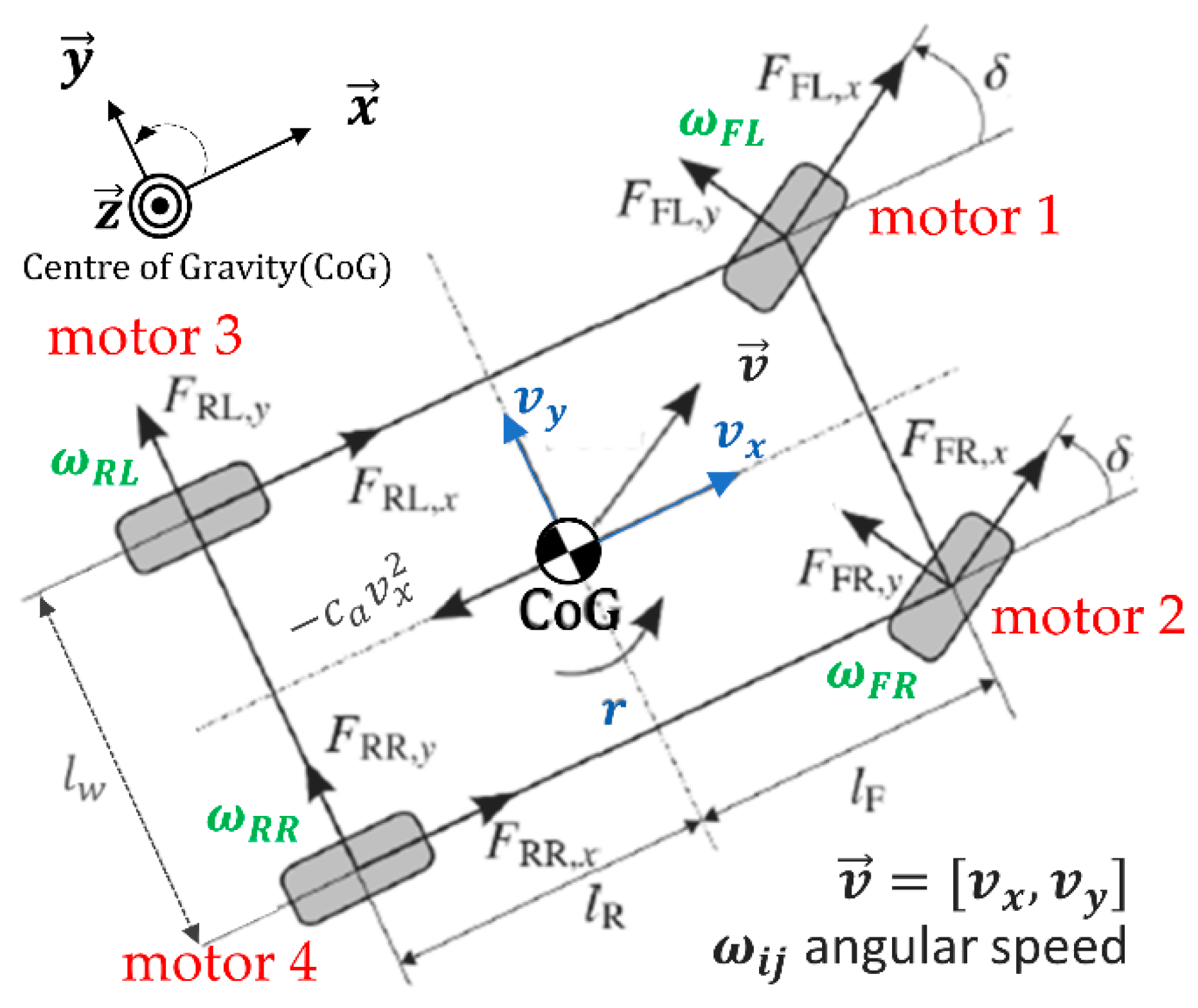
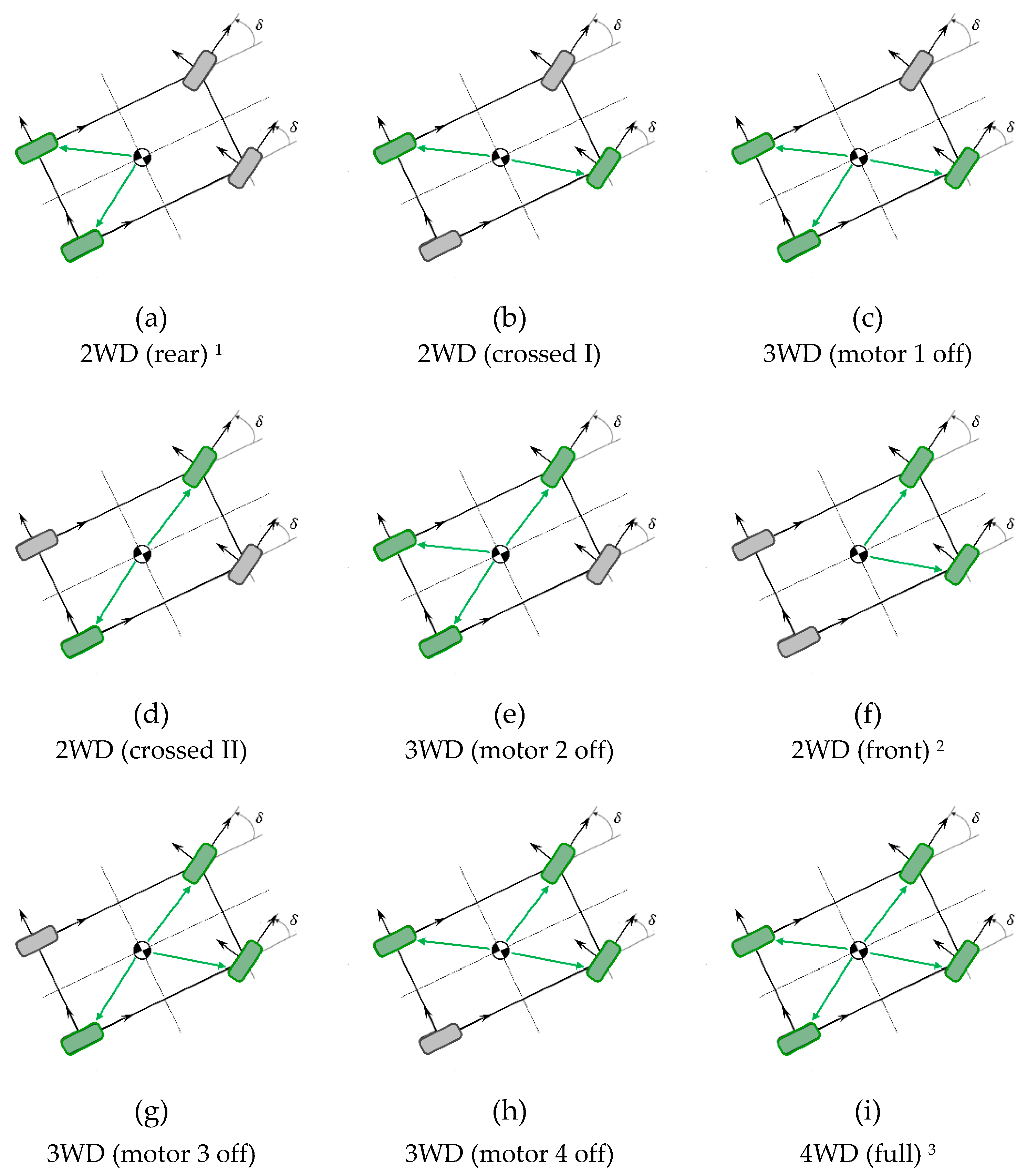
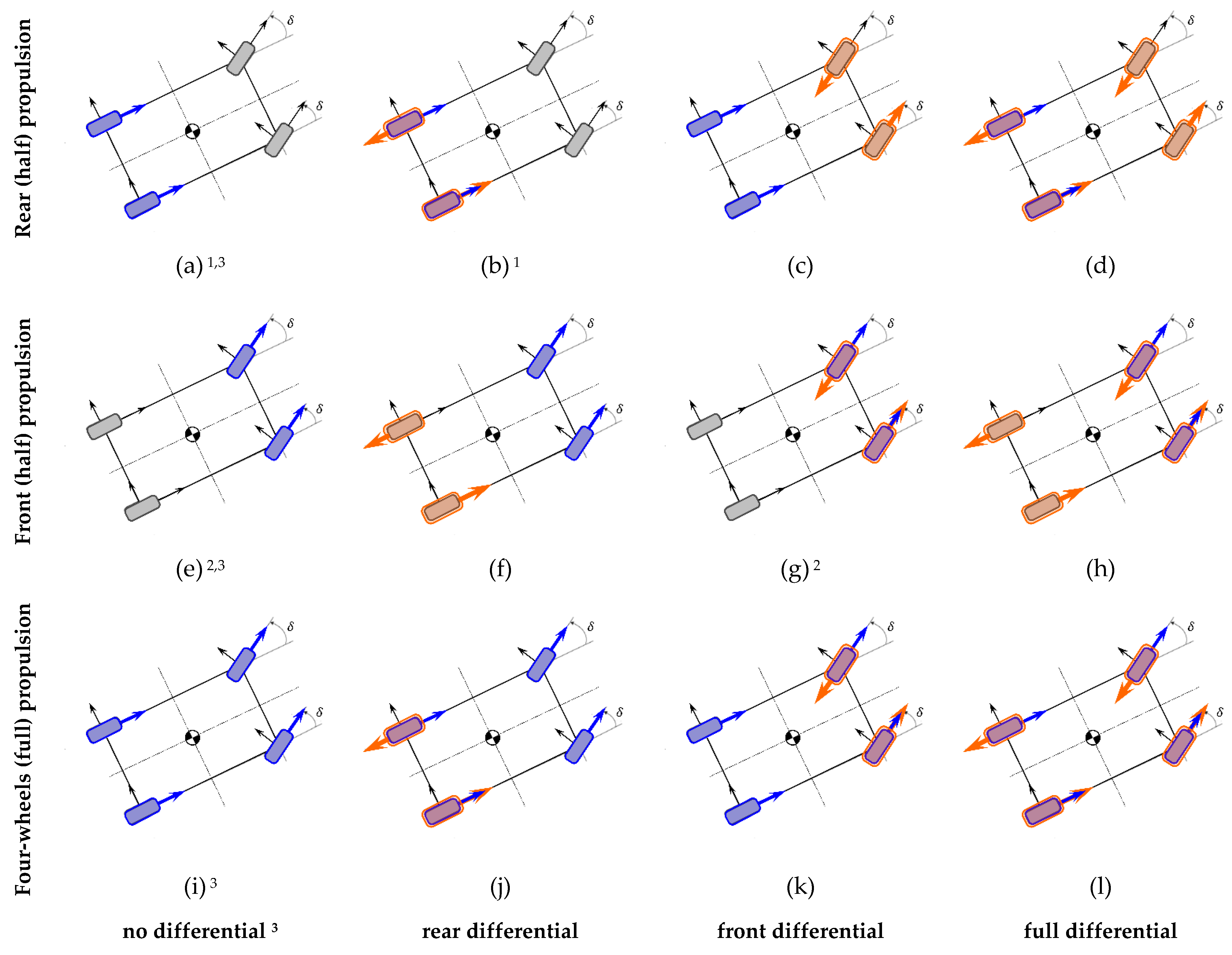
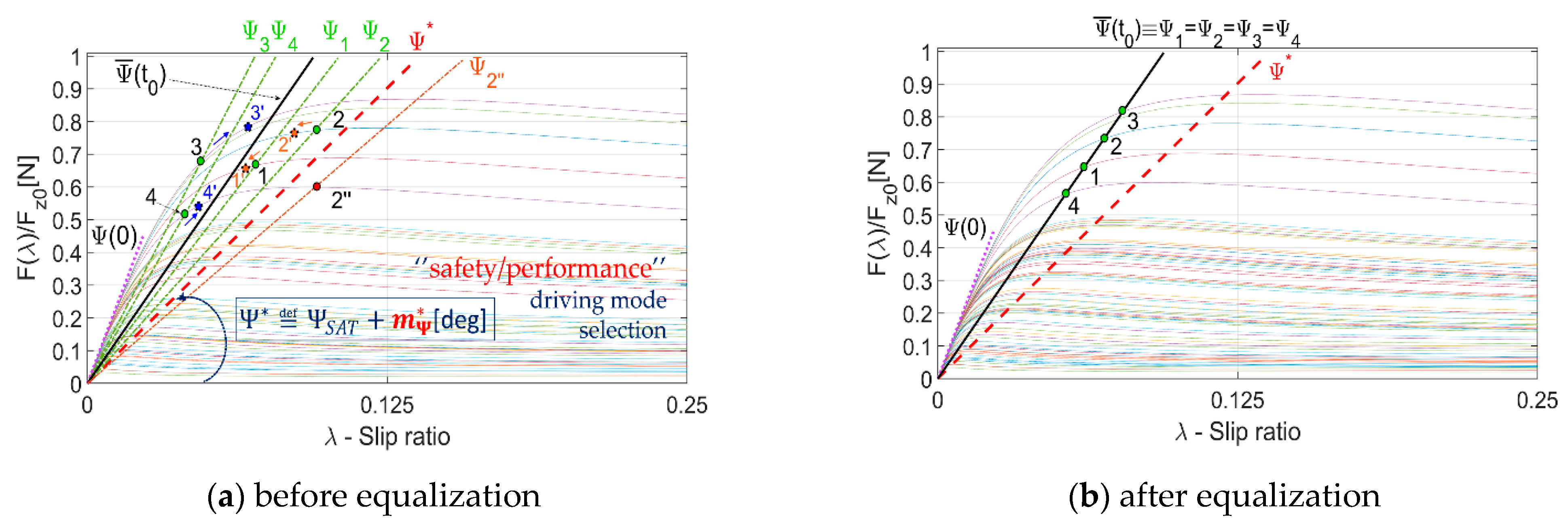
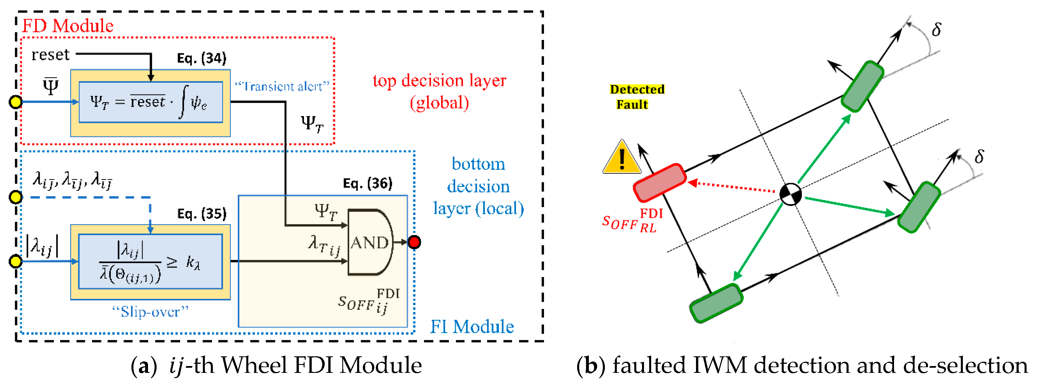
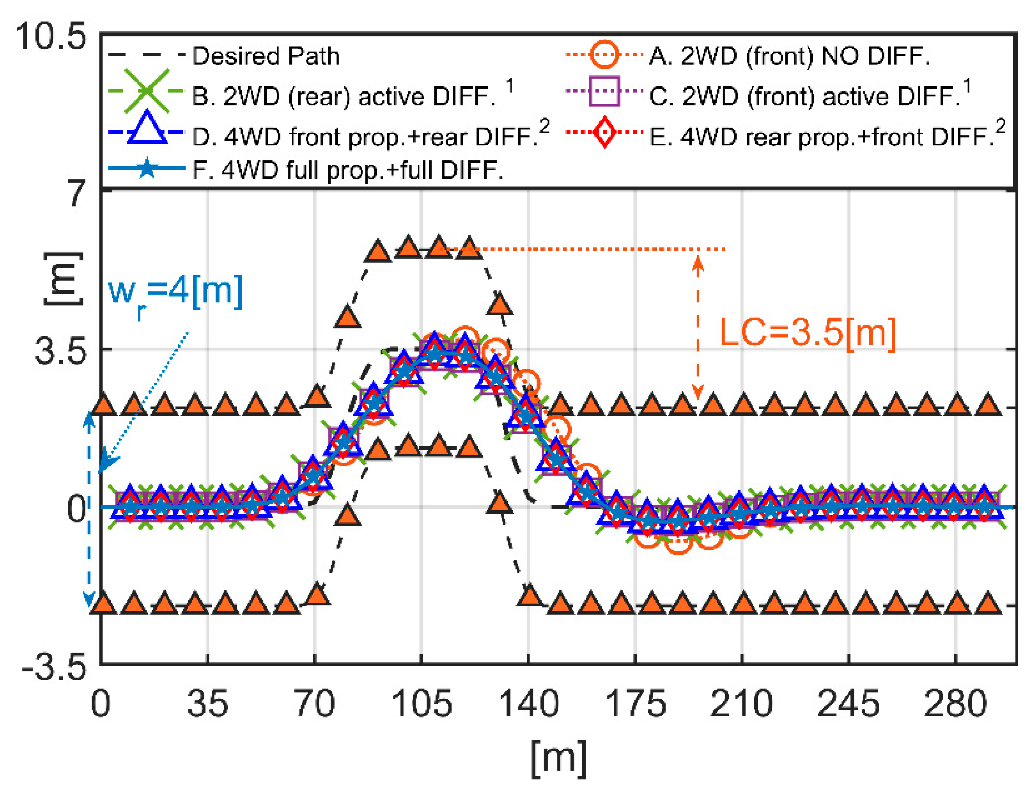
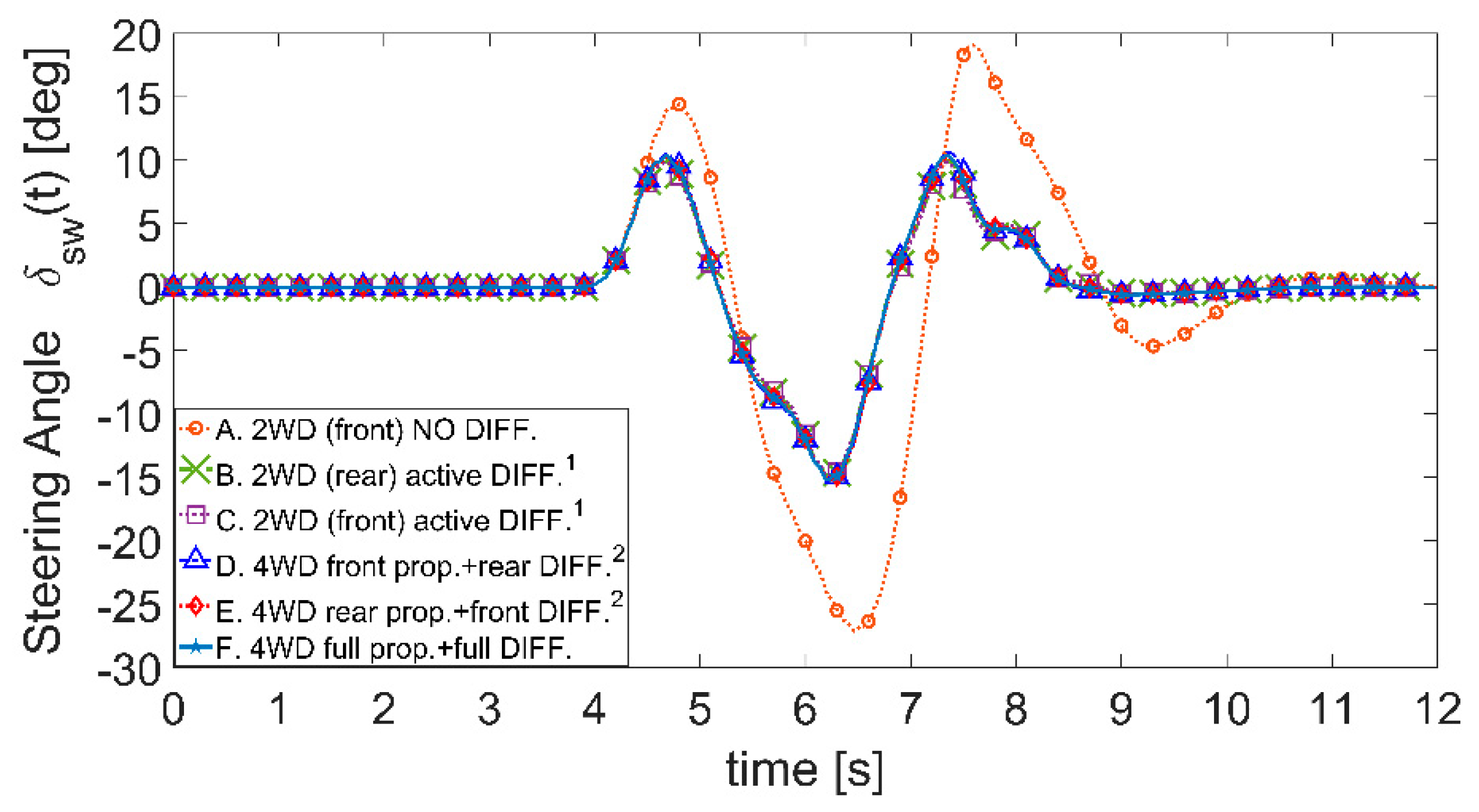
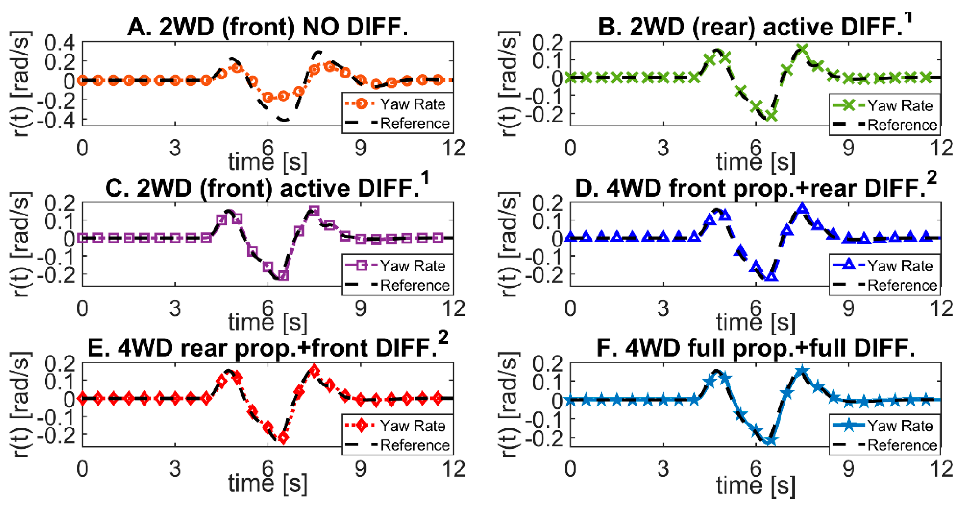
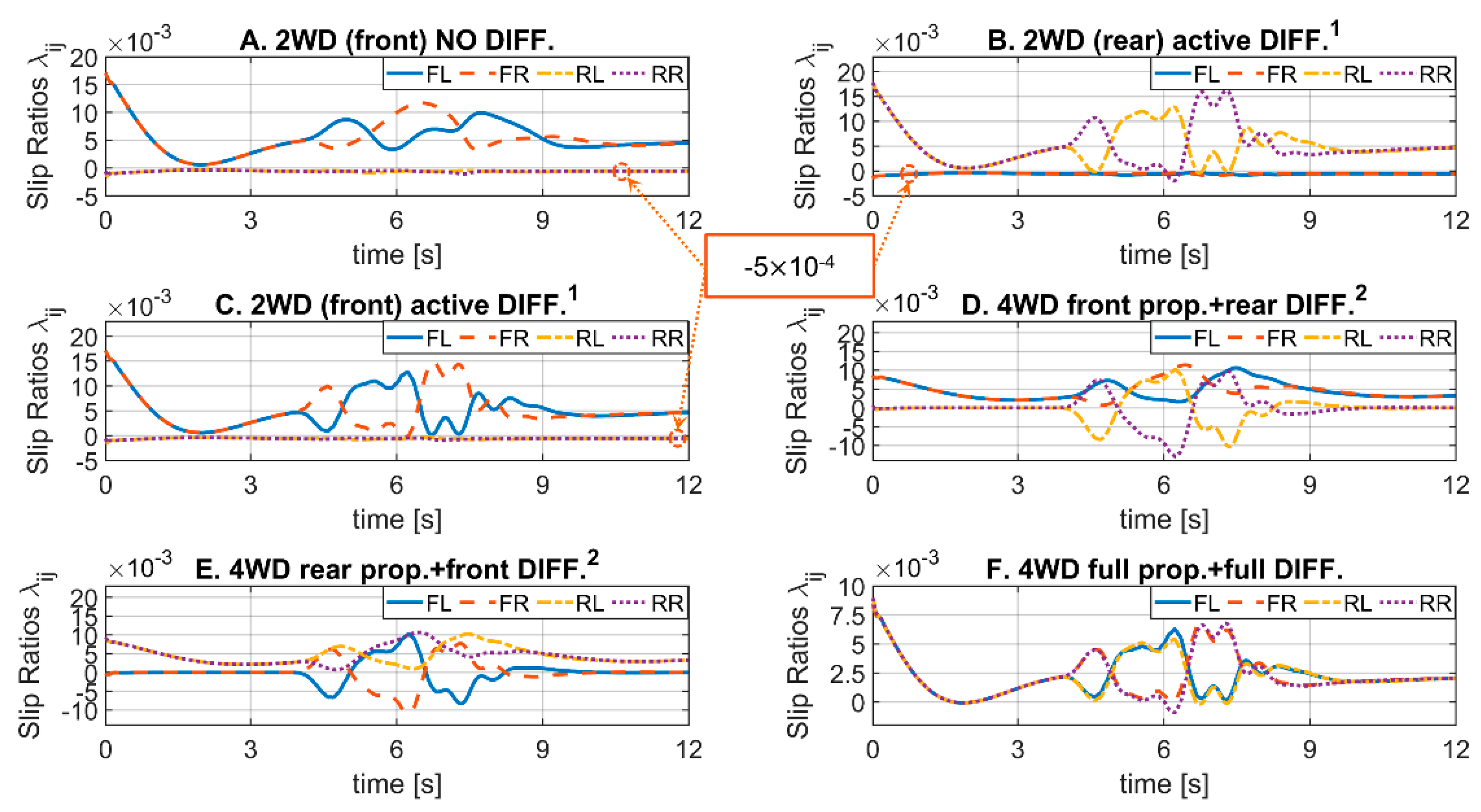
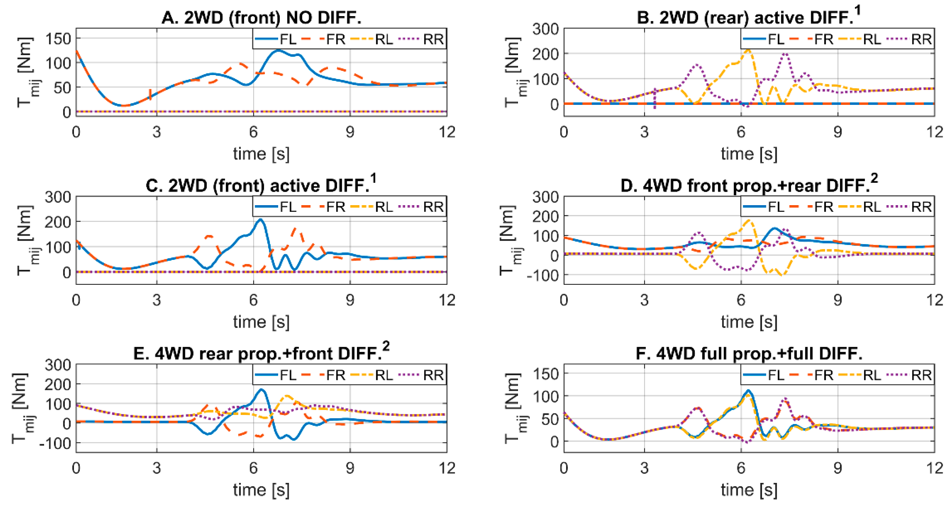
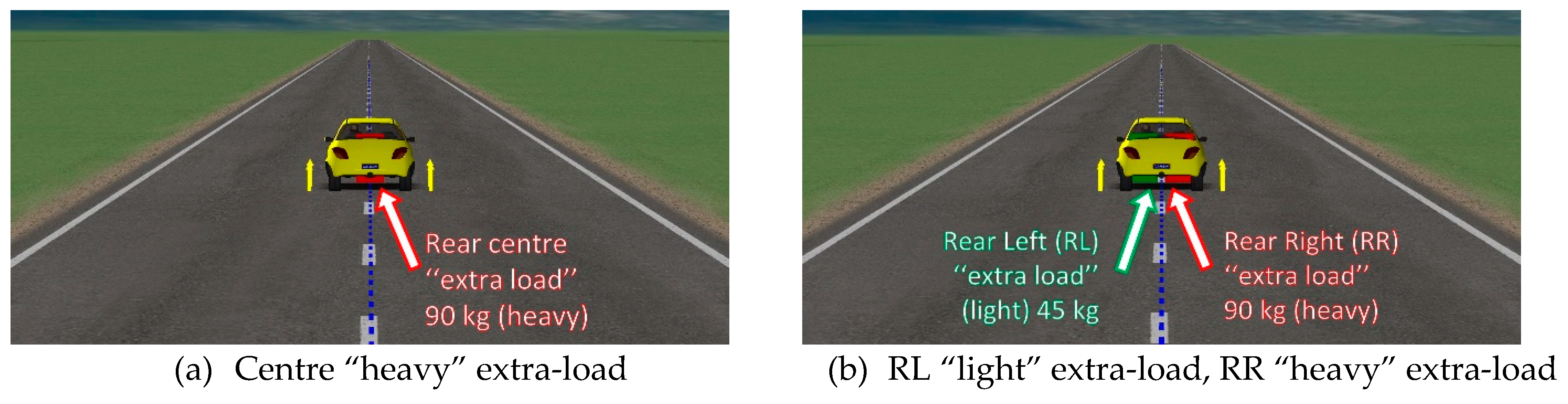
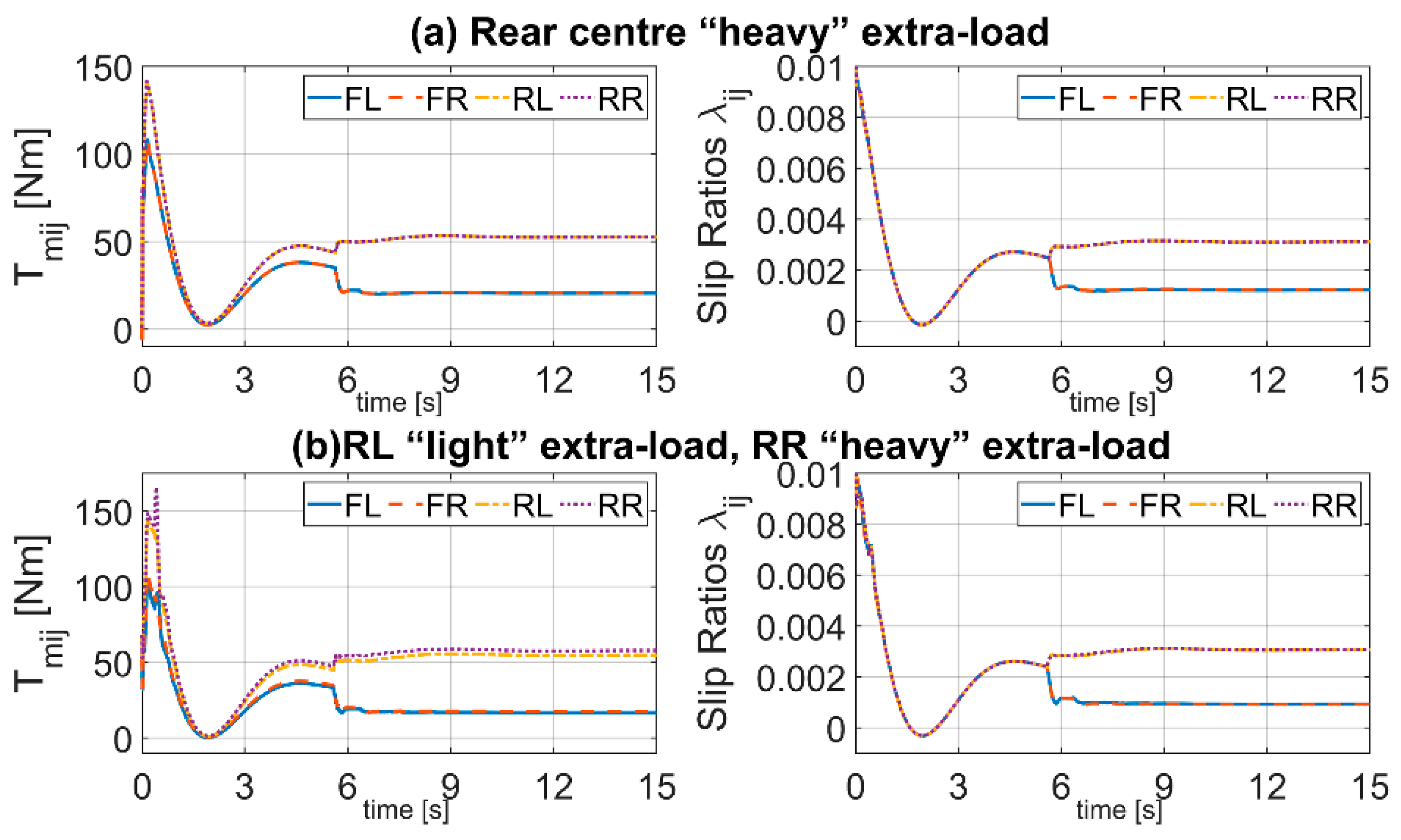
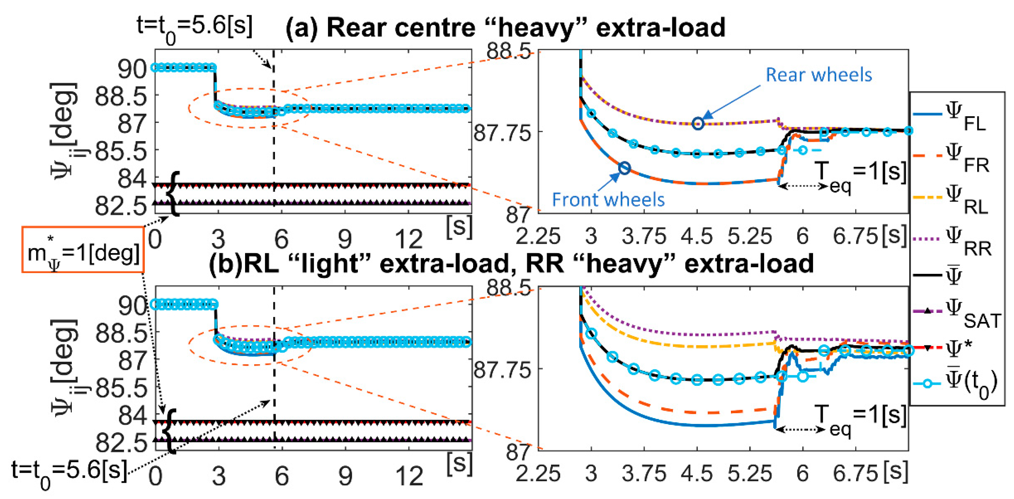
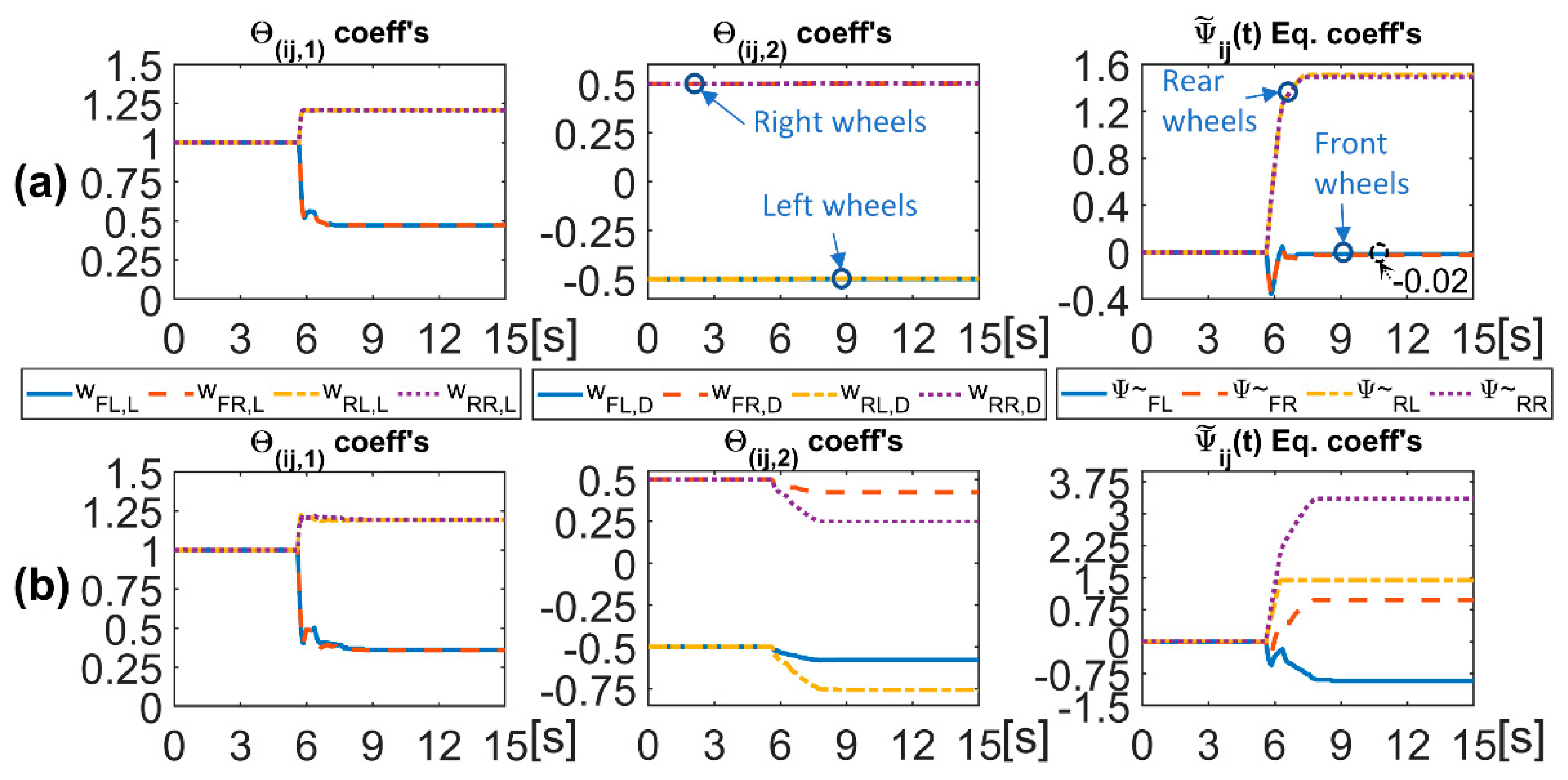
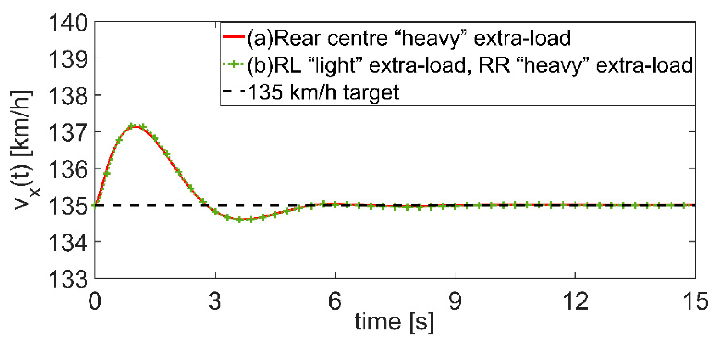
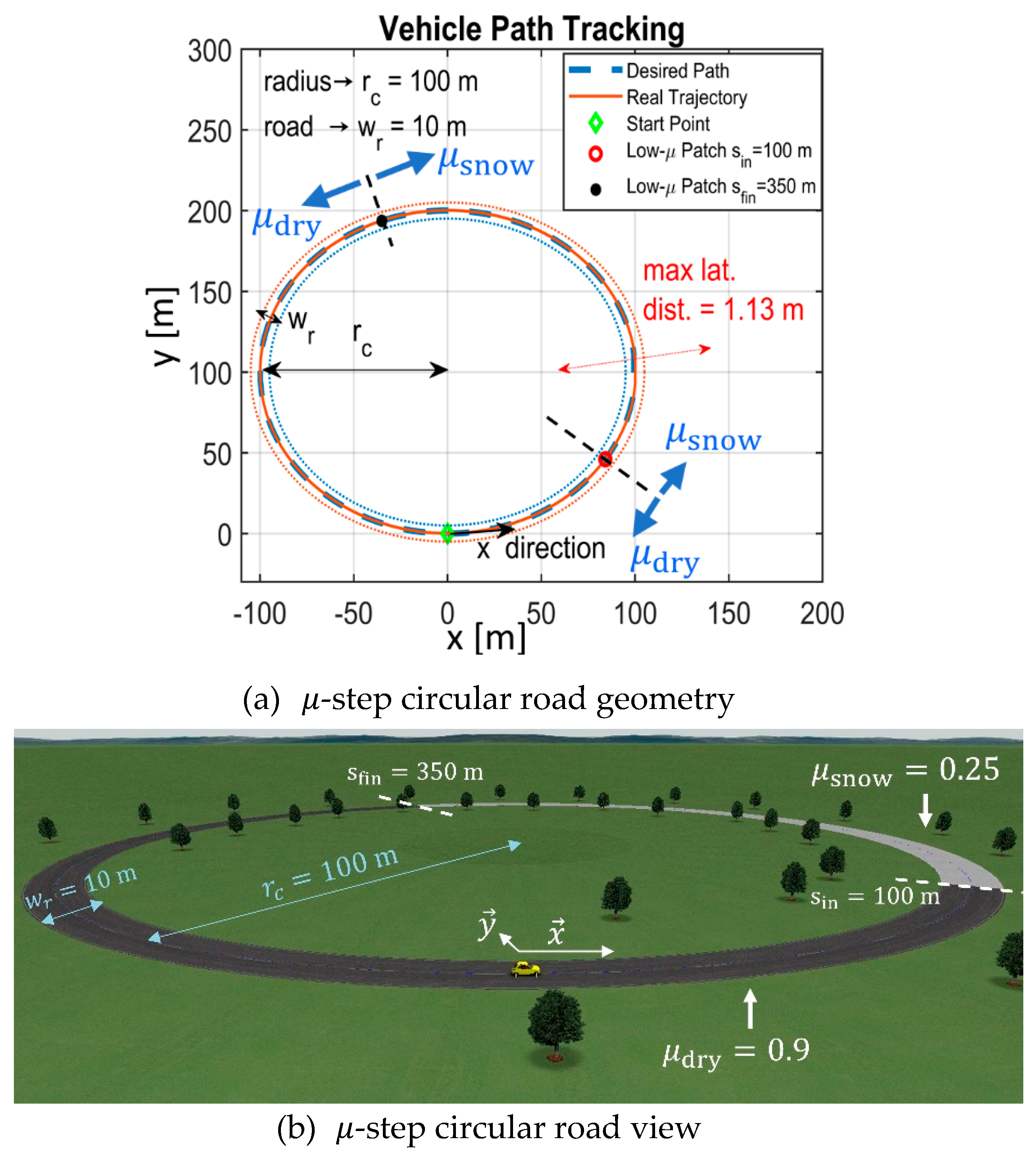
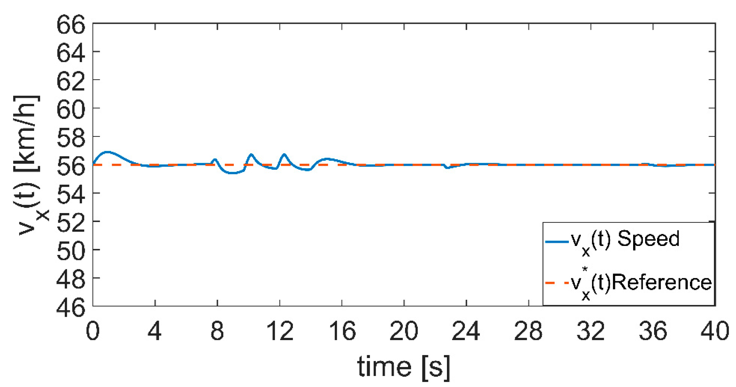
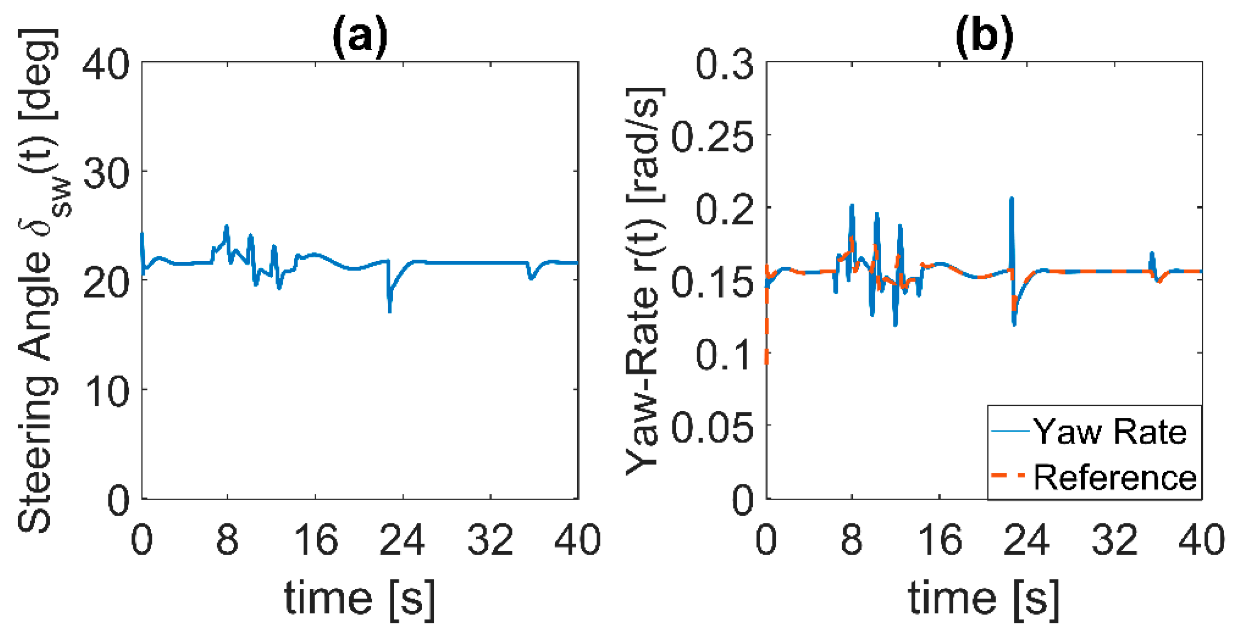
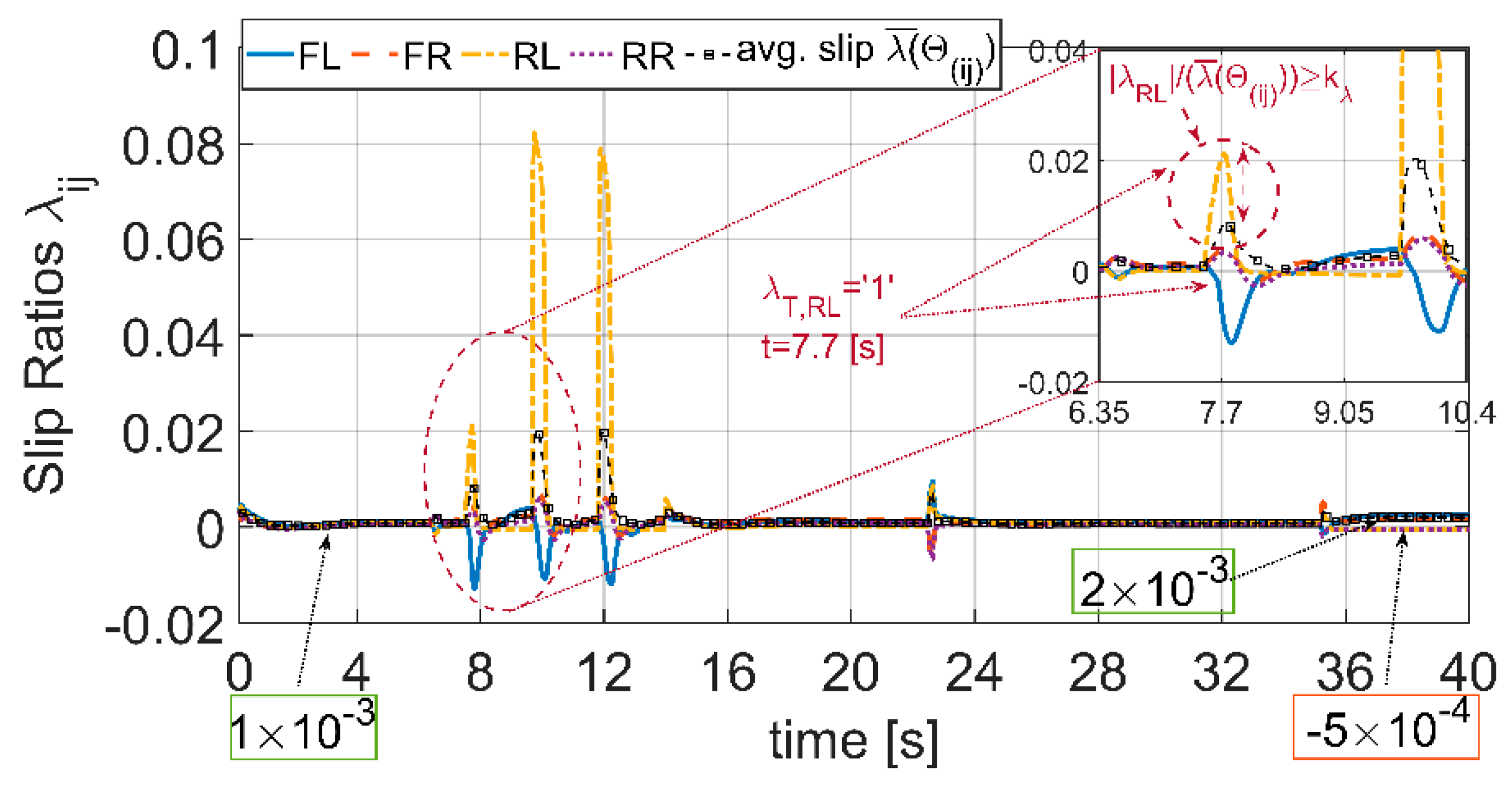
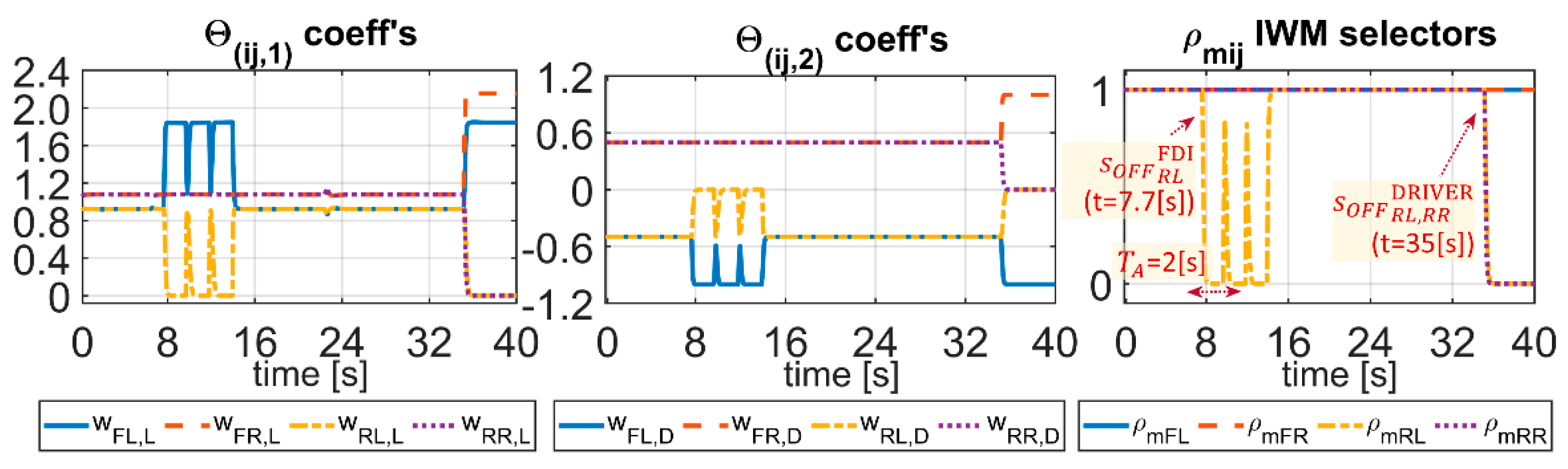
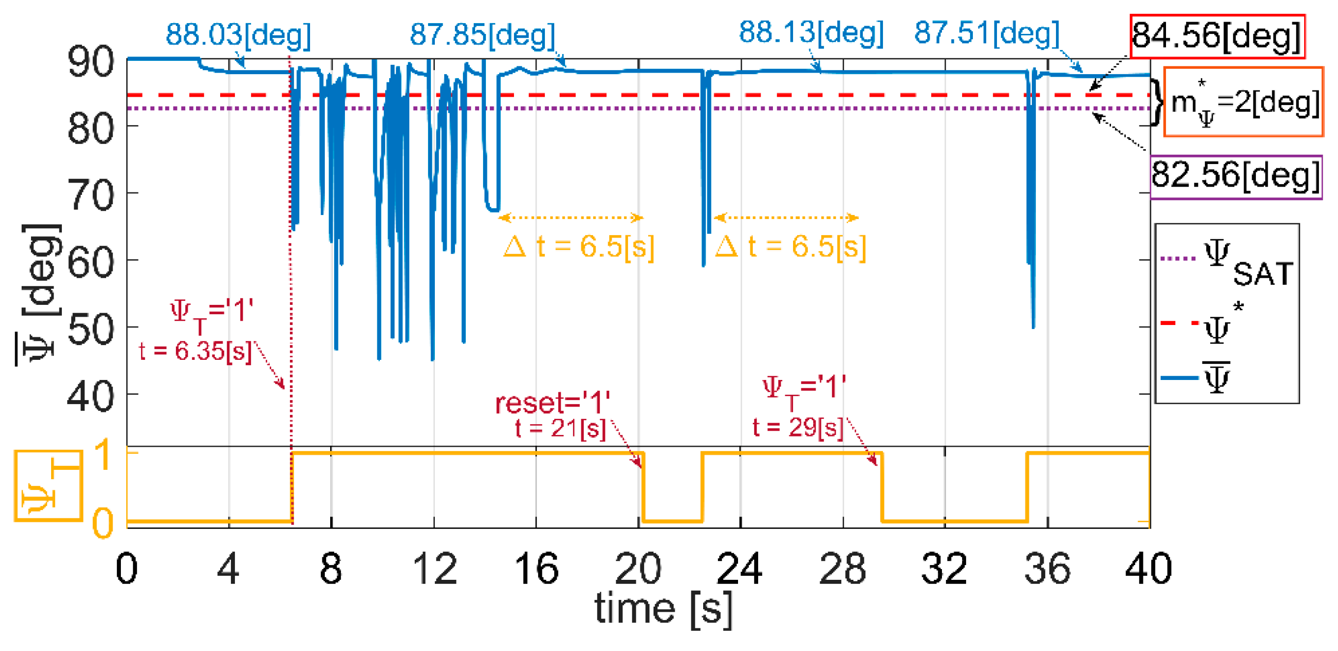
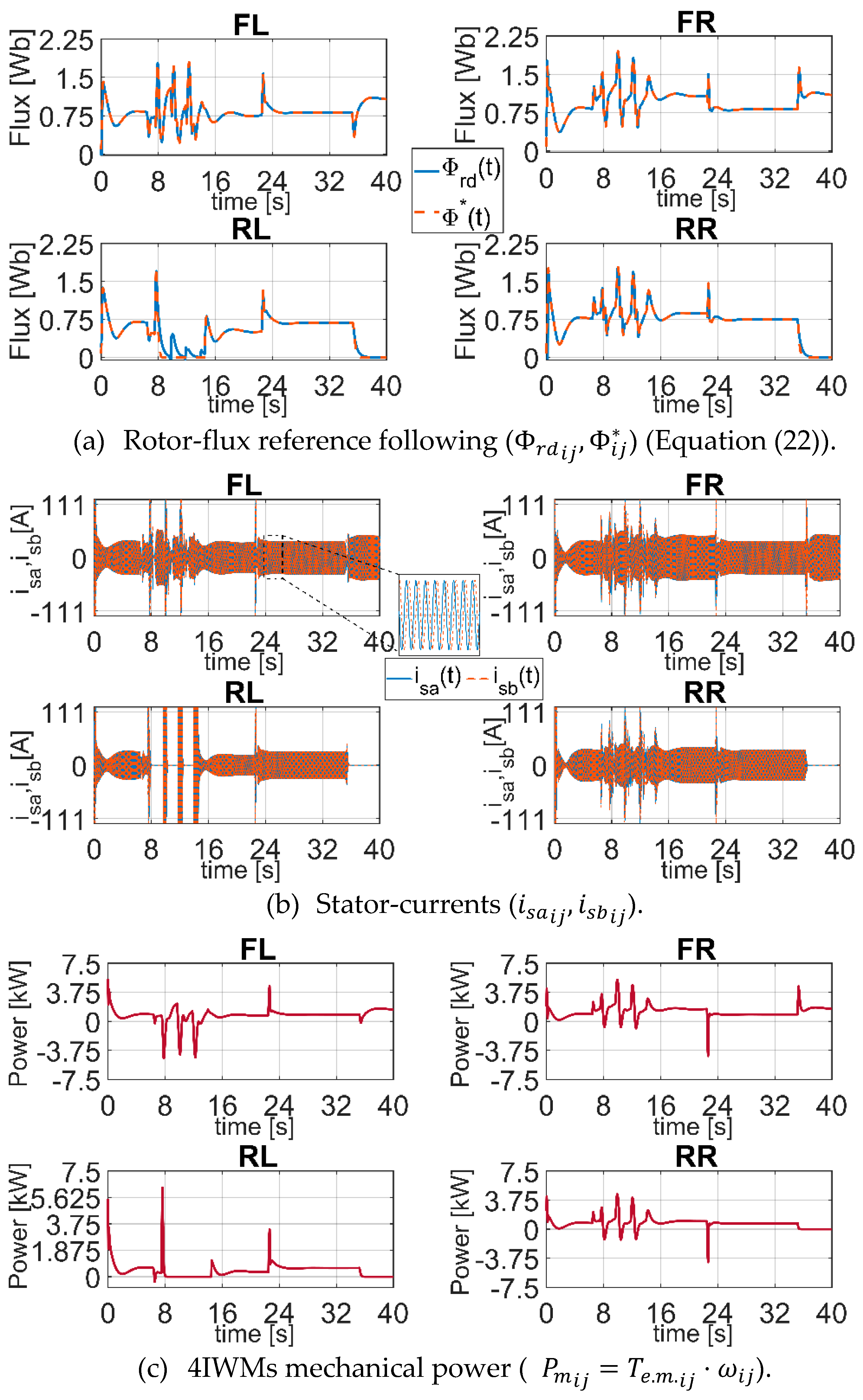
Table 1.
Soft Configuration (Driving Mode Selection) and Hard Configuration: 18 settings.
| REAR propulsion | 1} (0, 1, 0, 0) | no differential | 1–2} | 2WD (rear) | |
| 2} (0,1,0,1) | rear differential | ||||
| 3} (0, 1, 1, 0) | front differential | 13} | 3WD (motor 1 off) | ||
| 14} | 3WD (motor 2 off) | ||||
| 4} | full differential | 15} | 3WD (motor 3 off) | ||
| 16} | 3WD (motor 4 off) | ||||
| FRONT propulsion | 5} | no differential | 5–6} | 2WD (front) | |
| 6} | front differential | ||||
| 7} | rear differential | 17} | 2WD (crossed I) | ||
| 8} | full differential | 18} | 2WD (crossed II) | ||
| 4-WHEELS propulsion | 9} | no differential | 9–12} | 4WD (full) | |
| 10} | rear differential | ||||
| 11} | front differential | ||||
| 12} | full differential | ||||
| [deg] | safety | [deg] | performance | ||
Table 2.
Vehicle, Wheels, IWMs and Control parameters.
| Vehicle | Wheels (Pacejka 5.2) | IWM [10] 1 (37 kW, 50 Hz, 111 A) | |||
| 1005 [kg] | 20.75 [kg] | 23 [kg] | |||
| 750 [kgm−2] | 1.177 [kgm−2] | 0.255 [kgm−2] | |||
| 1.10 [m] | 0.298 [m] | (29.1, 29.1) [mH] | |||
| 1.25 [m] | (1.62, 0.50, 19.4) | 85.1 [mΩ] | |||
| 1.39 [m] | 4100 [N] | 68.5 [mΩ] | |||
| Control parameters | |||||
| PI gains (14)–(21),(37)–(38) | SV Equalization (29), (33) | FDI-switching (27)–(28), (31), (34)–(36) | |||
| (−1.56, −750)103 | (0.85, 0.101) | 0.175 [s] | |||
| −10 | (0.282, 0.321) [g’s] | 2 [s] | |||
| (−0.39, −0.4) | (−40, 0.05 [%]) | 2.5 | |||
| (−5.62, −42.13) | 50 [ms] | 82.56 [deg] | |||
1 {, }.
Publisher’s Note: MDPI stays neutral with regard to jurisdictional claims in published maps and institutional affiliations. |
© 2021 by the authors. Licensee MDPI, Basel, Switzerland. This article is an open access article distributed under the terms and conditions of the Creative Commons Attribution (CC BY) license (https://creativecommons.org/licenses/by/4.0/).
Share and Cite
MDPI and ACS Style
Amato, G.; Marino, R. Reconfigurable Slip Vectoring Control in Four In-Wheel Drive Electric Vehicles. Actuators 2021, 10, 157. https://0-doi-org.brum.beds.ac.uk/10.3390/act10070157
AMA Style
Amato G, Marino R. Reconfigurable Slip Vectoring Control in Four In-Wheel Drive Electric Vehicles. Actuators. 2021; 10(7):157. https://0-doi-org.brum.beds.ac.uk/10.3390/act10070157
Chicago/Turabian StyleAmato, Gerardo, and Riccardo Marino. 2021. "Reconfigurable Slip Vectoring Control in Four In-Wheel Drive Electric Vehicles" Actuators 10, no. 7: 157. https://0-doi-org.brum.beds.ac.uk/10.3390/act10070157
Note that from the first issue of 2016, this journal uses article numbers instead of page numbers. See further details here.