DLR TAU-Code uRANS Turbofan Modeling for Aircraft Aerodynamics Investigations †


Institute of Aerodynamics and Flow Technology, DLR, 38108 Braunschweig, Germany
†
This paper is an extended version of my paper published in AIAA Scitech 2019 Forum, San Diego, CA, USA, 7–11 January 2019.
Aerospace 2019, 6(11), 121; https://0-doi-org.brum.beds.ac.uk/10.3390/aerospace6110121
Submission received: 27 September 2019
/
Revised: 29 October 2019
/
Accepted: 30 October 2019
/
Published: 3 November 2019
(This article belongs to the Special Issue Progress in Jet Engine Technology)
Abstract
:In the context of an increased focus on fuel efficiency and environmental impact, turbofan engine developments continue towards larger bypass ratio engine designs, with Ultra-High Bypass Ratio (UHBR) engines becoming a likely power plant option for future commercial transport aircraft. These engines promise low specific fuel consumption at the engine level, but the resulting size of the nacelle poses challenges in terms of the installation on the airframe. Thus, their integration on an aircraft requires careful consideration of complex engine–airframe interactions impacting performance, aeroelastics and aeroacoustics on both the airframe and the engine sides. As a partner in the EU funded Clean Sky 2 project ASPIRE, the DLR Institute of Aerodynamics and Flow Technology is contributing to an investigation of numerical analysis approaches, which draws on a generic representative UHBR engine configuration specifically designed in the frame of the project. In the present paper, project results are discussed, which aimed at demonstrating the suitability and accuracy of an unsteady RANS-based engine modeling approach in the context of external aerodynamics focused CFD simulations with the DLR TAU-Code. For this high-fidelity approach with a geometrically fully modeled fan stage, an in-depth study on spatial and temporal resolution requirements was performed, and the results were compared with simpler methods using classical engine boundary conditions. The primary aim is to identify the capabilities and shortcomings of these modeling approaches, and to develop a best-practice for the uRANS simulations as well as determine the best application scenarios.
1. Introduction
Increasing environmental and economic requirements continue to drive turbofan engine development towards larger bypass ratio engine designs, with so-called Ultra-High Bypass Ratio (UHBR) engines a likely power plant choice for future commercial transport aircraft. These engines promise low specific fuel consumption at the engine level, but the resulting size of the nacelle poses challenges in terms of the installation on the airframe. Thus, their integration on an aircraft requires careful consideration of complex engine–airframe interactions impacting performance, aeroelastics and aeroacoustics on both the airframe and the engine sides.
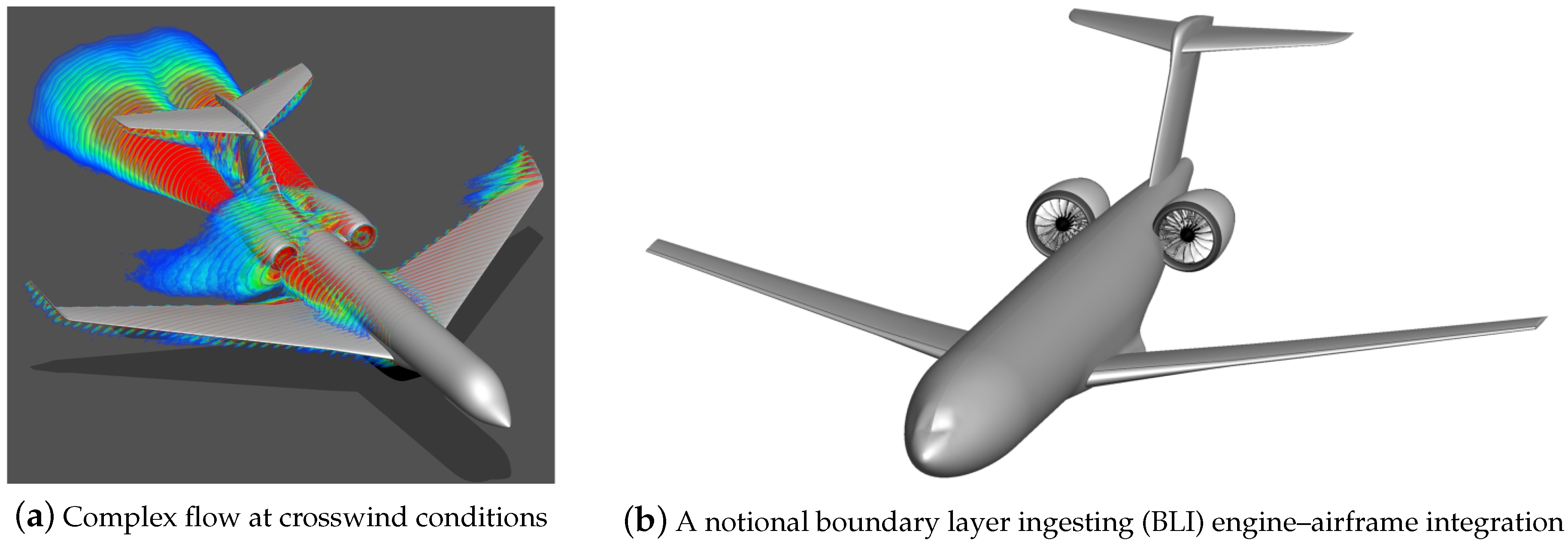
In the frame of the EU funded Clean Sky 2 project ASPIRE, the DLR Institute of Aerodynamics and Flow Technology is contributing to an investigation of numerical analysis approaches for the aerodynamic, aeroacoustic and aeroelastic study of UHBR engines. A particular focus is the assessment of turbofan engine CFD modeling approaches in external aerodynamics focused studies using the DLR TAU-Code [1]. As highlighted in Figure 1, several current research topics show that there are some unique configurations or operating scenarios, where strong mutual interaction between the airframe aerodynamics and the engine, in particular the fan module, flowfield occur. In some of these cases, a high fidelity modeling of the fan may be necessary in the airframe CFD studies to account for these interactions. For example, as shown for a representative business jet configuration in Figure 1a, the fan is subject to an extremely perturbed vortical flowfield coming form the airframe at take-off conditions under strong crosswind. Furthermore, the promise of improved system level fuel burn offered by the integration of engines in a boundary layer ingesting (BLI) configuration on the aircraft, as shown for a notional configuration in Figure 1b, clearly also has strong implications to assess both fan and airframe aerodynamics in a more integrated study than typically done today.
Beyond these specific cases, the requirement to keep nacelle weight and wetted areas down while moving to larger bypass ratios will also result in shorter nacelle inlet lengths. This will also directly result in stronger airframe induced perturbations affecting the fan, pointing to the need for a coupled assessment of airframe and fan aerodynamics and their interactions. To better account for the fan aerodynamic interactions with the external aerodynamic flowfields around the aircraft for these increasingly more complex engine–airframe integration scenarios, the need to employ higher-fidelity fan modeling approaches than the classical engine boundary condition used in typical aerodynamic assessment of the entire configuration has been a growing focus in research projects and industrial applications. The main focus has been on developing simulation strategies accounting for the fan using actuator disc or body force models as well as the full geometric modeling of the low-pressure system of the turbofan in full annulus uRANS CFD analyses [2,3,4,5,6,7].
To understand the best modeling approaches for the engine fan module available in the DLR-developed TAU-Code, in particular when studying some of these challenging airframe aerodynamic topics, a comparison of a classical engine boundary condition and a high-fidelity rotating fan unsteady approach is being done based on a generic isolated UHBR engine configuration. The main focus in this article is a detailed study of various aspects of the uRANS simulation approach, such as spatial and temporal resolution, and their impact on the accuracy of engine performance predictions and important mean and unsteady aerodynamic effects. Furthermore, an evaluation of the impact of the non-conservative nature of the TAU-Codes Chimera technique on mass flow conservation through the engine is presented, to demonstrate sufficient accuracy for the intended applications scenarios.
The uRANS modeling method developed using these simpler isolated engine studies are expected to be directly applicable to future complex integrated engine–airframe configuration studies, such as those shown in Figure 1. With concurrent studies looking into the use of actuator disc and body force models, the overall aim of this and future work is to identify the capabilities and short-comings of each model, develop a best-practice approach in each case and determine the best application scenarios.
2. Geometry and Test Case Definition
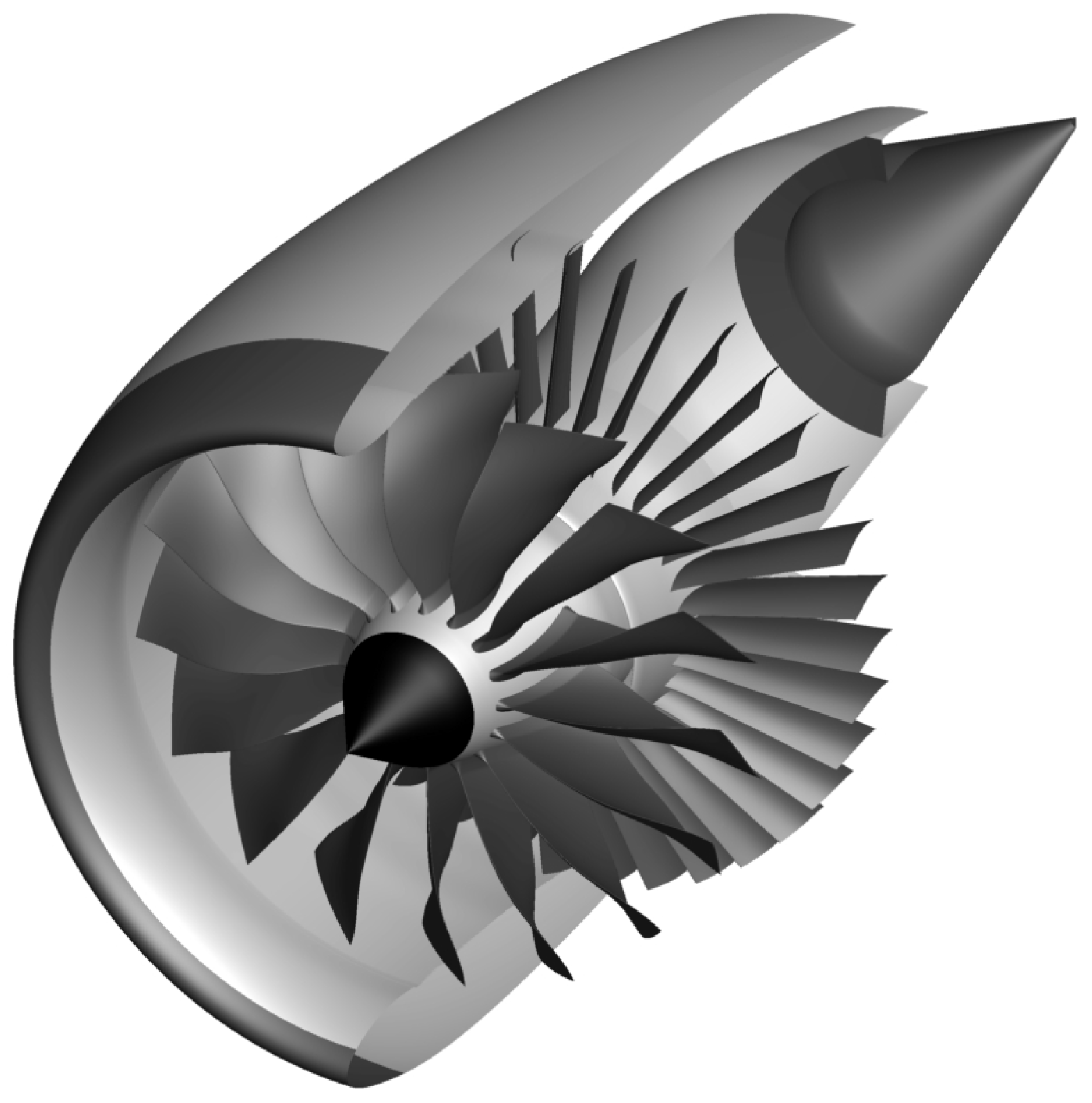
The isolated UHBR engine studied in this paper and shown in Figure 2 was designed within the EU Clean Sky 2 research project ASPIRE as a generic engine for numerical studies and is representative of a modern UHBR turbofan [2,3]. The nacelle shape was supplied by Airbus, while the fan stage, designed for application in a geared turbofan type engine with a low pressure ratio and a 16:1 bypass ratio, was designed by the DLR Institute of Propulsion Technology [8]. It consists of 16 blades in the fan and 36 OGVs in the bypass duct. The nacelle features an inlet with a droop angle and a small length-to-diameter ratio. In the engine design, the use of three different bypass nozzles, differing in the throat area, was foreseen to ensure a sufficient surge margin for the ultra-high bypass ratio fan is achievable at all operating conditions. The test cases reported in this article all feature the identical intermediate nozzle area design.
Presently, the investigations have focused on four engine operating points, a subset of those that were defined in the frame of the project. They are the take-off points Sideline (SID), Buzz-Saw Noise (BSN) and Cutback (CUT) as well as the Approach (APP) point, which are reference points for the noise certification of an aircraft. Therein, the Cutback point is defined as the noise measured at a distance of 6500 m from the start of the take-off roll, directly under the airplane; the Sideline point specifies a noise measurement 450 m from the runway centerline at a point where the noise level after liftoff is greatest; and the Approach point is also defined as a measurement under the airplane when it is at a distance of 2000 m from the runway threshold. The Buzz-Saw Noise point is related to the Sideline point, but has the engine producing more thrust due to a higher fan rotational speed, which leads to the blade tips operating at supersonic tip mach numbers.
General specifications for these are listed for reference in Table 1, through the specification of aircraft altitude, flight speed and incidence angle, as well as the fan shaft rotational speed normalized to the design shaft speed at the engines cruise aerodynamic design point (ADP). The incidence angle is the effective inflow angle to the engine inlet, which already takes wing upwash effects into account, with the assumption of the engine being integrated with the aircraft in a typical under-wing installation. In addition, a specification of the core engine operating point was provided in each case in the form of mass flow rates as well as the exhaust gas total temperature and pressure. These specifications allow for the modeling of the mean core engine flow using classical engine boundary conditions.
3. Computational Strategy
All CFD simulations are performed utilizing the DLR TAU-Code for both the steady RANS and the uRANS computations. For the latter, much know-how was transferred from a process chain that has already been successfully applied in a number of recent propeller and CROR investigations [1,9,10,11,12,13,14], where validation with wind tunnel test data has shown high-quality engine performance predictions for various isolated and installed configurations is achievable, with deviations of less than to the experimental values.
3.1. DLR TAU-Code CFD Simulations
The DLR TAU-code [15] is an unstructured finite-volume vertex-based CFD solver developed by DLR. For the RANS and uRANS simulations described here, spatial discretization of the convective fluxes is done using a second-order central differencing scheme with scalar dissipation while the viscous fluxes are discretized with central differences [16]. Turbulence in these fully turbulent simulations is modeled with the one-equation model of Spalart and Allmaras [17,18]. The well-established dual time approach is used in the DLR TAU-code to compute the unsteady flow of the full annulus rotating fan cases in this study [19]. For each discrete physical time step, a solution is obtained through a time-stepping procedure in a pseudo-time making use of the same convergence acceleration techniques used for steady-state computations, namely a lower-upper symmetric Gauss-Seidel (LU-SGS) implicit relaxation scheme, local time stepping, multigrid and residual smoothing [20,21]. To simulate the relative motion of the rotors, use is made of the codes Chimera capability as well as the implemented motion libraries [22,23,24,25].
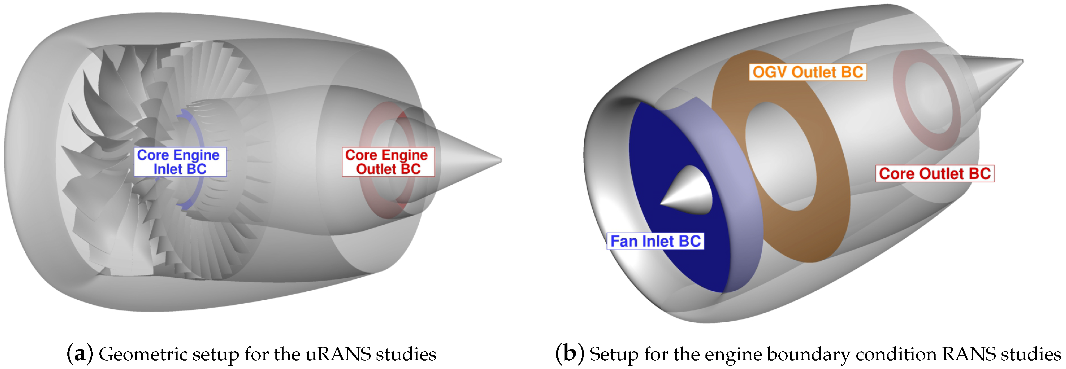
Figure 3 shows the CFD modeling approach used in the present study. For the uRANS studies, the rotor and stator are fully geometrically modeled, with an engine boundary condition setup used for the core in- and outlet, as shown in Figure 3a. For the RANS studies with engine boundary conditions, the fan stage effect is modeled, as plotted in Figure 3b, through the use of a planar surface at the position of the fan and an outlet plane located just downstream of the OGVs in the bypass duct. As implemented in the DLR TAU-Code, the engine boundary conditions require a specification of total pressures and total temperatures, or alternatively a target mass flow rate and the total temperatures at the exit planes of the core or fan stage. A coupling procedure is then used, which iterates the core and/or fan inflow plane static pressure in order to achieve a mass flow rate that equals that at the core and/or fan exhaust. Again, as an alternative, the target mass flow rate can be specified, which is then achieved in the course of the simulation through a fan plane static pressure iteration procedure. The core engine settings were specified in terms of the target mass flows and the exhaust total temperatures in both the RANS and uRANS simulations. To model the fan flow in the RANS simulations using the engine boundary condition, the pressure and temperature at the fan stage outlet were set according to the engine model specifications supplied by Airbus. The fan inlet boundary was coupled to the fan and core exhausts, resulting in an iterative achievement of the sum of bypass and core mass flows at the fan face.
3.2. Mesh Generation
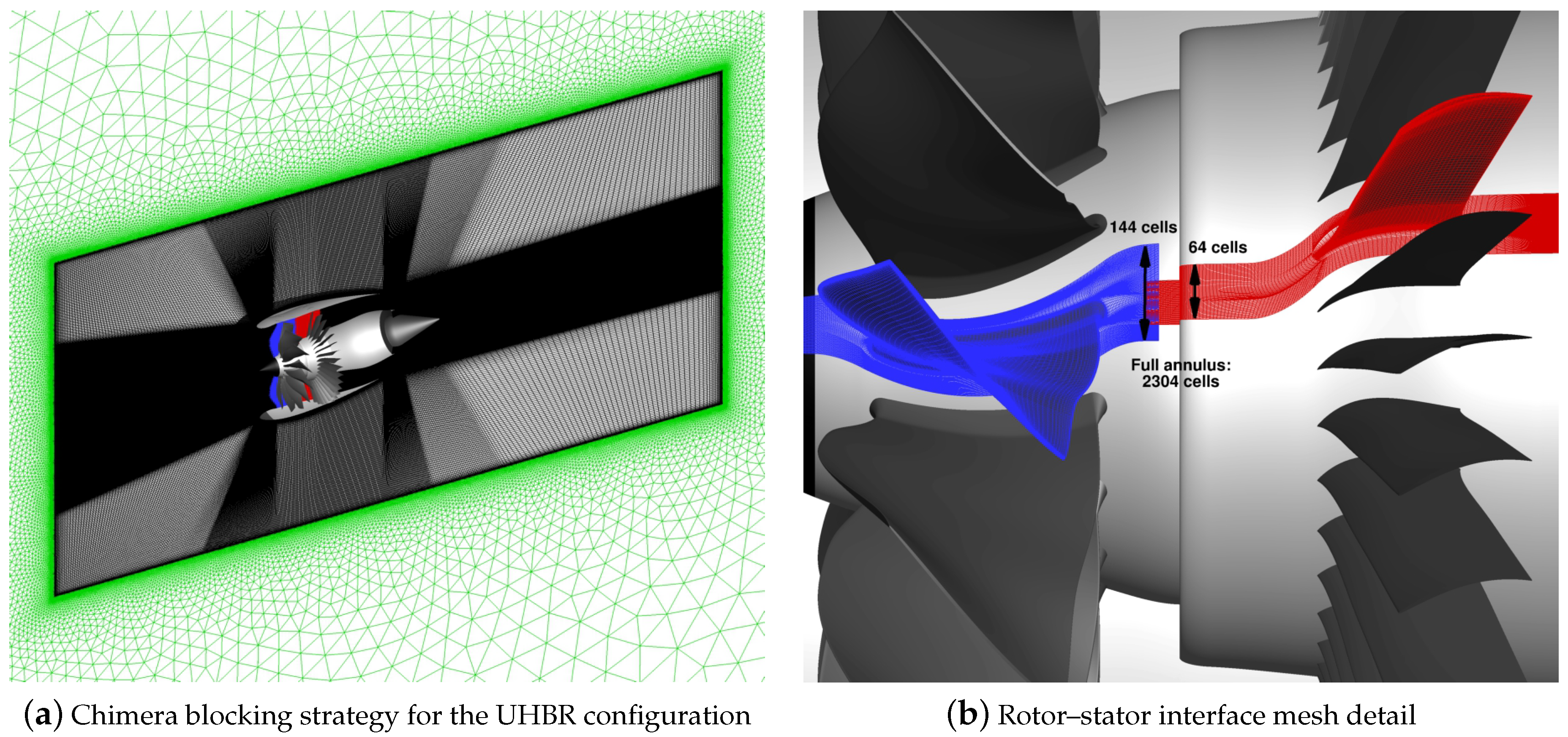
For the UHBR simulations, the flexibility afforded by the Chimera approach was exploited and meshes consisting of four mesh blocks were created, as shown in Figure 4. The first mesh block, a hybrid-unstructured CentaurSoft Centaur generated mesh, is the farfield block, with farfield boundaries located at a distance of at least 25 times the fan diameter from the rotor center in all directions. Embedded in this block is a block-structured nacelle mesh, which in turn features embedded cylindrical mesh blocks for the fan rotor as well as the OGVs. All meshes except the farfield block are block-structured grids generated using the commercial ANSYS ICEM CFD Hexa mesh generation software. A family of meshes was generated, with a coarse, a medium and fine grid, which enables a study of the mesh resolution impact on solution quality. Total mesh size for the isolated UHBR configuration as shown in Figure 4a ranges from nodes for the coarse to nodes for the fine mesh level, with further grid details listed in Table 2.
In addition to ensuring an adequate resolution of boundary layers (including the laminar sublayer) on all surfaces of the engine, with a dimensionless wall distance of achieved throughout, a particular focus of the mesh generation was to ensure the transfer of the fan blade wakes into the OGV mesh block is possible in the uRANS simulation with minimal interpolation losses [12]. Thus, the overlap region of the these two grids is meshed in a way that ensures an identical, axially-aligned cell orientation, and a matching number and uniform spacing of the cells for the annulus on the rear Chimera boundary of the fan block and the forward Chimera boundary of the OGV block. As shown in Figure 4b, for the finest mesh density, the mesh features a total of 2304 cells in azimuthal direction at the rotor–stator interface on either side. For all mesh blocks, the symmetry, axisymmetry or rotationally symmetric nature of the geometry was exploited where possible, ensuring, for example, that each blade of the fan has an identical spatial discretization.
For the engine boundary condition simulation, a single-block hybrid-unstructured mesh with million nodes is used, which is generated using the CentaurSoft Centaur mesh generation software.
3.3. The Simulation Approach
While straightforward steady-state RANS simulations are performed for the studies using the engine boundary conditions, the uRANS computations are initialized with a steady-state simulation in which the rotor remains stationary. This ensures that the nacelle flowfield is already a close approximation of the mean state at the flight condition, which reduces computational times in the unsteady simulation. In the subsequent uRANS simulation, a step-by-step refinement of the time-step size is performed, with the aim of studying the impact of the temporal resolution on the aerodynamic results.
Table 3 lists the various temporal resolutions in terms of the number of time steps per rotor revolution for which solution output is obtained and analyzed. The final and smallest time-step is linked to the mesh resolution at the fan-OGV Chimera interface. It corresponds to a deflection of the rotor for which there is only a one cell relative motion between the fan and OGV blocks. Thus, for the rotor mesh setup as shown in Figure 4b, the highest temporal resolution studied called for 2304 time steps per rotation, i.e., a rotor motion of per physical time step. The computations were run using up to 720 cores of DLRs 13,000-core -cluster in Braunschweig.
The RANS simulations achieved a converged state after a simulation time of around 20 h using 48 compute cores. The uRANS simulations naturally required run times on the order of days to weeks, depending on the number of cores used and the size of the grid. An exhaustive study on the optimal number of cores to be used for the three differently refined meshes in the unsteady computations for the best turn-around times to obtain results is beyond the scope of this article and often limited by real-world constraints such as available computational resources of DLR’s cluster. As a point of reference, however, a physical time step for the coarse mesh uRANS run required a roughly 600 s compute time when using 48 cores, while the corresponding duration for the medium mesh is 800 s using 240 cores and 900 s using 480 cores for the fine mesh case. This means that a full rotor revolution resolved using 360 time steps—which yields good quality mean performance predictions as will be discussed in the subsequent analysis—requires simulation times between two and four days.
4. Aerodynamic Analysis
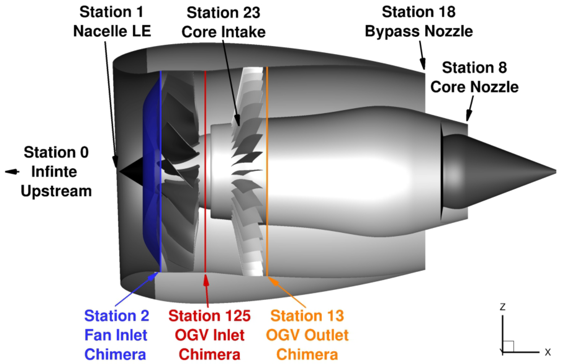
In this section, the results of the various simulation approaches are analyzed in terms of the aerodynamic characteristics and performance. Comparisons are made both with the engine cycle model specifications as well as among the differing fan modeling approaches. Figure 5 shows an overview of the station definitions used in the discussion of the simulation results. The three Chimera interfaces are shown in blue, red and orange, and they generally coincide with locations that are relevant for the performance evaluation of the engine. For example, the evaluation of the fan stage performance, i.e., across both the fan and rotor, draws on the total pressure and temperature results computed in the simulations on the Chimera surfaces located at Station 2 and Station 13. The total mass flow rate of air is evaluated using the Chimera surface at Station 2 and the computed bypass mass flow rate is determined at Station 13. The core engine mass flows are evaluated directly on the planar surfaces which correspond to the previously described boundary conditions definitions, as shown in Figure 3. In general, these latter mass flows are set directly as per the engine cycle model specifications.
The main focus in the discussions is placed on the APP case. This case was chosen as it is one of the more challenging in terms of fan aerodynamics and has relevance for future airframe driven studies, as the interaction of a wing-mounted UHBR engine jet with the high-lift system may be a concern. Results across the full family of mesh densities as well as for the various time steps used are discussed in detail for this case.
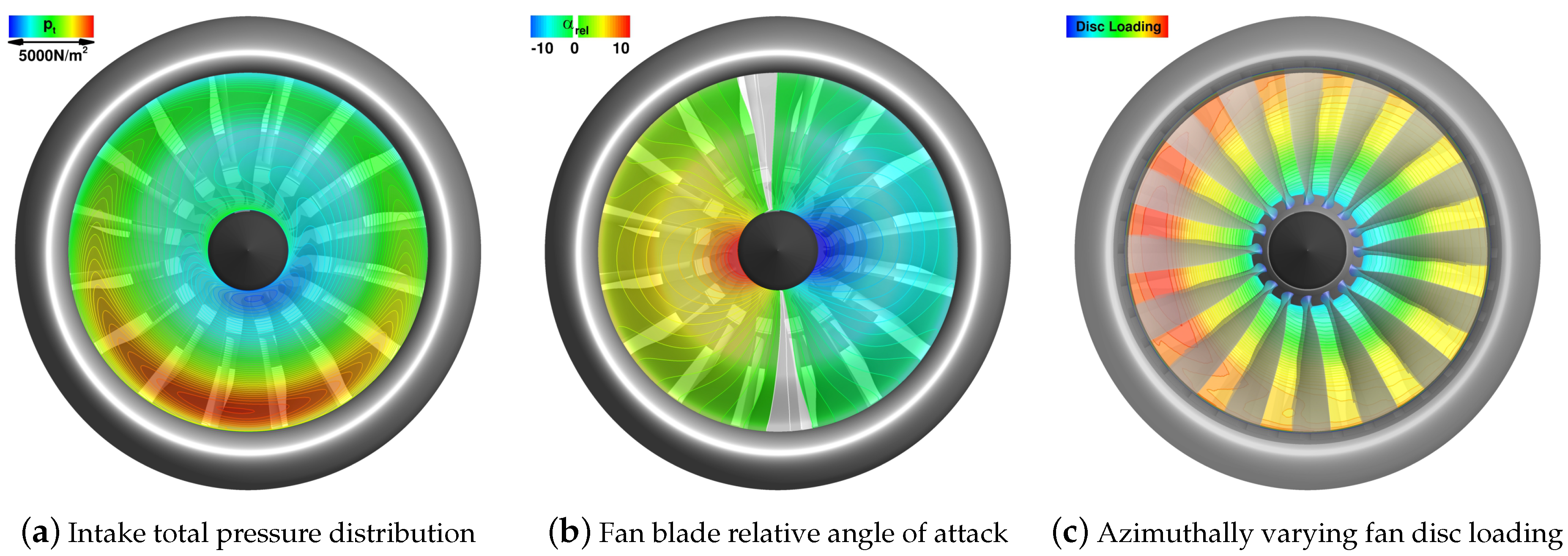
Figure 6 illustrates the impact of the very short intake characteristic of current UHBR nacelle designs on the fan inflow conditions. For the approach condition shown here, which features a high angle of attack of the nacelle, Figure 6a,b highlight, that in a plane just upstream of the fan blade leading edges, a notably perturbed flowfield can be found. The total pressure contours show the effect of the high acceleration of the flow over the short lower lip of the nacelle at the high incidence angle, while the plot of the fan blade effective angle of attack distribution shows that a blade is subject to essentially the nacelle incidence angle across most of its span. For the counter-clockwise fan rotation, this leads to an increasing effective angle of attack for a blade during the downward sweep on the left side and a reduction thereof on the upward sweep on the right side of the nacelle. As a consequence of this, a fan blade is subject to an azimuthally varying inflow, which results in rotor blade loading variations during a rotation. This is shown through the fan rotor disc loading plotted in Figure 6c, and the impacts are discussed in detail in the following section.
4.1. uRANS Simulation Analysis
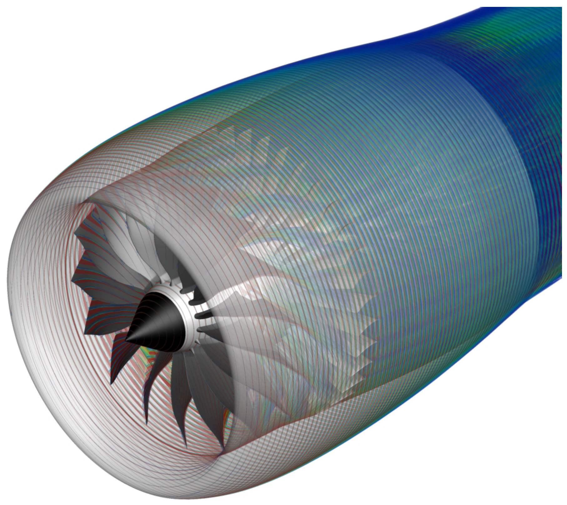
Figure 7 shows an instantaneous result of the uRANS simulation of the UHBR configuration at the approach operating point point using the fine density mesh. The lessons-learned from the previous CROR-studies have been applied and result in a good resolution of the unsteady fan-OGV interactions, as shown in the figure for example through the impingement of the fan blade wakes on the OGV blades. Proper resolution of these dominant unsteady aerodynamic effects is key for potential further exploitation of the uRANS simulations in the frame of structural, aeroelastic or aeroacoustic assessments.
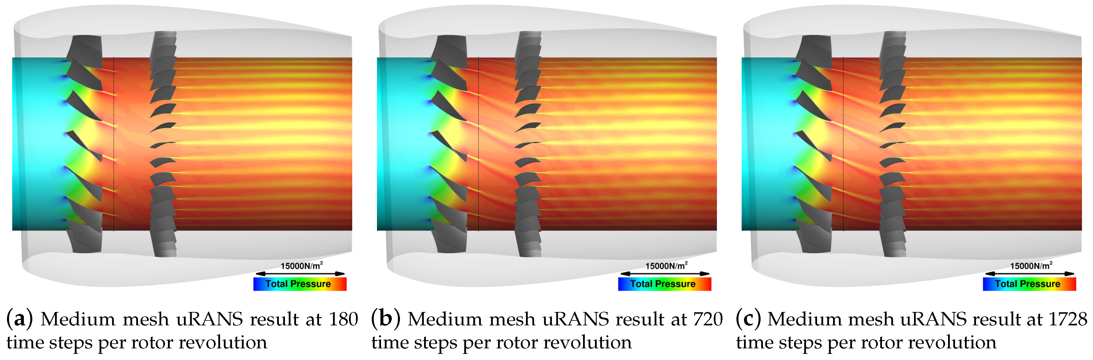
The temporal resolution used in the uRANS analysis has a profound impact on the resolution of the aerodynamic interactions between the fan blades and the OGV vanes. Contour plots of instantaneous solutions taken from the uRANS simulations of the APP case using the medium density mesh at selected time step sizes illustrate this in Figure 8. In each subfigure, total pressure contours are plotted on a cylindrical surface located at a radial position of to show the resolution of the fan blade wakes, in particular as they pass through the Chimera overlap region between the rotating fan and the stationary OGV mesh domain. For the relatively coarse time step size of 180 per revolution, shown in Figure 8a, the significant error introduced in the sustainment of this flow feature, which plays an important role for the unsteady aerodynamic loading on the stator and thus also the fan stage noise, is clearly evident. The successive refinement of the temporal resolution, going to an intermediate value of 720 time steps per rotor revolution in Figure 8b and the to the finest level of 1728 in Figure 8c, shows that using an appropriately small time step size is vital to capture the fan blade wake adequately and ensure its interaction with the outlet guide vanes is properly simulated.
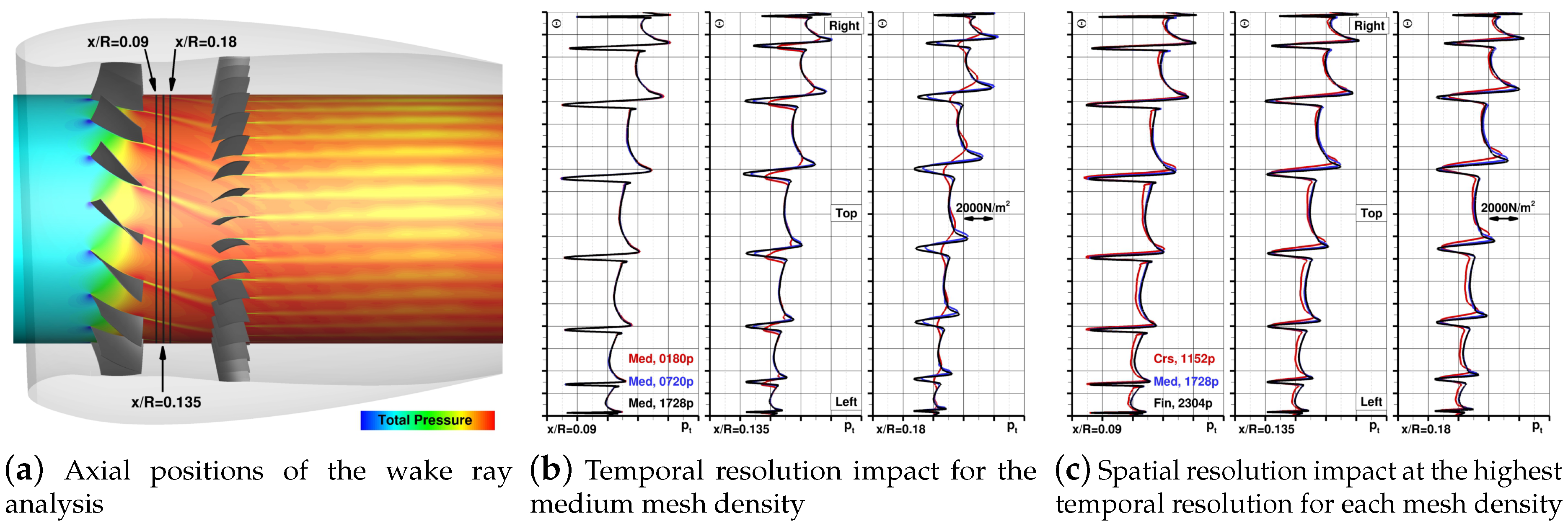
A more quantitative analysis of the temporal resolution and fan blade wake sustainment across the chimera interface is presented in Figure 9. The instantaneous total pressure wake profiles are plotted as a downward look at the engine bypass duct flowfield from above, and show three axial positions denoted using their distance from the fan blade trailing edge at this radial position, as marked in Figure 9a.
The middle plot, Figure 9b, compares the medium mesh uRANS results for the three selected temporal resolutions at an axial location of downstream of the fan blade trailing edge, which is just upstream of the Chimera interface between the rotor and stator mesh domains. Representing a quasi-steady solution in the rotating frame of reference of the fan domain—at least when any temporal resolution impact the upstream effects of the outlet guide vanes have on the fan are negligible—they show an essentially perfect match of all three results. Clear differences between the selected solutions are evident in the mid section of Figure 9b, which plots the wake profiles at an axial position of just downstream of the Chimera interface. For the coarsest time step size of 180 per rotor revolution, the transfer of the fan blade wake across the overset boundary is strongly degraded due to the large relative mesh motion that occurs for this temporal resolution choice. The wake deficit is significantly lower than both the results at time steps of 720 and 1728 per rotor revolution, with the latter two in relatively close agreement. The highest temporal resolution of 1728 time steps per revolution shows the best preservation of the fan blade wake across the interface. For the final axial position of , for which the fan blade wakes have propagated the same distance in the stationary OGV mesh block from the mid plot as they did between the first two axial positions shown in Figure 9b, these trends and observations remain the same. While the coarse time step result shows wake profiles to be strongly dissipated, clear wake deficits are still observable for the two higher temporal resolution results.
Figure 9c shows fan blade wake total pressure profiles at the same axial positions previously discussed, but compares the APP case results achieved on the three mesh levels at the highest temporal resolution available for each case. For the position closest to the fan blade trailing edge shown on the left in the figure, the fine and medium mesh results show marginal differences, while slightly more notable deviations in the blade wake deficit predictions are seen for the coarse mesh result. After having passed through the Chimera interface, these general observations are still similar. The coarse mesh wake profiles show a slight increase in their differences to the other two cases, while there is a small indication of a more rapid wake decay on the medium mesh than seen on the fine mesh. This can be deduced from the slightly more pronounced widening in an individual fan blades wake deficit, while the amplitudes remain essentially identical. For the aft most located axial profiles plotted on the right in the figure, the coarse mesh results show a clear impact of numerical dissipation in the reduced amplitude and the widening of the blade wake deficits. This is seen to a much lesser degree when comparing the medium and the fine mesh results, which remain in relatively close agreement even at this downstream axial location of . All of the wake profiles reflect the non-axisymmetric loading of the fan that results due to the short inlet length and the relatively high nacelle incidence angle, as discussed in Figure 6. Both the mean total pressure values and the magnitude of the wake deficit increase as a fan blade rotates towards the top position, where the effective blade incidence angle due to the non-uniform inflow is increasing.
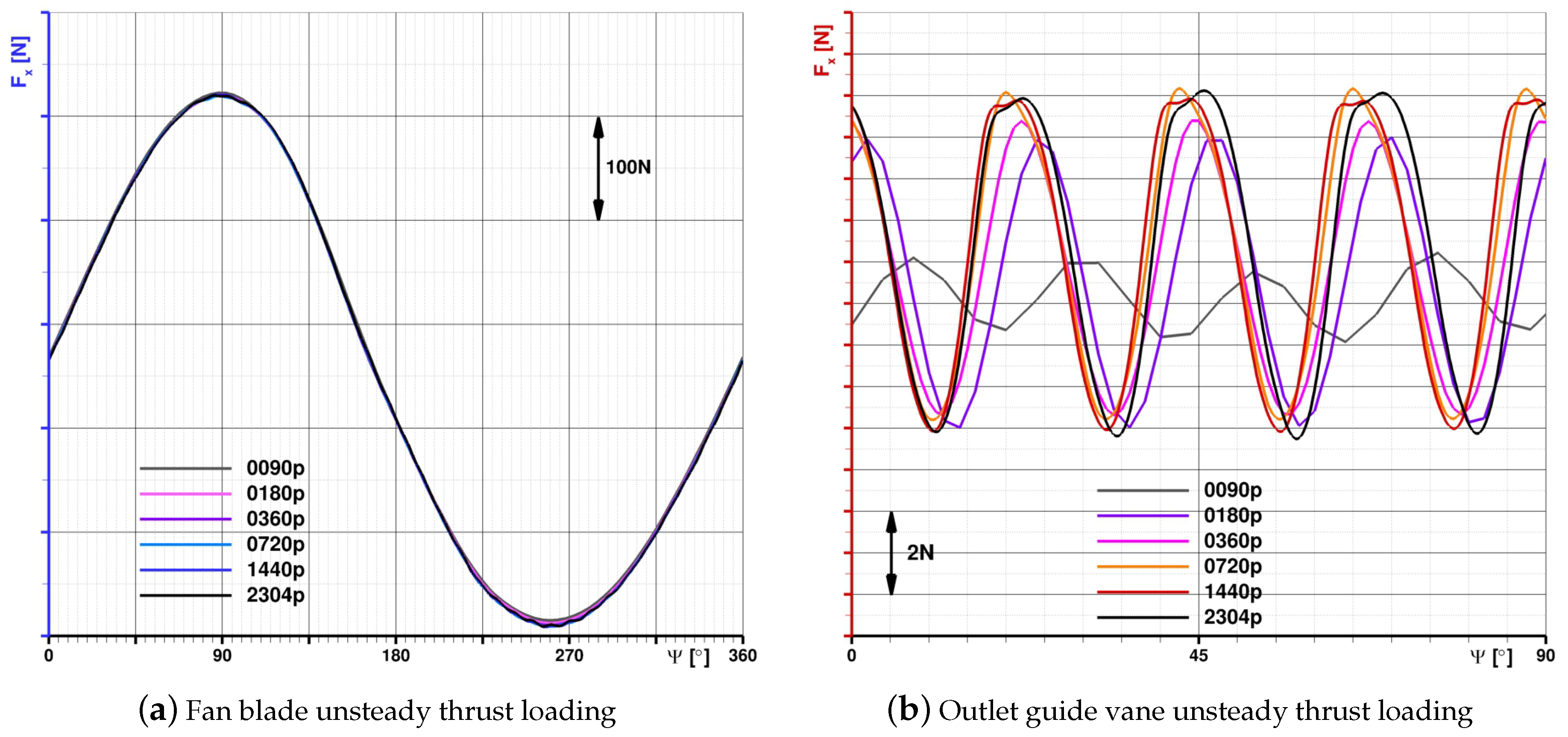
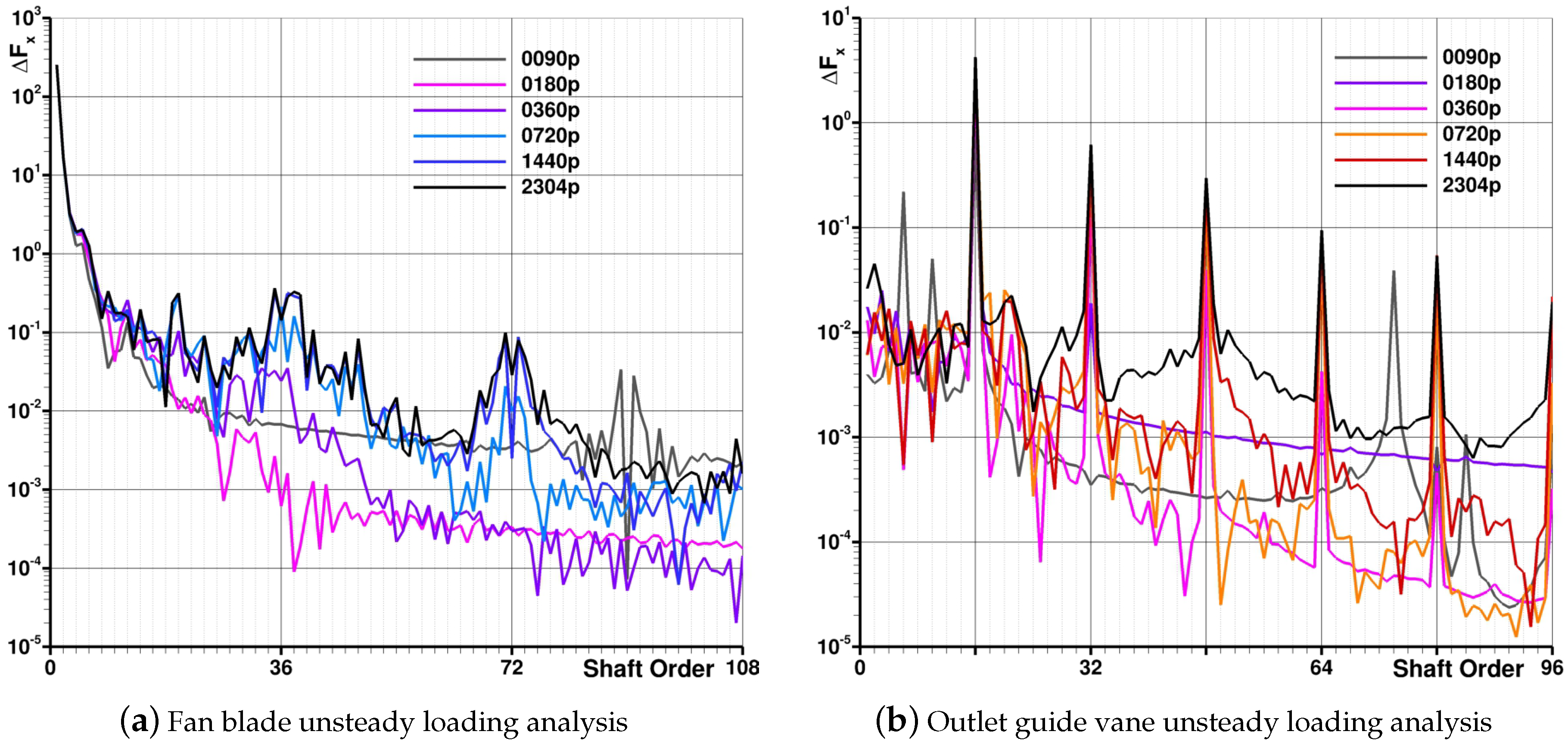
For the APP operating point, Figure 10 shows the time history of the unsteady axial loading development for a reference fan blade and the top outlet guide vane during one full rotor revolution. Figure 10a plots the results of the time step study on the highest density mesh for a reference fan blade during one full revolution. A similar analysis is shown in Figure 10b for a reference outlet guide vane, which, due to the 16-bladed fan, is affected by four fan blade passages during the plotted quarter rotation of the rotor. For the fan, at all temporal resolutions, the once per revolution sinusoidal oscillation of the blade loading due to the angle of attack of the engine is predicted equally well. However, the upstream potential flow impact of the OGV vanes on a fan blade is only well resolved when the time step is sufficiently small. This is evident when looking at the spectral analysis of the fan blade loading development in Figure 11a. The fundamental interaction occurring at a shaft order of 36 is only beginning to be captured well enough when at least 360 time steps per revolution are used. A convergence of the oscillation amplitudes, both at the fundamental interaction frequency and at higher harmonics thereof, is then evident as the time step is further refined. The unsteady loading of the outlet guide vane is driven fundamentally by the impingement of the fan blade wakes. As discussed above, the resolution of this flow feature is strongly dependent on the time-step size. Very evident already in the time history plotted in Figure 10b, the need for a temporal resolution of at least 720 time steps per rotor revolution to obtain a reasonable representation of the unsteady loads is more clearly highlighted by the spectral analysis shown in Figure 11b. Both images show that, as for the fan, the good match between the results at the two highest temporal resolution indicate a convergence in the capture of this unsteady loading is achieved.
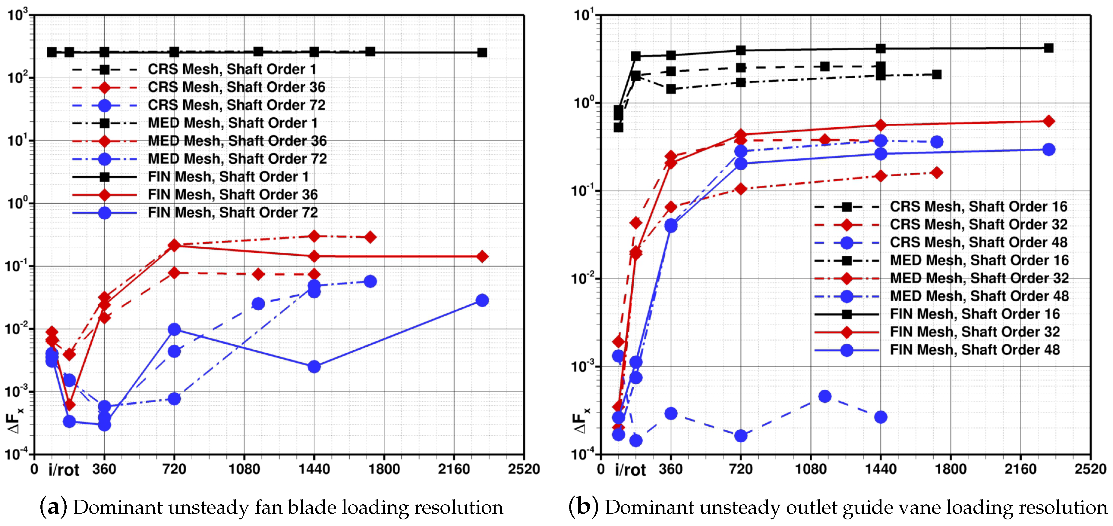
To substantiate the claim of an observed convergence of the unsteady loading amplitudes with higher temporal resolutions, the development of the amplitudes of the dominant unsteady loading for a fan blade at shaft orders 1, 36 and 72 is plotted in Figure 12a versus the number of time steps used to resolve one rotor revolution. The figure includes the results of the uRANS simulations across the various temporal resolutions for the coarse, medium and fine mesh densities.
The black lines, which show the amplitude predicted for the 1P-loading cycle for each mesh density and time step, reveal a negligible influence of both temporal and spatial resolution. For the interactions with the OGVs at shaft orders 36 and 72, however, a clear asymptotic trend is evident as the time step size is reduced. The unsteady loading at the fundamental interaction frequency (shaft order 32) shows that a good approximation of the loading amplitude is obtained for all meshes when at least 720 time steps are used for one fan rotation. For the coarse mesh, a result using 1440 time steps per revolution is also included. This is a temporal resolution that exceeds that for which the mesh was intended, as discussed in the chosen approach to the rotor–stator interface mesh and how it relates to the time step size choice. For the fundamental frequency, the graph shows that no change in amplitude prediction is found for this additional temporal resolution. Generally, it is seen that the amplitude predictions for the selected frequencies at a given temporal resolution show a small dependence on mesh density. At the fundamental interaction frequency, the coarse mesh leads to the lowest amplitudes being resolved, while medium and fine mesh results show very similar predictions as the temporal resolution is increased in each case. An analogous analysis of the unsteady loading amplitude predictions for an outlet guide vane in dependence of mesh density and temporal resolution is shown in Figure 12b. In this case, the predicted amplitudes at the fundamental interaction frequency (shaft order 16) and the higher harmonics thereof show values close to those at the highest temporal resolution being achieved when using 360 time steps per period. The exception is the result for the loading cycle occurring at shaft order 48 on the coarse mesh. Here, very low values are evident at all time step sizes, indicating that the spatial resolution is not sufficient on this mesh to properly account for this.
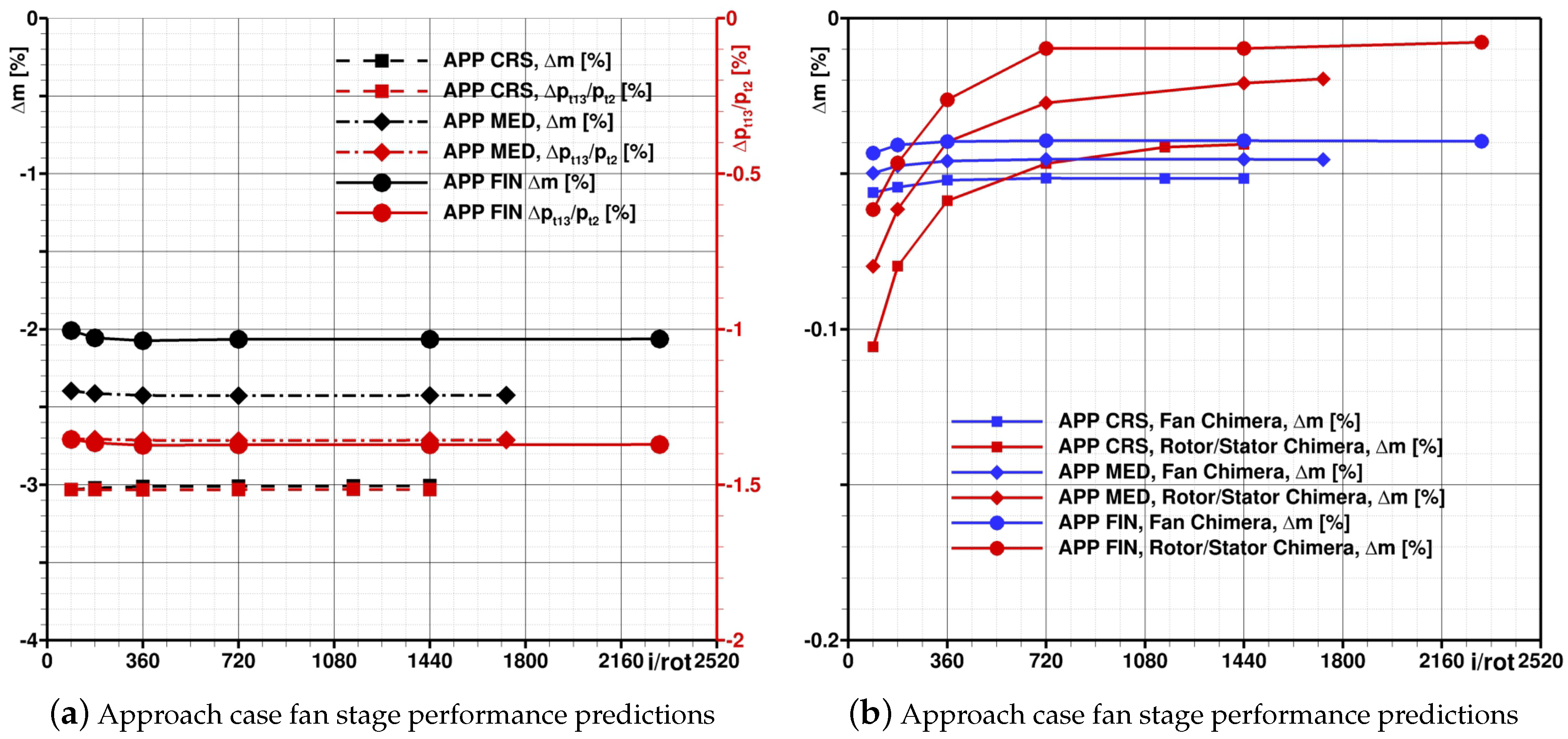
Figure 13a plots the mean uRANS fan stage performance predictions in terms of total mass flow and fan stage pressure ratios for the APP operating point. The mean fan performance metrics are the result of an averaging done for one full rotor revolution at the various temporal resolutions under study. For both metrics, the values are shown as deviations from the engine cycle model specifications and plotted versus the number of time steps used to resolve one full rotor revolution. The figure compares the coarse, medium and fine mesh results for the APP operating point. Both the mass flow rate and the fan stage pressure ratio are in reasonable agreement with the specifications, considering the challenging nature of this test case with a relatively low fan pressure ratio. The predicted fan face mass flow is within of the specifications on the coarse mesh and improves to matching the engine model data to within in on the fine mesh. The stage pressure ratio is in agreement with the reference data to within in all cases. A very small dependence of these mean performance metrics on the temporal resolution used in the uRANS simulations is seen, generally indicating that a temporal resolution of 360 time steps per rotor revolution is sufficient to obtain good mean performance predictions. The mesh density impact is more profound, showing an improved match with the specifications as the mesh is refined.
Figure 13b plots the discrepancy in air mass flow that is found across the Chimera interfaces—a potential concern due to the non-conservative nature of the overset mesh technique as implemented in TAU. However, the results show that the interpolation losses are very low at less than of the fan mass flow. These mass flow discrepancies are reduced both through mesh refinement and through improvements in temporal resolution. Of note is that the interpolation losses across the fan-OGV Chimera interface, which, as described above, was designed to feature co-incident nodes on both sides of boundary, shows the lowest values and a very strong asymptotic trend towards a value of 0 as the time step size is reduced. Thus, the non-conservative Chimera approach in TAU is found to not be an issue for the type of applications that DLR plans to be able to handle with the TAU Code using the simulation capabilities developed in the frame of ASPIRE.
Table 4 lists all the mean aerodynamic performance results achieved in the DLR TAU uRANS simulations. For all studied operating points, the results for the fan mass flow and the fan stage pressure ratio are listed as deviations from the Airbus specifications and in dependence of the grid density and selected time step sizes as available from the simulation results. While the challenging low fan pressure ratio APP case shows an offset of up to 3% versus the targets, the results for other operating points generally only show deviations on the order of about 1%. Both spatial and temporal resolutions have a small impact on the mean performance predictions, with the former being the more important consideration. For all cases, it can generally be stated that good quality predictions of mean performance metrics are possible using coarse time steps. For all cases, including the approach case as the main focus in this paper, the TAU predictions of the mean UHBR engine performance metrics are within the scatter of results found by the various partners in the ASPIRE project [26].
Table 5 lists the results of a grid convergence study for the fan performance metrics of the APP case. It is done using the approach proposed by the Fluids Engineering Division of the ASME [27,28], with refinements to the evaluation of the fine grid convergence index as proposed by Eca and Hoekstra [29,30]. The solution values listed for the fan mass flow and the fan pressure ratio are normalized with the corresponding values form the engine operating point specifications. For both performance metrics, a generally very good grid convergence can be accomplished. Larger values of the approximate relative fine grid error , the extrapolated relative fine grid error and the fine grid convergence index are consistently found for the mass flow. This performance metric may show larger errors due to the additional impact of the Chimera interpolation in addition to the spatial resolution of the global mesh refinement. However, in general, and for the fan pressure ration in particular, the errors are low and the extrapolated values are very close to the values of the fine and medium meshes. In line with the observations made based on Figure 13a, the medium and fine mesh simulations thus allow for good predictions of the mean aerodynamic performance of the engine.
4.2. Engine Boundary Condition Simulation and uRANS Results Comparison
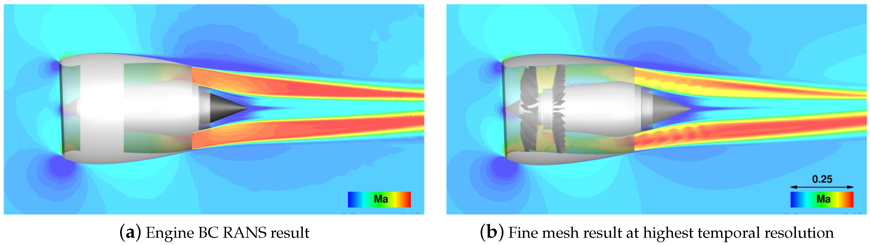
An initial qualitative comparison of the results achievable for the approach operating point case with both the uRANS and the engine BC approach is shown in Figure 14. The plots compare the mach number distribution on a plane through the engine centerline, showing the inlet flow, the external flow around the nacelle, and most importantly also the engine jet development. In general, a very favorable agreement between the uRANS result in Figure 14b and the engine BC result in Figure 14a is seen. A closer comparison of the jet development however shows that, while a perfectly axisymmetric jet is found for the engine boundary condition simulation, an asymmetry is seen in the uRANS results. Figure 14b shows higher Mach numbers in the bypass flow on the lower side of the engine than on the top. This is related to the angle of attack and the resulting non-uniform inflow to the fan. With the fully geometrically modeled fan and OGV an azimuthal variation in the blade and stator loading is the consequence, which also results in a non-axisymmetric jet development. The engine boundary condition by design neglects any correlation of flow non-uniformity seen by the fan to the engine exhaust boundary condition. The inlet also shows some very small differences relating to the fact that the uRANS simulation allows for a non-uniform mass flow distribution across the fan face that is not accounted for in the steady state RANS simulation with the engine boundary condition. At the lower lip, for example, where the fan loading is higher than at the top due to the angle of attack effect in the uRANS modeling, a slightly higher flow acceleration is seen than in the steady RANS analysis. While for most applications this is not a particular concern, there may be cases where the jet and inflow non-uniformity is important. Such cases could be studies of engine jet and wing or high-lift system interactions or also studies of configurations with a boundary layer ingesting integration of the engines. In particular, at the the low-speed flight conditions strong inflow perturbations occur, making a better understanding and modeling of the jet development—as well as a proper modeling of the non-uniform fan face flow—an important issue for external aerodynamics studies utilizing an engine modeling.
Table 6 compares the total engine mass flow rates found in the uRANS and the RANS simulations for the approach and sideline operating point cases. The values are normalized with the specified mass flow rates as computed by the engine cycle model. In general, both modeling approaches are relatively close with a deviation of less than for the total mass flow rate seen versus the engine model specifications. Thus, in terms of mean engine performance predictions, the boundary condition does deliver very good results, but, as stated, the neglect of non-axisymmetry in the physical flowfield may be an issue for some investigations.
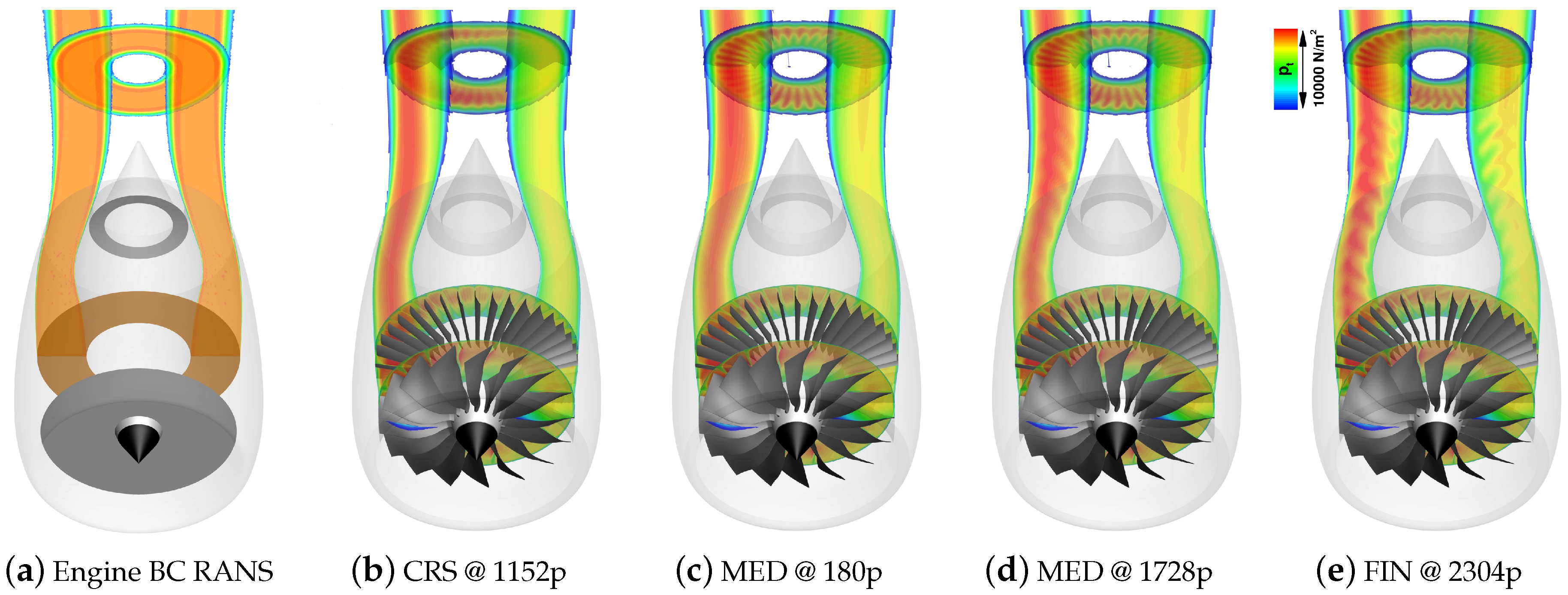
Figure 15 shows views of the UHBR engine from the front with total pressure contours added to highlight the engine jet development for the steady RANS simulation and the uRANS cases discussed in detail in the previous section. Here, the axisymmetry of jet that is inherent to the use of the engine boundary condition is clearly evident, with the total pressures essentially representing the mean azimuthal value found in the uRANS simulations. The coarse mesh result in Figure 15b shows that jet flow features relating to the interaction of blade wakes with the outlet guide vanes are not resolved sufficiently. For the medium mesh results shown in Figure 15c,d, it can be seen that the higher spatial resolution helps to enable the sustainment of the fan blade and outlet guide vane wakes as the temporal resolution is improved. As expected and plotted in Figure 15e, both the strong variations of the flow across the azimuth and the unsteady flow resulting from the wakes of the two blade rows are best captured in the uRANS simulations using the fine mesh.
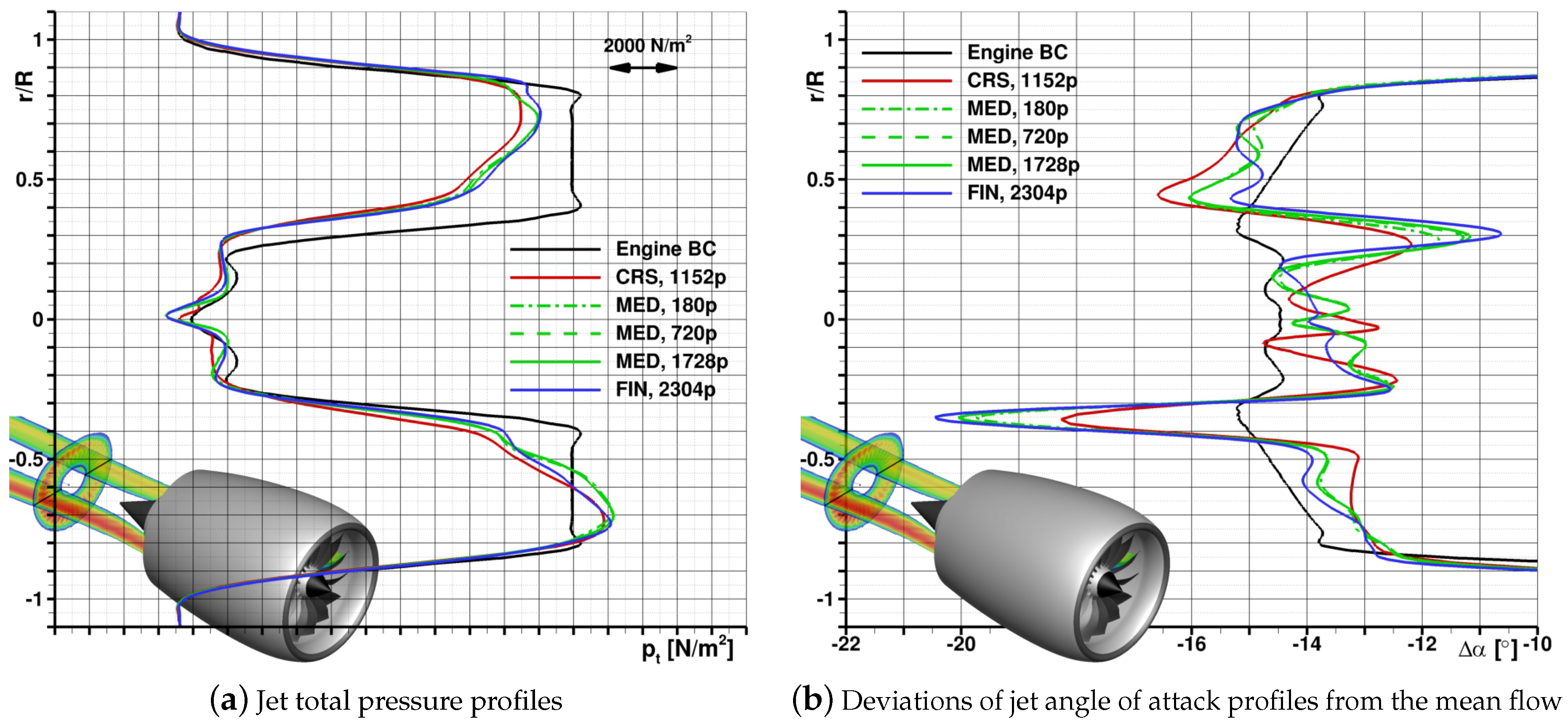
A quantitative evaluation of the jet characteristics at an axial position downstream of the nozzle that is representative for a position at which the flaps of an aircraft’s high lift system may be located is shown in Figure 16 and Figure 17. Figure 16 plots profiles of both the total pressure as well as the deviations of the angle of attack from the mean flow along rays in a horizontal plane through the engine centerline.
For the total pressure profiles in Figure 16a, all uRANS results are seen to be in very good agreement. This indicates that both mesh resolution and temporal resolution do not play a major role in capturing at least the mean flow characteristics in this case. The previously discussed discrepancy due to the uniform jet produced by the engine boundary condition model in the steady RANS result with the asymmetry seen in the uRANS results is the biggest difference to be observed. Furthermore, the combined effect of thicker boundary layers in the uRANS results as well as the unsteady nature of the bypass duct flow lead to a more pronounced mixing of the jet boundaries with the surrounding flow in the unsteady simulations. In the uRANS models, the boundary layers develop beginning at the nacelle lip and on the spinner, while in the RANS simulations boundary layer only start forming at the fan outlet boundary condition, they are thicker when they reach the nozzle in the former case. The steady RANS simulations also show a very constant total pressure profile across a large area of the bypass duct. This is again an inherent consequence of the models design, as constant total pressure and total temperatures are set on the entire plane representing the fan outlet. The variation of the loading distribution across the fan blade (and outlet guide vane) lead to a more non-uniform total pressure distribution across the bypass duct, which also reflect in the observable differences in the jet characteristics predicted by the two approaches. The angle of attack distribution in the jet as plotted in Figure 16b shows some larger differences between the various uRANS results. This relates mostly to the differing densities of the meshes, which allow the fine mesh results to sustain fan blade and outlet guide vane wakes to be sustained to this axial position, for example, leading to more pronounced peaks in the angles across the jet. The most important difference between the full geometric modeling of the fan and the boundary condition approach is again traceable to the lack of non-uniformity in the latter approach. These results thus do not capture the fact that larger angle of attack deviations are seen in the jet on the left side than on the right, which may be of importance for the high lift system of an aircraft with a very closely coupled under-wing mounting of these types of UHBR engines.
The jet characteristics for lines extending radially through the engine axis in the vertical plane at the same axial position are plotted in Figure 17. In general, the observations both for the total pressure as well as for the angle of attack deviations in the engine jet are comparable to the horizontal plane findings. The main difference is related to a slightly less pronounced asymmetry between the top and bottom half of the jet development than is found when comparing the left and right sides. Naturally, the presence of a wing and high lift system would lead to mutual interactions between the engine, the jet development and the interaction of the engine flowfield with the aircraft components. However, the general characteristics in terms of jet non-uniformity would certainly still apply, making the consideration of their impact at the aircraft level a worthwhile continuation of the present studies in the near future.
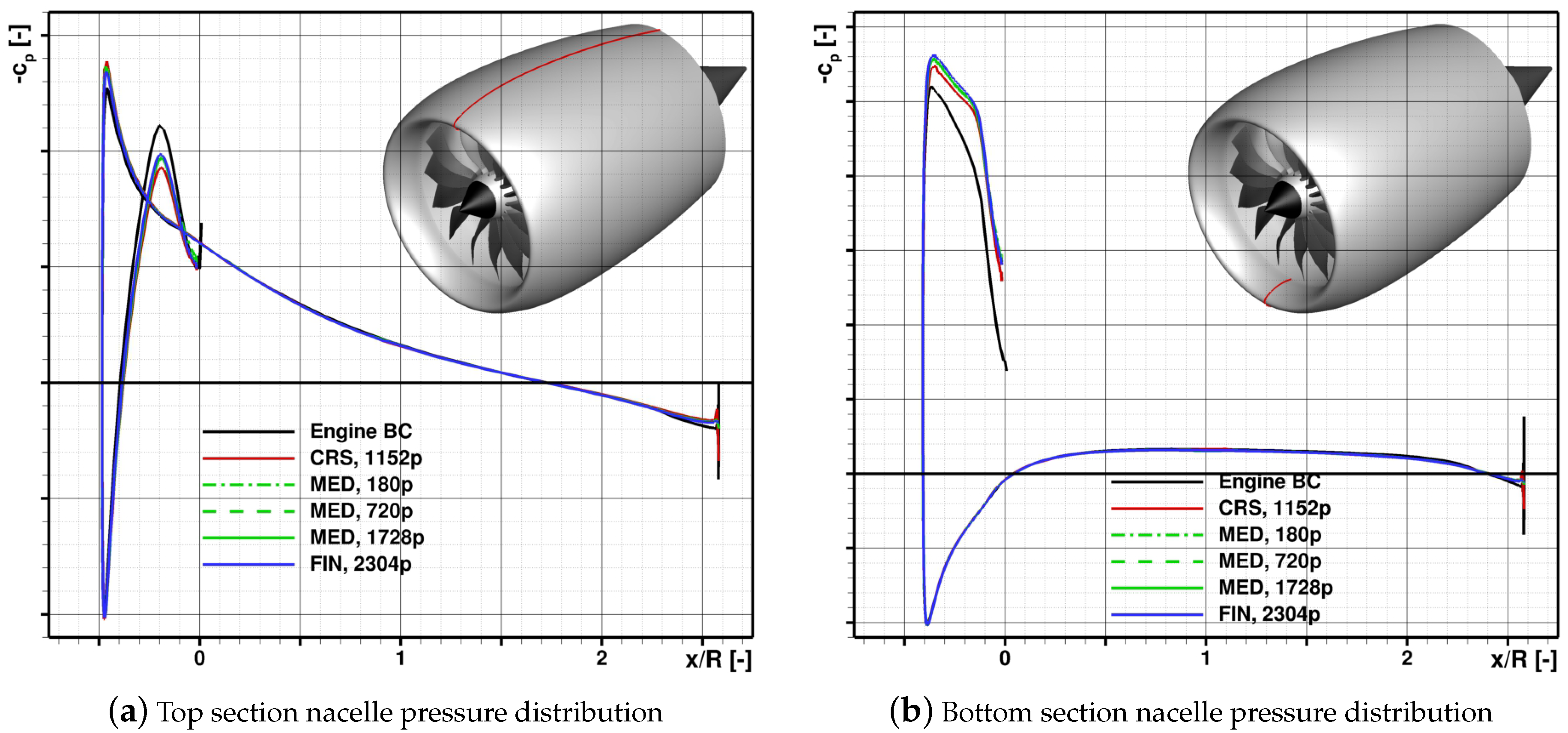
To understand the likely impact of the two fan modeling approaches compared in this article on some external aerodynamic aspects, Figure 18 plots a comparison of the nacelle pressure distributions drawn from all the previously discussed RANS and uRANS simulations. For most of the outer nacelle pressure distribution along the top and the bottom of the engine in Figure 18a,b, respectively, good agreement is seen between all of the uRANS as well as the steady RANS result using the engine boundary condition model. Stagnation points at the lip are also seen to be in good agreement for all cases, indicating that the external aerodynamics for this nacelle are well captured in all approaches. The main source of any differences, seen predominantly in the inlet as well as at the nacelle trailing edge, are again directly related to the capability of predicting the fan loading non-uniformity.
Looking at the trailing edge, it can be seen that for both the top section and the bottom section, the uRANS results—in good agreement amongst the different mesh densities and temporal resolutions presented—show a slightly different pressure than seen in the RANS result. The engine boundary condition approach leads to an azimuthally uniform jet in terms of all relevant flow properties, while there were notable differences in jet velocities for the uRANS modeling approach, as seen for example in Figure 14. Similarly, a more highly loaded fan at the bottom than at the top nacelle, properly represented when the fan stage is fully modeled in the uRANS approach, leads to a higher acceleration of the flow in the latter simulation results into the fan on the bottom lip. Subtle differences are visible between the uRANS results on the different meshes, with the highest suction peaks observed for the fine mesh case. Conversely, with a relatively low fan loading occurring at the top, the unsteady simulations show smaller suction peaks on the inner lip at the top of the nacelle.
For the external drag of the engine, as evaluated through a nacelle surface integration from the stagnation line on the inlet lip to the trailing edge at the bypass duct nozzle, the variation in the suction peaks visible at the top of the nacelle in Figure 18a leads to notable differences when comparing the various results. In line with the observed trends on the suction peaks, where lower pressures lead to negative drag values due to the curvature of the lip, the uRANS results show that lower pressure drag values for the nacelle results, with the coarse mesh nacelle drag lowest at of the RANS approach value, while those of the medium and the fine mesh increase to values of and , respectively. While an increase in pressure drag can thus be observed as the mesh is refined in the uRANS analysis, the trend in viscous drag is the inverse. This reduction in viscous drag at higher spatial resolution is most likely directly linked to the reduced flow acceleration on the nacelle upper lip. Thus, total drag for the nacelle in the uRANS studies is , and for the coarse, medium and fine grid cases, respectively—indicating that non-uniform fan inflow effects for more highly integrated engine–airframe configurations can be an important consideration in the thrust–drag bookkeeping at the aircraft level.
5. Conclusions
To identify benefits, short-comings and costs of various engine modeling approaches in external aerodynamics focused CFD simulations of modern engine–airframe configurations with the DLR TAU-Code, the DLR Institute of Aerodynamics and Flow Technology is comparing a high-fidelity uRANS fan-stage simulation with a classical engine boundary condition RANS approach. For the uRANS simulations, a successfully established process chain used for previous CROR studies is adapted to the present UHBR turbofan simulations and a detailed numerical study, addressing both spatial and temporal resolution aspects, was performed.
It was found that mean performance predictions for metrics such as overall fan face mass flow and fan stage pressure ratios, the simulation results show a good agreement with the engine model specifications even when using relatively coarse time steps. While for the CROR studies, mesh density was found to have a negligible impact on the quality of the mean performance predictions, the present results indicate that the coarse meshes used in this study lead to notably larger deviations from the specifications than seen on the medium and fine grids. Furthermore, it was shown that the non-conservative Chimera approach in TAU does not lead to significant air mass flow issues, with a careful consideration of spatial and temporal resolutions allowing a reduction of interpolation losses to near-zero levels.
Investigations of engine jet as well as inlet and external nacelle aerodynamic characteristics also showed only a negligible impact of temporal resolution on the prediction of relevant flow phenomena. An adequate resolution of the unsteady fan blade and outlet guide vane forces on the other hand does require a sufficiently small physical time step to properly capture the relevant and underlying aerodynamic phenomena, i.e., the interaction of the fan blade wakes with the outlet guide vanes. This will be an important consideration for aeroacoustic investigations, which often draw on uRANS results, or perhaps for some aspects relating to fan blade and outlet guide vane structural design and aeroelasticity.
While uRANS simulations are today still a very expensive numerical approach for many application, there may be justification for employing coarse to medium mesh studies for relevant complex engine–airframe installations using relatively large time steps, as they do yield quality aerodynamic data not easily obtained by other means and may also deliver data of direct use for fan blade structural design and aeroelasticity. The classic engine boundary condition, in use for decades to model engine flow fields in steady RANS studies, proves to deliver good mean engine performance predictions. However, for cases such as the short inlet UHBR engine studied here, the inherent lack of azimuthally non-uniform flow characteristics in this modeling approach may make it a poor choice for some foreseen engine–airframe analyses. Currently, work on adapting and applying an actuator disc model available in TAU is being done. Both this approach and a body force model, which is also being implemented in the code, are expected to yield an intermediate complexity/effort numerical approach, to enable a good quality representation of non-uniform in- and outflow effects for the engine at a low computational cost.
Funding
This research received funding in the frame of the Clean Sky 2 Joint Undertaking under the European Union Horizon 2020 research and innovation program, grant agreement No. 681856–ASPIRE.
Acknowledgments
The author gratefully acknowledges the support of the ASPIRE consortium partners for enabling the publication of this paper as well as for a very fruitful collaboration in the project.
Conflicts of Interest
The author declares no conflict of interest.
Abbreviations
| ADP | Aerodynamic design engine operating point |
| APP | Approach engine operating point |
| BC | Boundary Condition |
| BSN | Buzz Saw Noise engine operating point |
| CFD | Computational Fluid Dynamics |
| CROR | Contra-Rotating Open Rotor |
| CRS | Coarse mesh |
| CS2 | EU Clean Sky 2 Research Project |
| CUT | Cutback engine operating point |
| DLR | German Aerospace Center |
| FIN | Fine mesh |
| MED | Medium (density) mesh |
| OGV | Outlet Guide Vane |
| RANS | Reynolds Averaged Navier–Stokes |
| SID | Sideline engine operating point |
| UHBR | Ultra High Bypass Ratio |
| uRANS | Unsteady Reynolds Averaged Navier–Stokes |
| Angle of attack | |
| Blade azimuthal position | |
| Density, [kg/m] | |
| Solution value on the fine, medium or coarse grid | |
| Extrapolated solution value | |
| Pressure coefficient, , [-] | |
| Approximate relative fine grid error | |
| Extrapolated relative fine grid error | |
| h | Altitude, [ft] |
| Forces in the cartesian coordinate system, [N] | |
| Fine grid convergence index | |
| m | Mass flow rate, [kg/s] |
| Mach number, [-] | |
| Fan rotational speed, [rpm] | |
| p | Pressure, [N/m] |
| Total pressure, [N/m] | |
| Reference pressure, [N/m] | |
| q | Dynamic pressure, , [N/m] |
| r | Radial position, [m] |
| Fine to medium grid ratio, [-] | |
| Medium to coarse grid ratio, [-] | |
| R | Fan reference radius, [m] |
| Free stream velocity, [m/s] | |
| Cartesian coordinate system positions, [m] |
References
- Stuermer, A. Assessing Turbofan Modeling Approaches in the DLR TAU-Code for Aircraft Aerodynamics Investigations. In Proceedings of the AIAA SciTech 2019, San Diego, CA, USA, 7–11 January 2019. Number AIAA 2019-0277. [Google Scholar]
- Laban, M.; Kok, J.; Brouwer, H. CFD/CAA Analysis of UHBR Engine Tonal Noise. In Proceedings of the AIAA Aviation 2018, Atlanta, GA, USA, 25–29 June 2018. Number AIAA 2018-3780. [Google Scholar]
- Burlot, A.; Sartor, F.; Vergez, M.; Meheut, M.; Barrier, R. Method Comparison for Fan Performance in Short Intake Nacelle. In Proceedings of the AIAA Aviation 2018, Atlanta, GA, USA, 25–29 June 2018. Number AIAA 2018-4204. [Google Scholar]
- Peters, A.; Spakovszky, Z.S.; Lord, W.K.; Rose, B. Ultrashort Nacelles for Low Fan Pressure Ratio Propulsors. J. Turbomach. 2014, 137, 021001. [Google Scholar] [CrossRef] [Green Version]
- Thollet, W.; Dufour, G.; Carbonneau, X.; Blanc, F. Body-force modeling for aerodynamic analysis of air intake—Fan interactions. Int. J. Numer. Methods Heat Fluid Flow 2016, 26, 2048–2065. [Google Scholar] [CrossRef]
- Akaydin, H.D.; Pandya, S.A. Implementation of a Body Force Model in OVERFLOW for Propulsor Simulations. In Proceedings of the 35th AIAA Applied Aerodynamics Conference, Denver, CO, USA, 5–9 June 2017. [Google Scholar] [CrossRef]
- Hall, D.K.; Greitzer, E.M.; Tan, C.S. Analysis of Fan Stage Conceptual Design Attributes for Boundary Layer Ingestion. J. Turbomach. 2017, 139, 071012. [Google Scholar] [CrossRef] [Green Version]
- Schnell, R.; Goldhahn, E.; Julian, M. Design and Performance of a Low Fan-Pressure-Ratio Propulsion System. In Proceedings of the 25th International Symposium on Air Breathing Engines ISABE 2019, Canberra, Australia, 22–27 September 2019. Number ISABE-2019-24017. [Google Scholar]
- Stuermer, A. Unsteady CFD Simulations of Contra- Rotating Propeller Propulsion Systems. In Proceedings of the 44th AIAA/ASME/SAE/ASEE Joint Propulsion Conference, Hartford, CT, USA, 21–28 July 2008. Number AIAA 2008-5218. [Google Scholar]
- Stuermer, A.; Yin, J. Low-Speed Aerodynamics and Aeroacoustics of CROR Propulsion Systems. In Proceedings of the 15th AIAA/CEAS Aeroacoustics Conference, Miami, FL, USA, 11–13 May 2009. Number AIAA 2009-3134. [Google Scholar]
- Stuermer, A.; Yin, J. Installation impact on pusher CROR engine low speed performance and noise emission characteristics. Int. J. Eng. Syst. Model. Simul. 2012, 4, 59–68. [Google Scholar] [CrossRef]
- Stuermer, A.; Akkermans, R. Validation of Aerodynamic and Aeroacoustic Simulations of Contra-Rotating Open Rotors at Low-Speed Flight Conditions. In Proceedings of the AIAA Aviation 2014, Atlanta, GA, USA, 16–20 June 2014. Number AIAA 2014-3133. [Google Scholar]
- Stuermer, A. Validation of Installation Effect Predictions Through Simulations of CRORs at Low-Speed Flight Conditions. In Proceedings of the AIAA Aviation 2015, Atlanta, GA, USA, 22–26 June 2015. Number AIAA 2015-2886. [Google Scholar]
- Stuermer, A.W. Validation of uRANS-Simulations of Contra-Rotating Open Rotor-Powered Aircraft at Take-Off Conditions. In Proceedings of the 2018 AIAA Aerospace Sciences Meeting, Kissimmee, FL, USA, 8–12 January 2018. [Google Scholar] [CrossRef]
- Gerhold, T. Overview of the Hybrid Rans Code TAU; Springer: Berlin/Heidelberg, Germany, 2005; Volume 89, pp. 81–92. [Google Scholar]
- Jameson, A.; Schmidt, W.; Turkel, E. Numerical Solution of the Euler Equations by Finite Volume Methods Using Runge-Kutta Time Stepping Schemes. In Proceedings of the 14th AIAA Fluid and Plasma Dynamic Conference, Palo Alto, CA, USA, 23–25 June 1981. Number AIAA 81-1259. [Google Scholar]
- Spalart, P.; Allmaras, S. A One-Equation Turbulence Model for Aerodynamic Flows. In Proceedings of the 30th Aerospace Sciences Meeting and Exhibit, Reno, NV, USA, 6–9 January 1992. Number AIAA 92-0439. [Google Scholar]
- Allmaras, S.; Johnson, F.; Spalart, P. Modifications and clarifications for the implementation of the Spalart-Allmaras turbulence model. In Proceedings of the Seventh International Conference on Computational Fluid Dynamics (ICCFD7), Big Island, HI, USA, 9–13 July 2012; pp. 1–11. [Google Scholar]
- Jameson, A. Time Dependent Calculations Using Multigrid, with Applications to Unsteady Flows Past Airfoils and Wings. In Proceedings of the 10th Computational Fluid Dynamics Conference, Honolulu, HI, USA, 24–26 June 1991. [Google Scholar]
- Langer, S.; Schwöppe, A.; Kroll, N. The DLR Flow Solver TAU—Status and Recent Algorithmic Developments. In Proceedings of the 52nd Aerospace Sciences Meeting, National Harbor, MD, USA, 13–17 January 2014. [Google Scholar]
- Langer, S.; Schwöppe, A.; Kroll, N. Investigation and Comparison of Implicit Smoothers Applied in Agglomeration Multigrid. AIAA J. 2015, 53, 2080–2096. [Google Scholar] [CrossRef]
- Madrane, A.; Heinrich, R.; Gerhold, T. Implementation of the Chimera Method in the Unstructured Hybrid DLR Finite Volume TAU-Code. In Proceedings of the 6th Overset Composite Grid and Solution Technology Symposium, Ft. Walton Beach, FL, USA, 8–10 October 2002; pp. 524–534. [Google Scholar]
- Madrane, A.; Raichle, A.; Stuermer, A. Parallel Implementation of a Dynamic Unstructured Chimera Method in the DLR Finite Volume TAU-Code. In Proceedings of the 12th Annual Conference of the CFD Society of Canada, Ottawa, ON, Canada, 9–11 May 2004; pp. 524–534. [Google Scholar]
- Schwarz, T. Ein Blockstrukturiertes Verfahren zur Simulation der Umströmung Komplexer Konfigurationen; Technical Report; TU Braunschweig: Braunschweig, Germany, 2005. [Google Scholar]
- Raichle, A. Extension of the Unstructured TAU-Code for Rotating Flows. In Proceedings of the DGLR-STAB Symposium, Bremen, Germany, 16–18 November 2004. [Google Scholar]
- Meheut, M.; Sartor, F.; Vergez, M.; Laban, M.; Schnell, R.; Stuermer, A.; Lefevre, G. Assessment of Fan/Airframe aerodynamic performance using 360∘ uRANS computations: Code-to-Code comparison between ONERA, DLR, NLR and Airbus. In Proceedings of the AIAA SciTech 2019, San Diego, CA, USA, 7–11 January 2019. Number AIAA 2018-0582. [Google Scholar]
- Roache, P. Perspective: A method for uniform reporting of grid refinement studies. J. Fluids Eng. 1994, 116, 405–413. [Google Scholar] [CrossRef]
- Celik, I.B.; Ghia, U.; Roache, P.J.; Freitas, C.J. Procedure for Estimation and Reporting of Uncertainty Due to Discretization in CFD Applications. J. Fluids Eng. 2008, 130, 078001. [Google Scholar] [CrossRef] [Green Version]
- Eça, L.; Hoekstra, M. Evaluation of numerical error estimation based on grid refinement studies with the method of the manufactured solutions. Comput. Fluids 2009, 38, 1580–1591. [Google Scholar] [CrossRef]
- Rumsey, C.L.; Carlson, J.; Ahmad, N. FUN3D Juncture Flow Computations Compared with Experimental Data. In Proceedings of the AIAA SciTech 2019, San Diego, CA, USA, 7–11 January 2019. [Google Scholar] [CrossRef]
Figure 1.
Challenging engine–airframe integration scenarios with significant mutual aerodynamic interactions between the airframe and the engines fan stage.
Figure 1.
Challenging engine–airframe integration scenarios with significant mutual aerodynamic interactions between the airframe and the engines fan stage.

Figure 2.
ASPIRE isolated UHBR turbofan (geometry not to scale).

Figure 3.
CFD modeling of the isolated ASPIRE UHBR turbofan in the present study.

Figure 4.
Mesh setup for the isolated UHBR uRANS simulations.

Figure 5.
Engine station definitions (geometry not to scale).

Figure 6.
Non-axisymmetric fan inflow due to the very short intake and high angle of attack.

Figure 7.
Fine mesh result for the isolated UHBR engine at the approach operating point.

Figure 8.
Total pressure contours showing the impact of the time step size on fan blade wake resolution and sustainment (APP case medium mesh results, geometries not to scale).
Figure 8.
Total pressure contours showing the impact of the time step size on fan blade wake resolution and sustainment (APP case medium mesh results, geometries not to scale).

Figure 9.
Axial development of fan blade wake total pressure profiles at a radial position of r/R = 0.79 for the APP operating point.
Figure 9.
Axial development of fan blade wake total pressure profiles at a radial position of r/R = 0.79 for the APP operating point.

Figure 10.
Temporal resolution impact on fan and OGV blade unsteady axial loading (APP case fine mesh).
Figure 10.
Temporal resolution impact on fan and OGV blade unsteady axial loading (APP case fine mesh).

Figure 11.
Spectral analysis of fan and OGV blade unsteady axial loading (APP case fine mesh).

Figure 12.
Development of unsteady loading predictions with temporal and spatial resolution for a fan and OGV blade (APP case).
Figure 12.
Development of unsteady loading predictions with temporal and spatial resolution for a fan and OGV blade (APP case).

Figure 13.
Spatial and temporal resolution impact on mean fan performance and mass flow predictions.
Figure 13.
Spatial and temporal resolution impact on mean fan performance and mass flow predictions.

Figure 14.
Engine centerline Mach number contours (APP case, geometries not to scale).

Figure 15.
Total pressure contours showing RANS/uRANS modeling of UHBR jet characteristics.

Figure 16.
Jet characteristics in the horizontal plane one fan diameter downstream of the nozzle.

Figure 17.
Jet characteristics in the vertical plane one fan diameter downstream of the nozzle.

Figure 18.
Comparison of CFD modeling influence on nacelle pressure distributions for the APP case.


Table 1.
Currently studied UHBR engine operating points.
| Altitude h [ft] | Flight Speed Ma [-] | Incidence Angle α [°] | Fan Rotation Speed N1/N1,ADP [%] | |
|---|---|---|---|---|
| SID: Take-Off Sideline | 700 | 0.27 | 15 | 110 |
| BSN: Take-Off Buzz-Saw Noise | 700 | 0.27 | 15 | 120 |
| CUT: Take-Off Cutback | 2200 | 0.27 | 15 | 96 |
| APP: Approach | 400 | 0.23 | 10 | 64 |
Table 2.
Isolated UHBR engine mesh family overview.
| Coarse Mesh | Medium Mesh | Fine Mesh | |
|---|---|---|---|
| Farfield | |||
| Nacelle | |||
| Fan | |||
| OGV | |||
| Total |
Table 3.
Computational matrix of investigated temporal resolutions, listed as time steps per rotor revolution.
Table 3.
Computational matrix of investigated temporal resolutions, listed as time steps per rotor revolution.
| Fine Mesh | Medium Mesh | Coarse Mesh |
|---|---|---|
| 90 | 90 | 90 |
| 180 | 180 | 180 |
| 360 | 360 | 360 |
| 720 | 720 | 720 |
| 1440 | 1440 | 1152 |
| 2304 | 1728 | - |
Table 4.
Aerodynamic fan performance predictions as deviations from the Airbus specifications for mass flow and fan pressure ratio.
Table 4.
Aerodynamic fan performance predictions as deviations from the Airbus specifications for mass flow and fan pressure ratio.
| Coarse Mesh | Medium Mesh | Fine Mesh | ||||
|---|---|---|---|---|---|---|
| APP | 1152 | 0180 | 1728 | 0180 | 2304 | 0180 |
| Fan Mass flow | ||||||
| Fan Pressure Ratio | ||||||
| SID | 1152 | 0180 | 1728 | 0180 | 0720 | 0180 |
| Fan Mass flow | ||||||
| Fan Pressure Ratio | ||||||
| BSN | 1152 | - | - | |||
| Fan Mass flow | - | - | ||||
| Fan Pressure Ratio | - | - | ||||
| CUT | 1152 | - | - | |||
| Fan Mass flow | - | - | ||||
| Fan Pressure Ratio | - | - | ||||
Table 5.
Grid convergence study results for the fan performance metrics.
| Normalized Fan Mass Flow | Normalized Fan Pressure Ratio | |
|---|---|---|
| Grid ratio | ||
| Grid ratio | ||
| Fine grid value | ||
| Medium grid value | ||
| Coarse grid value | ||
| Extrapolated value | ||
| Approximate relative fine grid error | ||
| Extrapolated relative fine grid error | ||
| Fine grid convergence index |
Table 6.
Comparison of uRANS and RANS predictions of fan face mass flow rates at the APP and SID operating point, normalized to the engine model specifications.
Table 6.
Comparison of uRANS and RANS predictions of fan face mass flow rates at the APP and SID operating point, normalized to the engine model specifications.
| APP | SID | |
|---|---|---|
| uRANS | 0.9799 | 1.0186 |
| RANS | 0.9840 | 1.0096 |
© 2019 by the author. Licensee MDPI, Basel, Switzerland. This article is an open access article distributed under the terms and conditions of the Creative Commons Attribution (CC BY) license (http://creativecommons.org/licenses/by/4.0/).
Share and Cite
MDPI and ACS Style
Stuermer, A. DLR TAU-Code uRANS Turbofan Modeling for Aircraft Aerodynamics Investigations. Aerospace 2019, 6, 121. https://0-doi-org.brum.beds.ac.uk/10.3390/aerospace6110121
AMA Style
Stuermer A. DLR TAU-Code uRANS Turbofan Modeling for Aircraft Aerodynamics Investigations. Aerospace. 2019; 6(11):121. https://0-doi-org.brum.beds.ac.uk/10.3390/aerospace6110121
Chicago/Turabian StyleStuermer, Arne. 2019. "DLR TAU-Code uRANS Turbofan Modeling for Aircraft Aerodynamics Investigations" Aerospace 6, no. 11: 121. https://0-doi-org.brum.beds.ac.uk/10.3390/aerospace6110121
Note that from the first issue of 2016, this journal uses article numbers instead of page numbers. See further details here.