Article

LEO Object’s Light-Curve Acquisition System and Their Inversion for Attitude Reconstruction

1
Department of Mechanical and Aerospace Engineering (DIMA), University of Rome “La Sapienza”, 00184 Rome, Italy
2
Institute of Complex System (ICS), National Council of Research (CNR), UOS Sapienza, 00185 Rome, Italy
3
Department of Astronautics, Electric and Energy Engineering (DIAEE), University of Rome “La Sapienza”, 00184 Rome, Italy
*
Author to whom correspondence should be addressed.
Submission received: 13 November 2020 / Revised: 4 December 2020 / Accepted: 8 December 2020 / Published: 23 December 2020
(This article belongs to the Special Issue Orbit Determination of Earth Orbiting Objects)

Abstract

:
In recent years, the increase in space activities has brought the space debris issue to the top of the list of all space agencies. The fact of there being uncontrolled objects is a problem both for the operational satellites in orbit (avoiding collisions) and for the safety of people on the ground (re-entry objects). Optical systems provide valuable assistance in identifying and monitoring such objects. The Sapienza Space System and Space Surveillance (S5Lab) has been working in this field for years, being able to take advantage of a network of telescopes spread over different continents. This article is focused on the re-entry phase of the object; indeed, the knowledge of the state of the object, in terms of position, velocity, and attitude during the descent, is crucial in order to predict as accurately as possible the impact point on the ground. A procedure to retrieve the light curves of orbiting objects by means of optical data will be shown and a method to obtain the attitude determination from their inversion based on a stochastic optimization (genetic algorithm) will be proposed.

1. Introduction

The increase in artifacts placed in orbit every year exponentially affects the amount of space debris surrounding the Earth. The European Space Agency (ESA) has estimated that currently, there are about 750,000 orbiting debris larger than 1 cm [1]; this situation worries both the space agencies of any country and the private industry operating in the aerospace sectors because of possible collisions in flight between their systems and a debris swarm [2,3]. Current technology does not allow the removal of uncontrolled debris from orbit but only its monitoring and over the years; a large amount monitoring systems have been developed, which made it possible to track and catalog about 23,000 uncontrolled object [1].
Nowadays, the most comprehensive and available catalog of uncontrolled objects is the North American Aerospace Defense Command (NORAD) one. The American institution periodically releases orbital information about the objects in the form of Two Line Elements (TLE), which report, ordered in two strings of code, both a set of Kozai–Brouwer mean orbital elements and a term, BSTAR (B∗), referring to the area over mass ratio [4]. Unfortunately, the TLEs cannot be used in Space Surveillance and Tracking (SST) as they characterize the orbital motion of tracked object in a purely theoretical model, which accumulate, during each single orbit, the sum of all the variables not considered by the ideal model [5]. For this reason, after a certain period, the errors accumulated by the TLE become so large that they no longer describe the orbit of the tracked object, involving such a level of inaccuracy that it is necessary to update them through a new series of direct measurements and a consequent release of new TLEs after a few hours [6,7].
Due to the huge number of probabilistic variables that contribute to changing the orbit of an object, any predictive model developed will never describe the rigorous behavior of the object. Today, the research is oriented towards continuous and frequent direct measurements of debris which make it possible both to know the position of the object with very low margins of error and to contribute to the development of innovative techniques aimed at improving existing mathematical models. The knowledge of the state of the object is fundamental to understand the behavior of the object itself, therefore it must be observed. Many observation systems are used for the observation of debris and their direct measurement: laser, radar and optical systems.
In this paper, a set of innovative techniques will be discussed, which, by exploiting direct optical observations, make it possible to derive the flight attitude of uncontrolled object.
In particular, a methodology will be discussed which makes it possible to obtain the “light curves” from direct optical observations of debris, acquired from different observatories at same time (simultaneous multi-site observation) and it will be discussed how, through their inversion, it will be possible to derive their attitude dynamics. The knowledge of the attitude dynamics makes it possible to significantly improve the terms related to the atmospheric drag responsible for the orbital degradation of any orbiting object and, consequently, the predictive models can also be improved. Furthermore, performing simultaneous multi-site observation drastically reduces the error of the flight level altitude and makes it possible to attribute very precisely the term related to the effect of atmospheric drag at the observed debris.
In recent years, the Sapienza Space System and Space Surveillance (S5Lab) gained experience in satellite systems manufacturing and launches, and in the space debris field [8,9,10,11,12,13,14,15,16,17,18], operating networks [19,20,21,22,23,24,25] of completely remote optical observatories, which are able to observe, catalogue and identify a huge number of objects both known that unknown, thanks to which it was possible to refine the correlation between light curves and attitude dynamics of the observed debris. For these reasons, every methodology discussed in this paper is strongly based on a great number of observations, which makes it possible to obtain reliable and solid results.

2. System Description

The S5Lab observatories network includes many telescopes located in different countries around the world [19]. To obtain the real light-curve presented in this article, the Remote Space Debris Observation System (RESDOS) and the Sapienza Coupled University Debris Observatory (SCUDO) observatories, located in Rome (RM) and Collepardo (FR), respectively, are used. In both systems, a scientific Complementary Metal-Oxide Semiconductor (sCMOS) sensor is installed integrally with the main telescope and its mount, so the systems are able to track the satellite and acquire the video in real time. The sCMOS sensor makes it possible to obtain a readout rate higher than Charge Coupled Device (CCD) sensor, ensuring a large value of frame rate (fps). Moreover, the mounts used to move the telescope are able to track every satellite in every orbital regime Low Earth Orbit (LEO), Medium Earth Orbit (MEO), and Geostationary Earth Orbit (GEO). Both systems are equipped with the same sCMOS sensor and mount and in the Table 1 a summary of the main characteristics of the two systems is indicated.
The simultaneous multi-site observations require an extremely precise acquisition synchronization of the order of the milliseconds or tighter. The synchronization error must be as small as possible in order to obtain a better integration of the data acquired from the two observatories. Once the object’s enter into the range of visibility, the sCMOS sensor receives a trigger signal for starting the recording. To avoid synchronization errors, a GPS receiver is installed in both systems. The Pulse Per Second (PPS) of the GPS signal and the camera’s Lag Time, i.e., the time between the shutter release (trigger signal) and the actual shoot, are taken into account: the first one is negligible [26], whereas the latter is constant (for the described system) and therefore can be correct.

3. Photometric Routine

The real light-curve of the object is the variation over time of its apparent magnitude. This magnitude is calculated with respect to the stars present in the field of view in each frame. The stars’ catalog magnitude is obtained from the star field resolution, and this is performed by a local version of Astrometry.net software (version 0.84, Dustin Lang, Waterloo, Canada) [27]. For each frame, celestial coordinates, pixel coordinates and bolometric (B) and visual (V) catalogue magnitudes for each star are known. The star catalogue used to solve the star field is the Tycho-2 [28].

3.1. Reference Star Selection Criterion

Many stars may be present in the field of view, but not all of them can be used as a reference for calculating the magnitude of the object. Moreover, to calculate the apparent magnitude of one star with respect to another, the two stars must be approximately of the same spectral class, that is, be of the same color. The color of the star can be determined from its temperature, and the temperature can be obtained through the knowledge of the difference between bolometric and visual magnitude (B–V), as described in [29]. It has been assumed that if B–V < 0.3 then the star is blue, otherwise red, since for B–V = 0.3 a star temperature of about 7000 K is obtained, which corresponds approximately to a white star [29]. In addition, the stars that are at the edges of the field of view are excluded. Before proceeding with the calculation of the intensity of the star, it is necessary to calibrate the image in order to correct phenomena due to the sensor such as the variation in quantum efficiency, vignetting, dark current, bias level and the gain for AD conversion. The applied method is known as standard calibration [30]. To calculate the apparent magnitude of a star it is necessary to know its intensity, in terms of Analog Digital Unit (ADU), the intensity of other stars and their catalogue magnitude. It is therefore necessary to calculate only the intensity of each star in the field of view since the magnitudes of the catalogue are already known. The procedure used for calculating the intensity of the star (or of an object) is the aperture photometry [31]. The Figure 1 shows the difference between the catalogued magnitude and the calculated one, for a 1000 frames video recording, which is referred to the tracking of ATLAS 2AS CENTAUR (SSN 28096) taken the 30/10/2020 from RESDOS observatory.

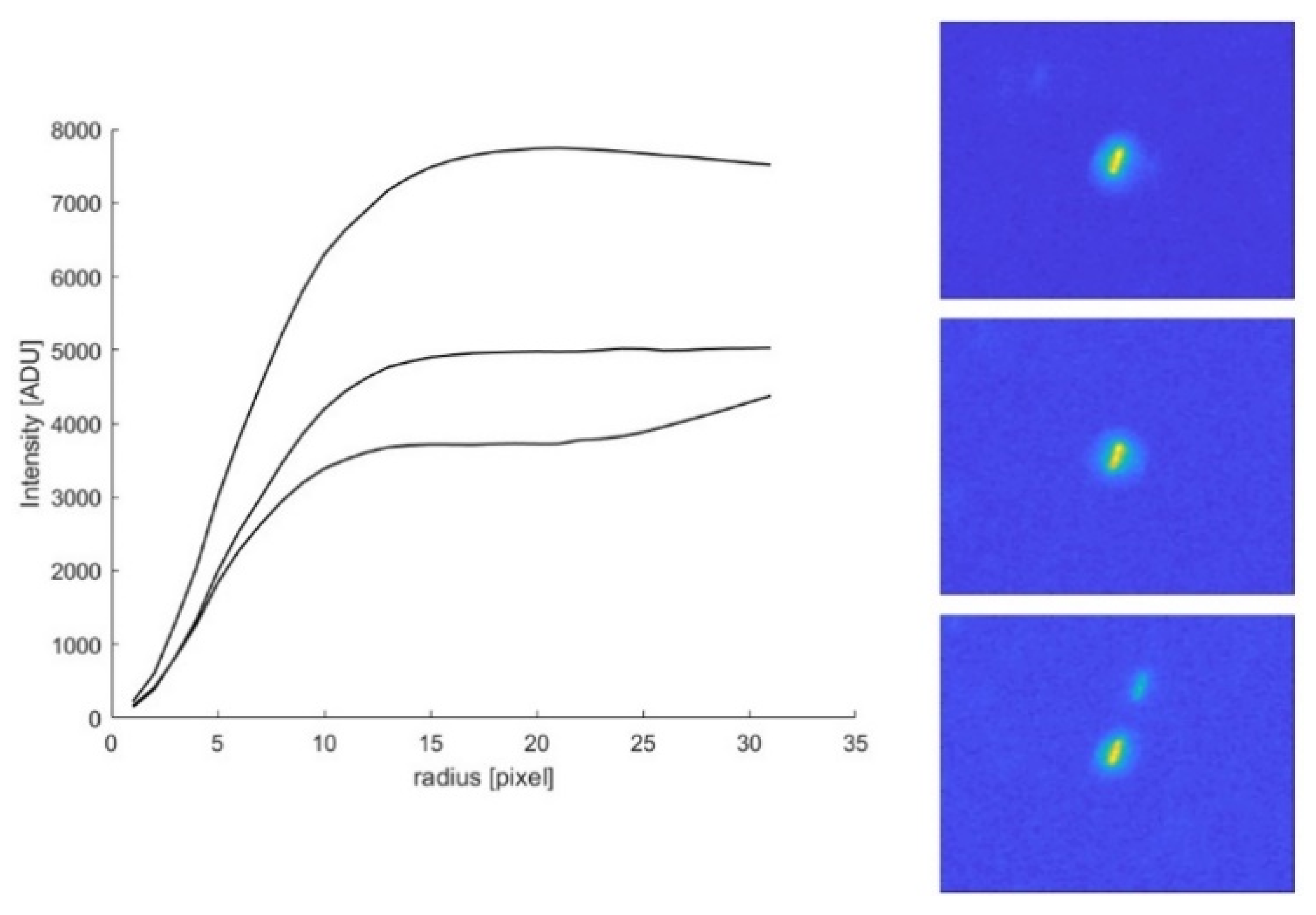
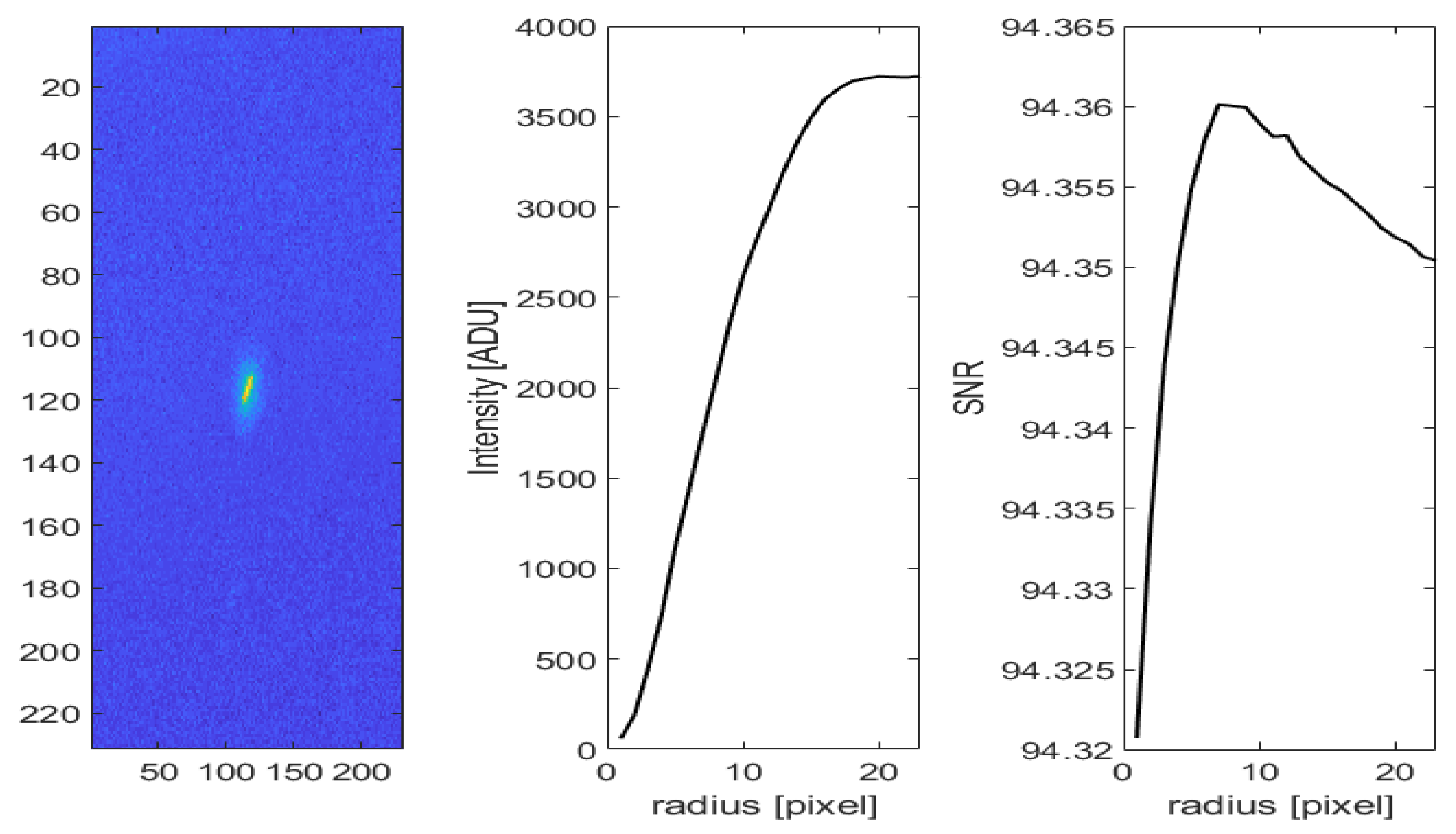
3.2. Star Intensity and Background Estimation

The estimation of the background level makes it possible to correct the fact that the same pixels that collect photons of the object also collect photons from the sky. A common technique is to place a software annulus around the object with a total number of pixels of about three times the number contained within that of the source aperture. For the pixels of the sky annulus, the median intensity is found and then all those with values greater than ± 3 σ from the median are tossed out. With this cut-off the cosmic ray hits, bad pixels, and astronomical neighbors’ contamination are eliminated. The cut-off technique is repeated another time with the new distribution. Finally, the background level is the median value of the final histogram [32].
For calculation of the star intensity, a software aperture of star dependent radius is centred on the pixel coordinate of the star and then the pixels in this area (A) are summed; this is the total integrated photometric source signal (S). To remove the background, the following formula is applied:
I =   S n p i x B ¯
where n p i x is the total number of pixels contained within the area A and B ¯ is the background level discussed above. With this value, it is possible to exclude all the stars that are saturated.
It has been shown by Howell that there exists a relation between the radius of the aperture of the star and the signal-to-noise ratio obtained for that measurement. An optimum of the radius aperture, that is, one that provides the optimum or best signal-to-noise ratio for the measurement, can be determined and generally has a radius of near 1 · FWHM. This optimum radius is a weak function of the source brightness, becoming smaller in size for fainter sources. When the optimum star radius is found, it is possible to calculate the intensity of the star using this radius [31,32]. The Figure 2 and Figure 3 show, respectively, the growth curve, i.e., the variation of the star intensity with respect to the radius, for three different stars and, for the better one, the Signal to Noise Ratio (SNR) trend with respect to the radius.
In the following example, it is shown how the mean and the standard deviation of the error in magnitude change according to a different value of the radius used for each star in each frame. The analysed video is the same used in Section 3.1 and a minimum in the standard deviation occurs for r = 3, as shown in Figure 4. This radius is the optimum value for this video. The optimum radius does not assume the same value for each video, since it depends on several factors: the stars present in Field of View (FoV), the seeing, and the characteristics of the sensor.

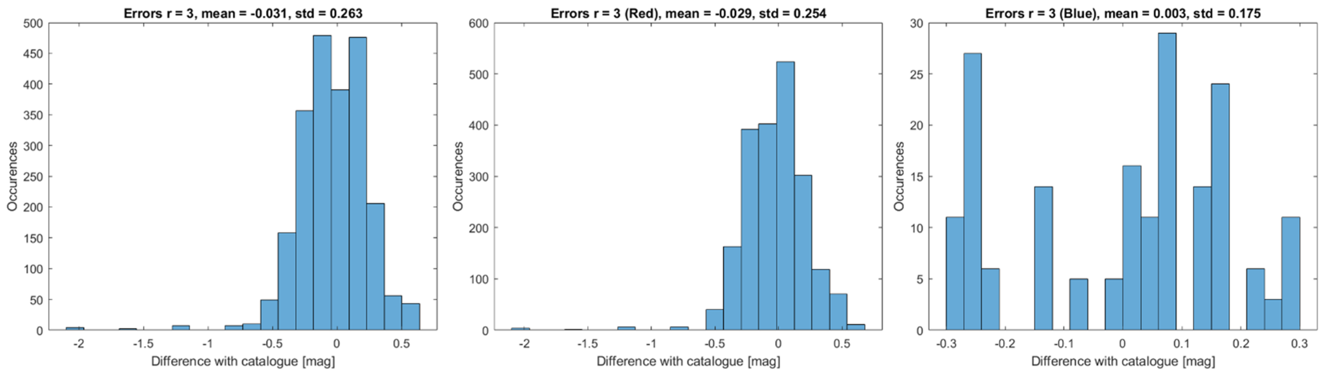
3.3. Stars Magnitude

The previous procedure calculates the intensity of each star present in the field of view for each frame. Therefore, the intensity of each star is obtained as a function of time. Since the object is being chased, the latter will be stationary in the field of view, while the stars will move. Therefore, the same stars will not always be present during the entire recording of the object. The object video is then divided into time intervals. In each interval, only the stars that are present in the entire length of the interval are chosen. The intensity of the star is approximated as a constant that is equal to the median of the intensities that the star assumes in that interval. At this point, the apparent magnitude of each star present in the interval is calculated with respect to all the others present in the same interval by:
m a g s t a r i = m a g s t a r j _ c a t 2.5 log ( I s t a r i I s t a r j )
for i,j = 1,…,Nstar and i≠j where magstar,i is the magnitude of the i-th star, magstar,j_cat is the catalogue magnitude of the j-th star, Istar,i is the intensity of the i-th star in ADU and Istar,j is the intensity of the j-th star in the ADU. For each star, therefore, a vector of possible apparent magnitudes is obtained, and it is assumed that the apparent magnitude of the star is equal to the median of these values. In each interval, there is a certain number of stars n, which is combined in groups of m, with m ≤ n, in order to find the combination of m stars that minimizes the standard deviation of the measurements. The set of combinations of stars chosen for each interval represents the list of stars that will be used as references for calculating the magnitude of the object being tracked. In Figure 5, it is shown how the proposed method improves the magnitudes’ estimation.

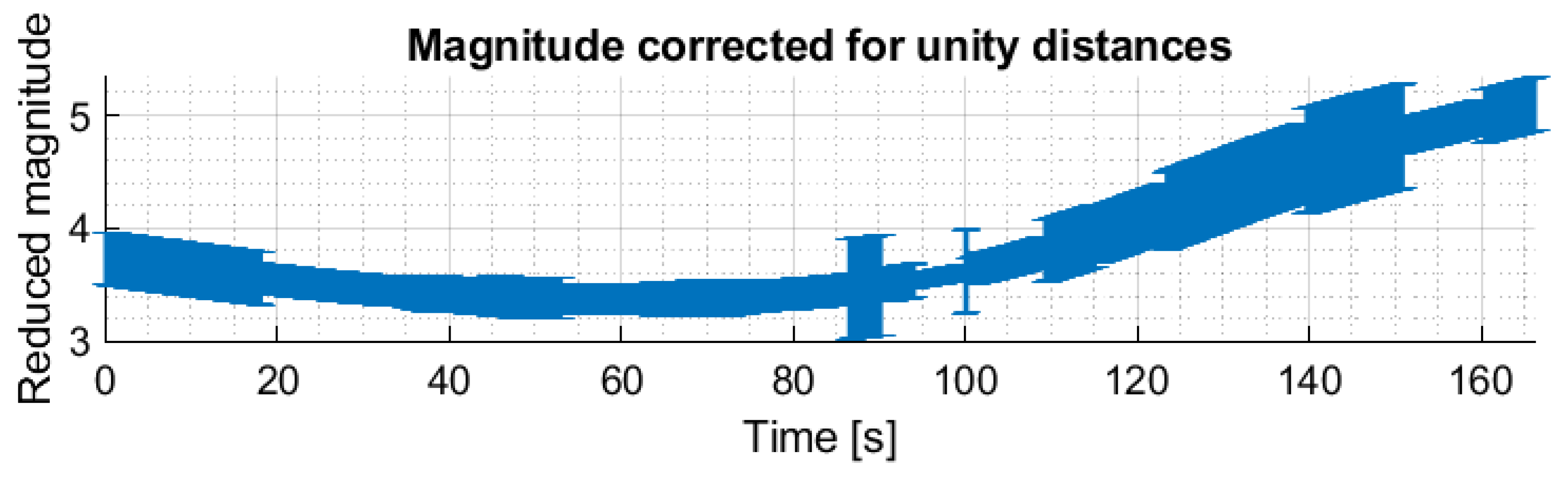
3.4. Object Magnitude Variation

To calculate the change in magnitude of the tracked object over time (light-curve), it is necessary to calculate the intensity of the object in each frame. If the object is not perfectly still in the field of view during the recording, as often happens, it is necessary to use an algorithm that determines the pixel coordinates of the object center in each frame. Once the coordinates of the object in each frame have been obtained, it is possible to calculate the intensity of the object as described in Section 3.2 and consequently its magnitude, as described in the previous section, using as reference those stars that result from the optimization process. In Figure 6, the flowchart of the software for the video analysis is shown.
In Phase 1, each frame of the video is analyzed individually. It consists in initializing some parameters that are useful for the following phases: frame intervals that the user wants to analyze, the object center useful for the subsequent tracking of it, kernel dimensions for the calculation of the object’s intensity and background estimation. The stellar field solved in Phase 2 makes it possible to understand where the sensor is observing in the celestial vault. In this way, the stars present in the field of view are identified in terms of celestial coordinates (RA, Dec), pixel coordinates and magnitude (bolometric and visual). In the third phase, since the pixel coordinates of the stars are known, those at the edges are excluded so that the kernel applied to them does not get out of the image. A spectral analysis occurs in the remaining ones, discriminating them into red and blue stars, so as to choose stars belonging to the same spectral class. Finally, the unsaturated stars are chosen for the calculation of the object’s magnitude. Once the intensity of the stars in the field of view is known, the apparent magnitude of each star is calculated with respect to the others in the field of view in the course of Phase 4. During the whole video, the stars present are not always the same, but some remain for a certain frame interval, and others for other intervals. Then, this analysis is carried out for each frame interval found in which the same stars are always present for the entire duration of that interval. The apparent magnitude of each star is calculated as the median value of the magnitudes of that star with respect to the others. For each frame interval, every single star is compared to different groups of other stars, therefore different combinations could occur. The combination of stars that minimizes the standard deviation of the measurements is the one chosen to calculate the apparent magnitude of the object. In the last phase, the object is chased for the entire duration of the video and tracked along its path. Starting from the coordinates entered in Phase 1, the software is able to identify the position of the object frame by frame. Once the flow and background have been calculated, using kernel parameters given as input in Phase 1, it is possible to calculate the intensity of the object over time and therefore its apparent magnitude. If the frames are finished then the software returns the light curve of the object, otherwise it switches to the next frame until the last frame is reached.
The output light-curve does not take into account of the range-rate between the object and the observatory. So, a normalization with respect to the range and Earth’s radius is necessary. In particular, the normalization used must take into account the distance between the observatory and the satellite, thus eliminating the trend due to the range, but must not modify the average value of the object’s magnitude. Several normalization procedures have been tried, and the one that was more efficient, according to the criteria described above, can be expressed by the following formula:
M R = M 5 log 10 ( r R t m a x ( r R t ) )
where MR is the normalized magnitude, which is called reduced magnitude, M is the object’s magnitude without normalization, r is the range and Rt is the Earth’s radius that is used as a scale factor for the range. The result of the normalization procedure is shown in Figure 7 and Figure 8.
The decrease and the increase in the magnitude values, respectively, at the start and at the end of the tracking, represent the rise and the sets of the object.

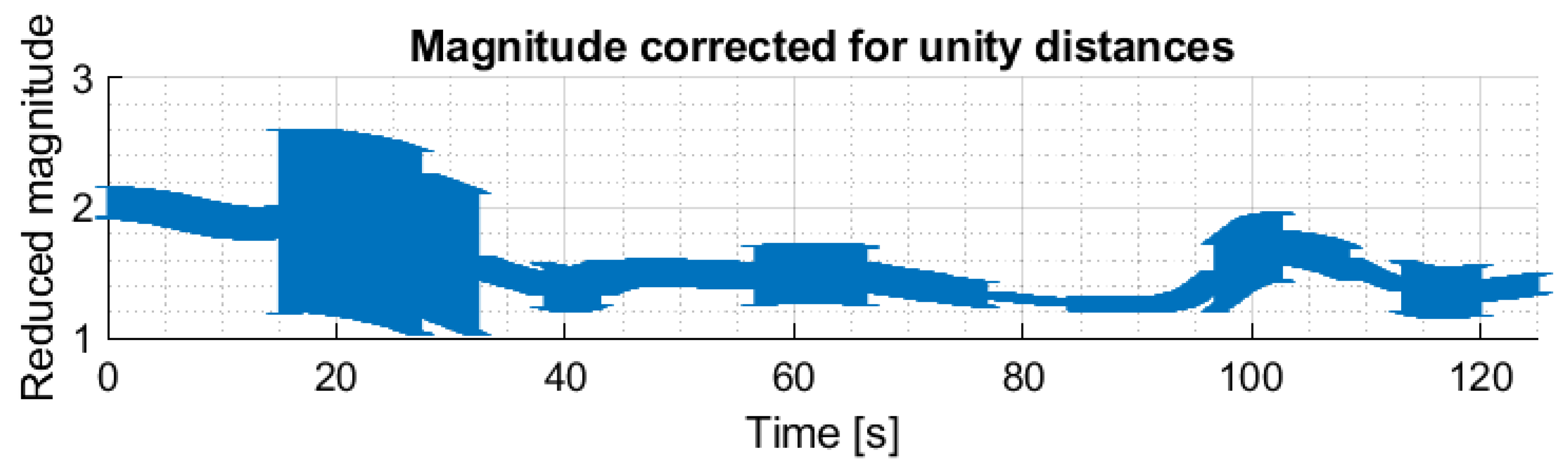
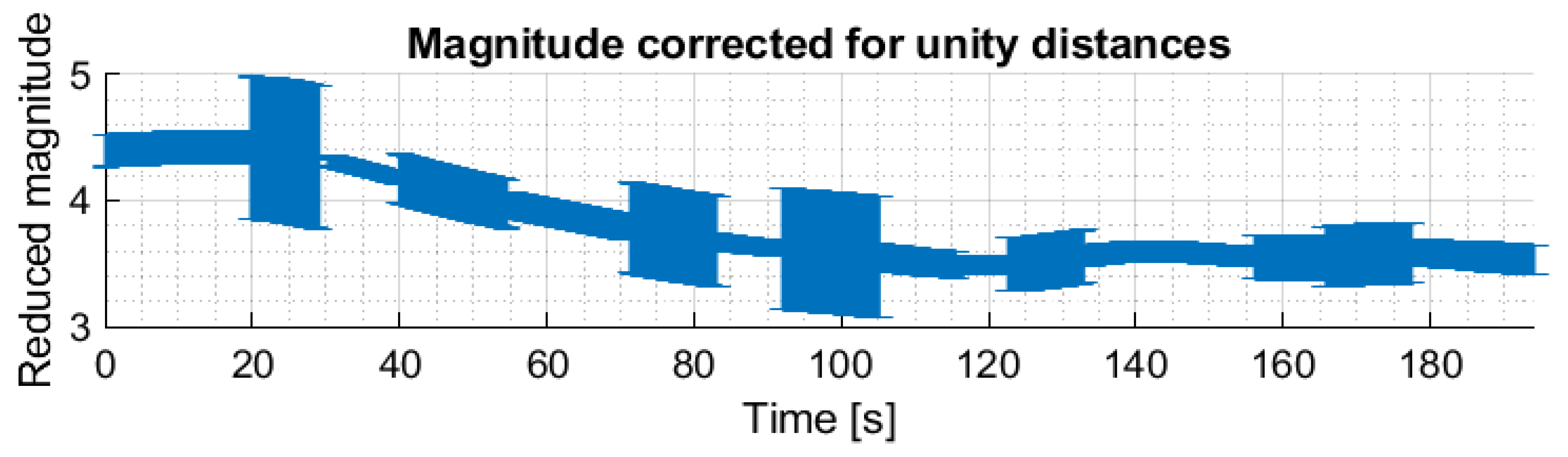
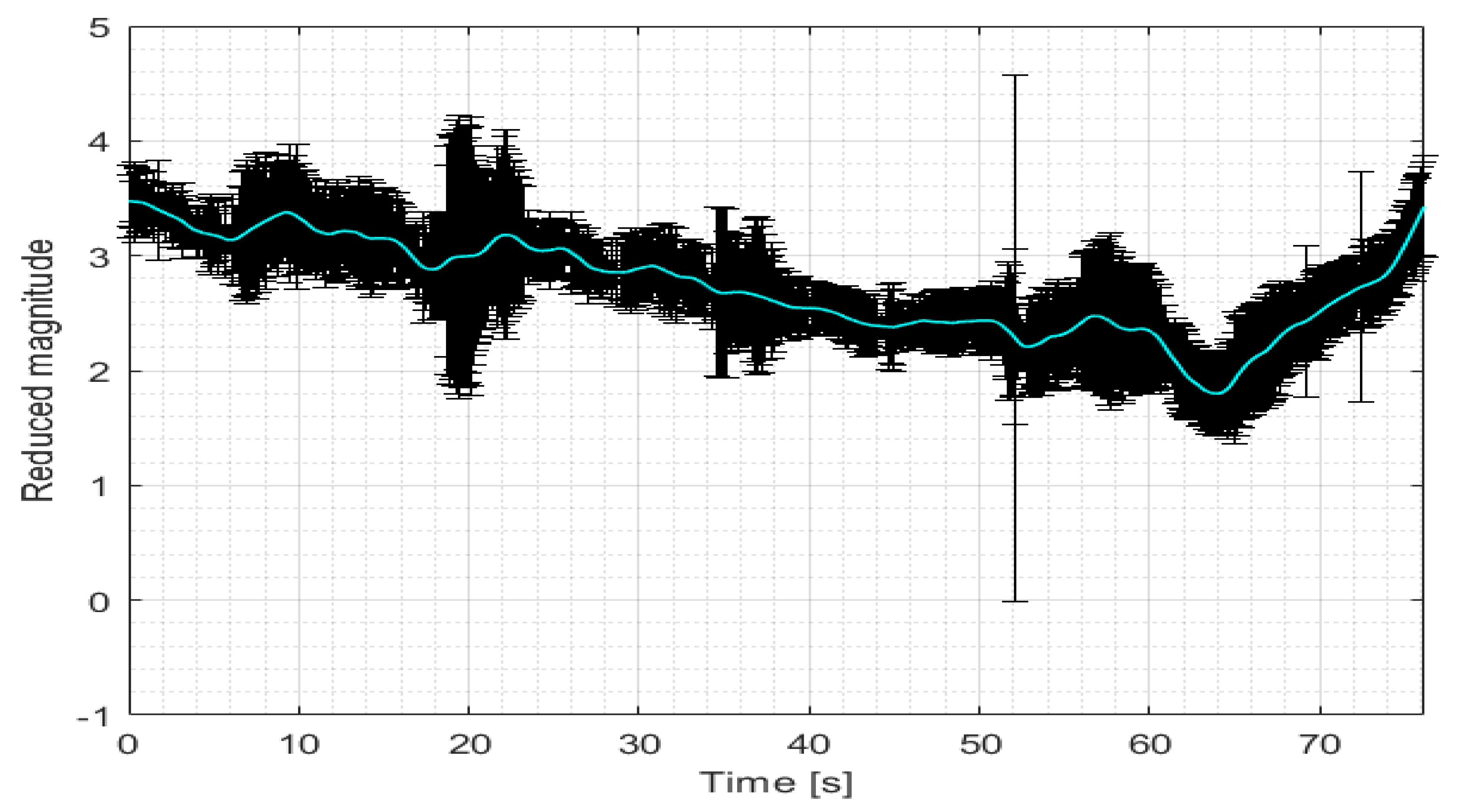
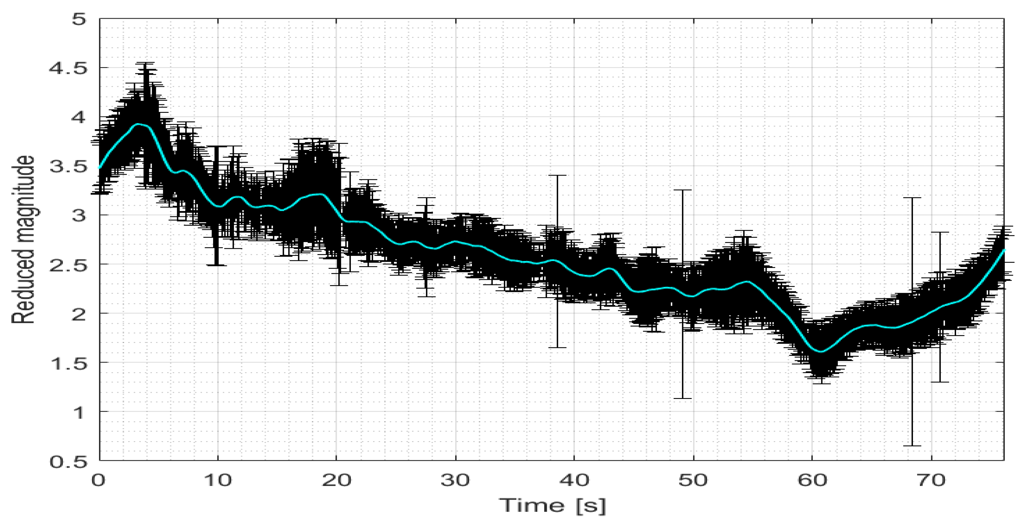
3.5. Light-Curves Examples

To find the optimal shooting parameters, many tests were carried out. Mainly, it is necessary to check the binning, the exposure time, the frame rate, the image type (8, 12 or 16 bit) and whether to use global or rolling shutter. The main parameter to take under control is the exposure time, since an overly high value of this means that the stars in the field of view are represented by overly long strips with consequent failure in the resolution of the star field. Conversely, if an overly short exposure time is used, not enough stars are identified for the astrometric resolution. Regarding the object, a high exposure time value could lead to a saturation of the pixels that represent the object in the field of view. Instead, a low exposure time value involves a lower signal to noise ratio of the object that prevents it from being visible.
In Figure 9, Figure 10 and Figure 11 some examples are shown of the light-curves taken both from RESDOS and SCUDO observatories recorded within the Inter-Agency Space Debris Coordination Committee (IADC) campaign WG1 AI 38.2, “Attitude motion characterization of LEO upper stages using different observation techniques” [33], useful to validate the light-curve analysis software. From these examples, it is possible to see how the tumbling motion of these objects is quite smooth, showing a repetition period even if the passage is longer. The errors represented changes depending on the actual state of the sky observed, so the error bars accommodate, for every single measure, the real observation situation.
Many tests were needed to calibrate the software parameters to obtain a correct calculation of the magnitude of the stars and the object and also to correctly follow the objects in the video frames. Once the software was validated, a simultaneous observation test was pursued. Figure 12 and Figure 13 show an example of light-curves obtained during a bi-static observation taken from RESDOS and SCUDO observatories. The object under consideration is the satellite ATLAS 2AS CENTAUR (SSN 28096) during its passage above Italy, which occurred on the 30/10/2020 at 19:29:00 UTC. It is possible to notice how, even if the main behavior is similar, some small differences are representative of different attitudes of reflective faces with respect to the two observatories. These differences are of paramount importance in the process of light-curve inversion that is discussed later.

4. Attitude Reconstruction

An object’s magnitude may be directly measured using optical instruments through the light curve analysis [34,35,36]. The attitude determination issue is fundamental in order to understand the behavior of orbiting objects, above all for the uncontrolled one. In particular, the knowledge of the attitude of a debris object is critical during the re-entry phase. Here, the atmosphere plays an important role in the evolution of the object’s descent given its interaction with the object’s surface. In this section, a method for attitude reconstruction will be explained.

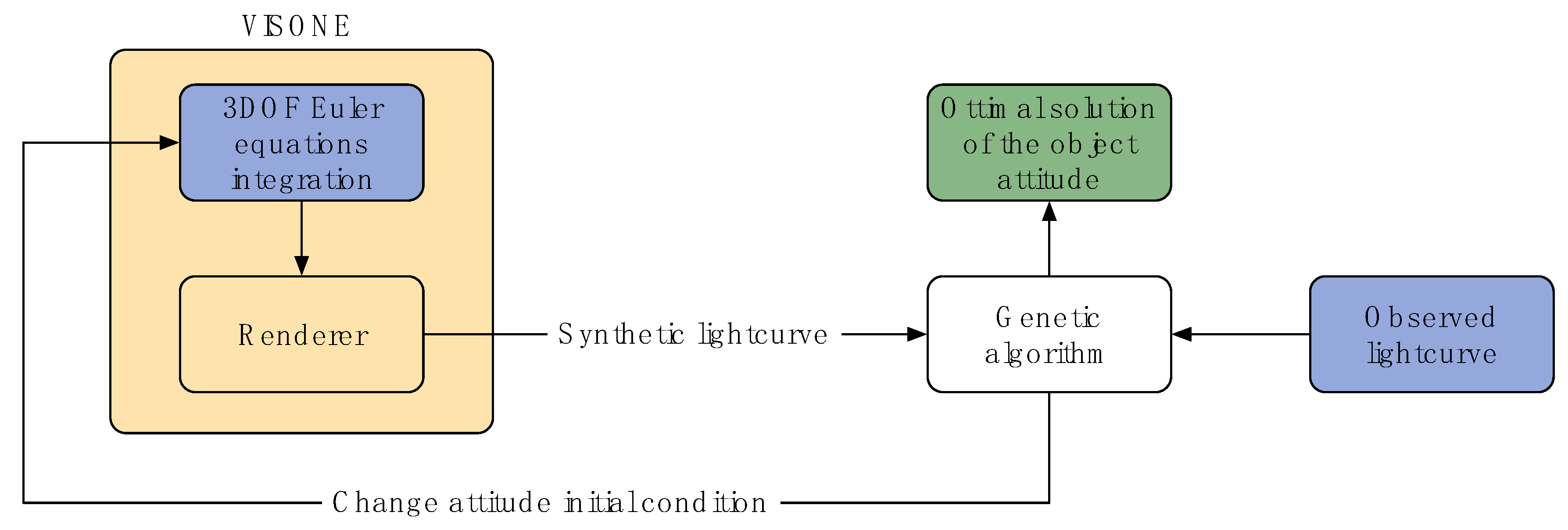
4.1. Overview of the Method

Once the observed light-curve is retrieved from an optical observation, the next step is to compare it with a synthetic one in order to retrieve the object’s attitude. Many synthetic light-curves are generated with different initial attitude parameters. The more the synthetic light-curve is similar to the observed one, the greater the likelihood that the corresponding attitude parameter represents the real object’s attitude. The critical phase, in the whole process, is the synthetic light-curve generator: it must be as realistic and reliable as possible both from the optical and physical point of view.
First, an SGP-4 (Simplified General Perturbation) routine in the interval of interest occurs to retrieve the object orbit [4]. Moreover, the observer and the sun position are computed for each instant in the same object’s reference frame.
A 3D model of the object is needed to generate a synthetic image of it over time. The artificial light-curve is the result of the flux of light reflected by the object, intends as the sum of the pixel of the image. Later, a genetic algorithm is used to minimize a cost function defined as the difference between the real light-curve and the synthetic one. The algorithm tries different initial attitude parameters until both curves are comparable. In the next sections, the whole process will be explained in detail.

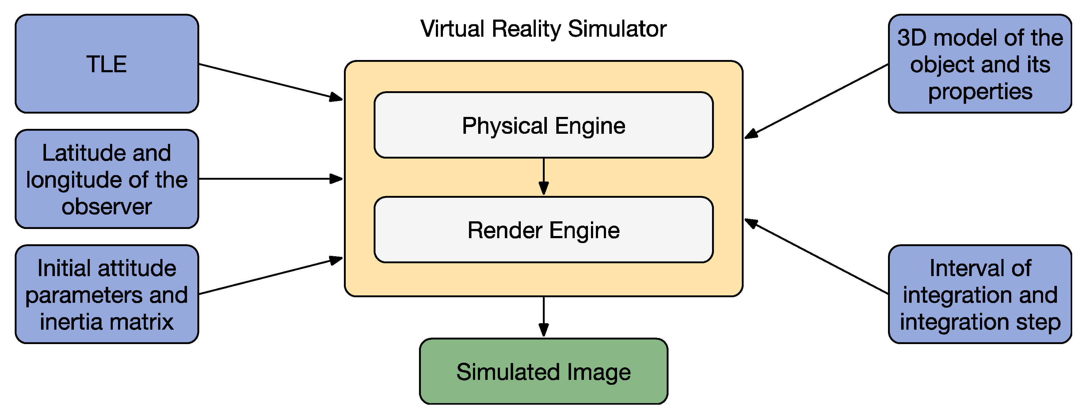
4.2. Virtual Reality Simulation

As mentioned above, the crucial phase is to generate an accurate model of the object and so an as accurate representation as possible of the light reflected by the object (light-curve). To do this, a virtual reality simulation is implemented; many parameters and variables, both from the optical and physical point of view, have to be taken into account such as the atmospheric extinction, the object’s shape and materials, the phase angle between sun–object–observer in order to obtain the light reflected by each part of the object and to accurately reproduce the shadow areas cast by the object on itself. A bad estimate of these parameters leads to an inaccurate synthetic light-curve and therefore to an imprecise attitude determination. In this context, a virtual reality engine was developed specifically for space observation simulations: the Virtual Space Observation Engine (VISONE). Two different modules can be found in the software: the Physical Engine and the Rendering Engine. Figure 14 shows a schematic of the VISONE engine.

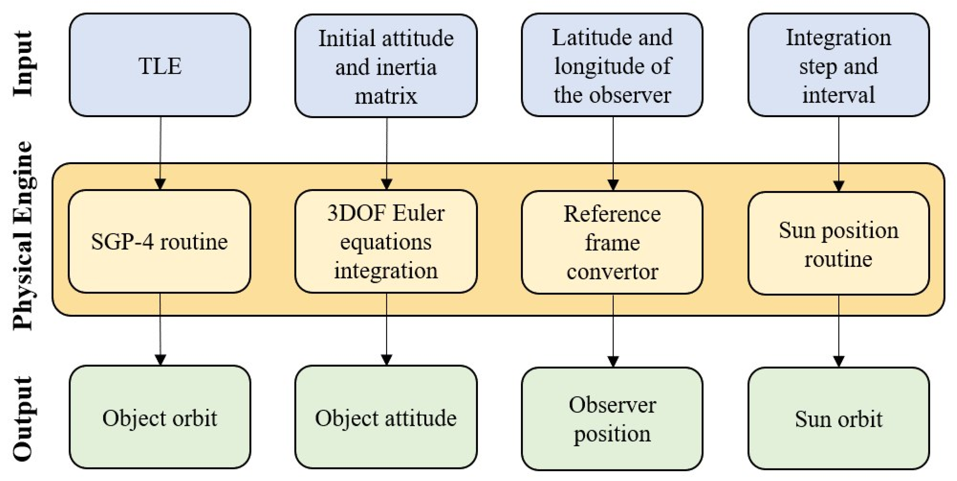
4.2.1. Physical Engine

This part of the software has the task of study the physic of the problem. In particular, to obtain a simulation of the light reflected by the object that is as realistic as possible, it is necessary to compute, instant by instant:
  • Orbital position;
  • Attitude;
  • Observer position (i.e., ground station);
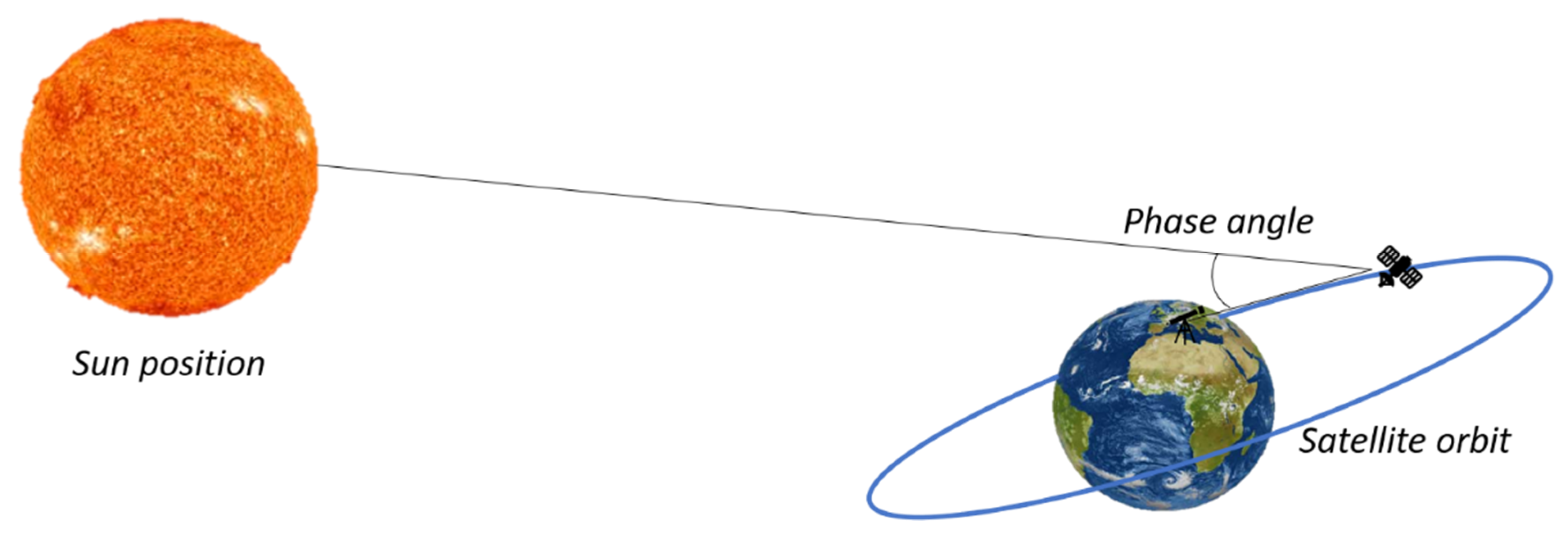
  • Position of the sun.
All these parameters make it possible to compute the phase angle, see Figure 15, which is fundamental for the computing of the amount of light reflected by the object.
The position of the object, for each instant of time, is computed using an SGP-4 [4] routine, that takes as input the TLE of the object. As mentioned in the introduction, the TLEs are characterized by low accuracy and short reliability that can lead to errors of several km in the satellite position [5]. This means that a TLE loses its utility in a few days. Moreover, in the case of a re-entering object, for which the light-curve plays a fundamental role in the re-entry prediction, the reliability period decreases to a few hours. Therefore, the TLE closest to the measured time is chosen. While the ground station position is well known, the sun position is computed using the ephemeris. It is essential that all these positions are expressed in the same reference system, e.g., the Earth-Centered Inertial (ECI) one. Figure 16 shows the Physical Engine structure.
Regarding the dynamic state of the object, the classical Euler equation for a rigid body is used under the acceptable hypothesis of the null external torque since their effects on the object are negligible during the light-curve acquisition period. Here, the dynamic state is represented by the Euler angle and the angular velocity components in the satellite reference frame (φ0, θ0, ψ0, p0, q0, r0). A specific matrix of inertia is considered for every type of object in order to consider the different geometry.

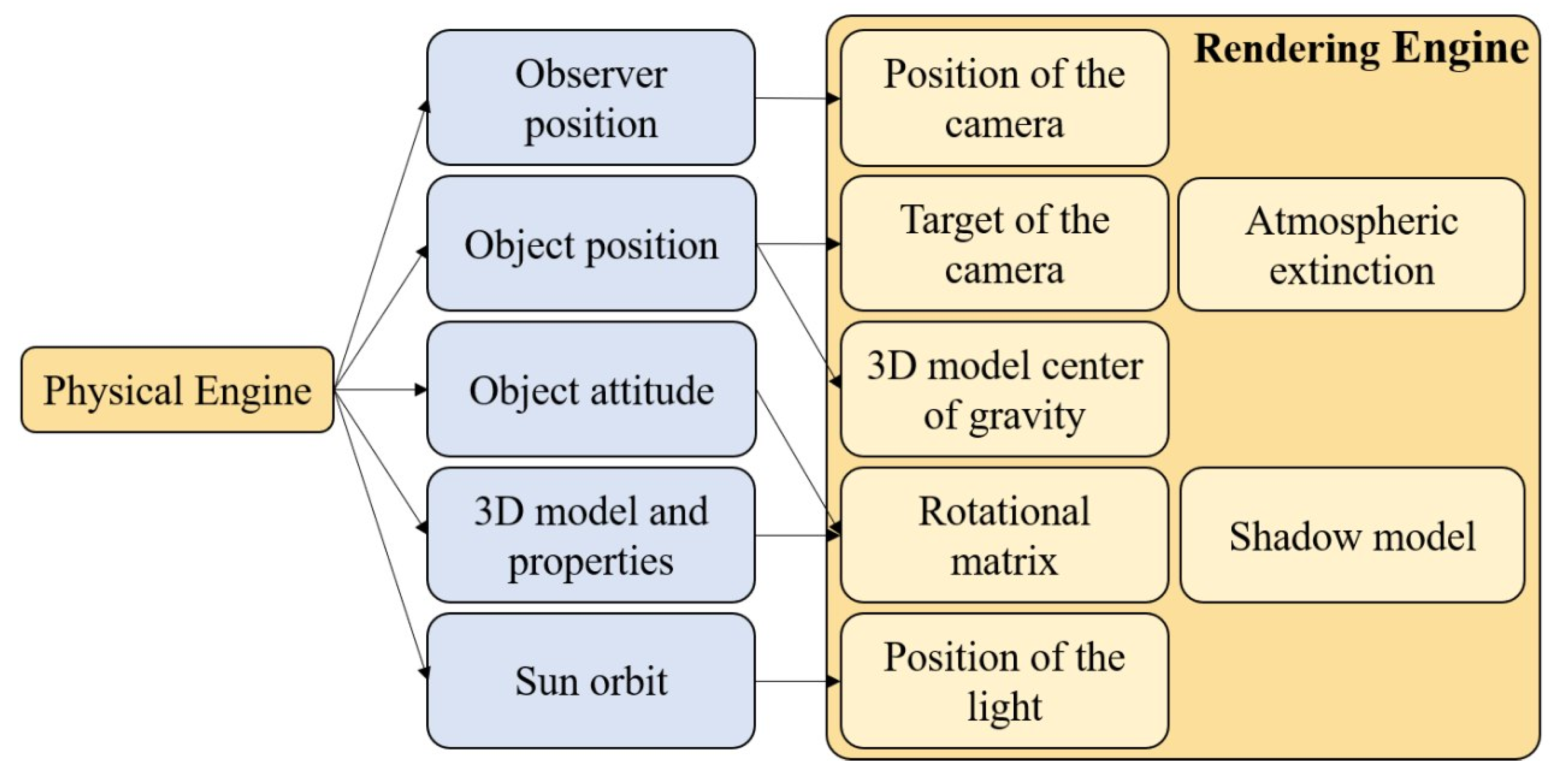
4.2.2. Rendering Engine

The second step to retrieve the attitude is the Rendering Engine. In this step, the aim is to recreate a synthetic image of the object as realistically as possible. With this purpose, the output of the Physical Engine will be the input of the rendering one. In the Rendering Engine, new parameters such as atmospheric extinction, the object’s shape and materials, and the direction of the sunlight, must be considered. Since the engine must accurately reproduce the shadow on the object’s surface due to its components, e.g., solar panels, or antenna, the worse the synthetic image quality, the worse the light-curve quality is, leading to poor results in terms of attitude determination. Indeed, shadows and reflected lights, e.g., by the antenna, create valleys and peaks in the shape of light-curves. In Figure 17, the result of the rendering is shown.
The developed software uses the well-known loader library Assimp [37], which makes the software able to work with most of the material properties used in the 3D rendering field. The Blinn’ Phong light model [38] is used to recreate lighting conditions, whereas the shadows’ areas are modelized following the exponential shadow mapping model [39]. All these choices make it possible to be fast and precise in the light source computation, be they directional or far away, and in the evaluation of the light reflected by the object. The results are shown in the previous figure.
In Figure 18, it can be seen how the Rendering Engine uses the data computed by the physical engine, and it also shows the correspondence between the real parameters and the model parameters.

4.3. Automatic Attitude Determination

The real light-curve, obtained as mentioned in Section 3, depends only on the time t; therefore, it can be defined as IT(t). Instead, the synthetic one generated by VISONE depends not only on the time, but also on the initial attitude condition in terms of Euler angles and angular velocity components. Let φ0, θ0, ψ0 be the initial Euler angles and let p0, q0, r0 be the initial angular velocities. The synthetic light-curve IS can be defined as:
              I S ( t ,   φ 0 ,   θ 0 ,   ψ 0 ,   p 0 ,   q 0 ,   r 0 )
Therefore, it is possible to define a cost function as the the sum over time of the modulus of the difference between the real and the synthetic light-curve:
|   I T ( t )   I S ( t , φ 0 ,   θ 0 ,   ψ 0 ,   p 0 ,   q 0 ,   r 0 ) |
In this way, the issue is reduced to a minimization problem in which the final task is to find the initial attitude parameters that generate the synthetic light-curve that is as close as possible to the real one. Those parameters will be the presumable attitude parameters of the observed object. In this context, a genetic algorithm [40] to solve the problem defined in Equation (5) is used. In addition, it is possible to define validity ranges for each parameter or lock or release parts of the object, such as the movement of the solar panels. This makes it possible to improve both the solution of the attitude when prior information about the attitude of the observed object is known (e.g., solar panels point towards the Sun or the main body point to the nadir) or both in the case of re-entering objects. Figure 19 shows the optimization architecture.

4.4. Method Validation

In order to evaluate the proposed method, two kind of tests werecarried out: the first one was for checking the quality and the accuracy of the method on a groundtruth of synthetic datasets, and the latter instead was for validating the method in a real case.

4.4.1. Synthetic Data

The algorithm was tested on synthetic data in order to check the reliability of the procedure. Once the initial attitude parameters were defined, a white noise was applied on the synthetic light-curve. The resulting synthetic light-curve is given as the target to the algorithm, which returns the attitude parameters that have created it. In Figure 20, the synthetic target light-curve and the found ones are shown. In the Table 2, the real attitude’s initial parameters and the ones found by our method are shown. This result shows how the proposed method has good performance and reliability also in the case of noise. The difference between the target and synthetic parameters reported in Table 2 is due to the optimization process. Each parameter affects the attitude, and so the resulting light-curve is affected in the same way. Nevertheless, the choices made by the genetic algorithm during the optimization process may affect the precision of the parameters found as well as the time it takes to find them. The more the optimizer is left to find the solution, the more the solutions can be corrected.

4.4.2. Real Case Test

In order to test the proposed method on real data, the re-entry campaign in the winter of 2017–2018 of the chinese space station Tiangong-1 was choosen. In Figure 21, the light-curve of the Tiangong-1 passing over Rome on the 15/02/2018 is shown. The light-curve was sampling at 24 fps with a video recording duration of 71 s. The observed light curve (in blue in Figure 21) is very noisy. These fluctuations are caused by the observational method (not entirely optimal) and by the algorithm that determines the flow of light reflected by the object by analyzing the image. Indeed, it seems to be unrealistic that a passive object (i.e., that only reflected the sunlight) varies its intensity in only 1/24 of a second. It is more interesting to see how, even in the presence of noise, the algorithm is able to find those parameters that generate a light-curve similar to the observed one discarding the noise.
In the real case, since the SGP4 routine only provides a prediction of the object’s position, which could differ from the real one due to a time shift, an additional delay parameter is added to the cost function (Equation (5)) to cope with this kind of error. Moreover, in this particular case, another parameter was added to the cost function to take into account a further degree of liberty due to the rotation of the solar pannel with respect to the principal body.
Analyzing the result, the attitude parameters found show that the station seems to have: the x-axis pointed to the velocity vector; the y-axis pointed to the Nadir with an angle between the solar panels and the Sun of about 24°. This configuration creates a drag area, with respect to the velocity vector, of about 48 mq. The attitude parameters found by the proposed method are in line with the community consensus regarding the presumable attitude of the station in that period of time [41,42,43].

5. Conclusions

In this paper, an in-depth method to retrieve light-curve has been shown. Despite the noise of the sCMOS sensor used for optical observation, the results prove that is possible to obtain a light-curve by means of an optical system. To obtain these results, star field resolution was performed in order to find the reference stars on which to calculate the object’s magnitude. Moreover, an optimization process that minimized the standard deviation with respect to several photometric parameters occurred. The whole process has been applied to a bi-static optical system, making it possible to obtain simultaneous data.
Furthermore, a system for the light-curve inversion based on a stochastic optimization (genetic algorithm) was identified, implemented, and tested on the real case of the Tiangong-1. The obtained results show that the method can be used for future re-entry objects.

Author Contributions

G.Z. and S.H.H. worked on the observations segment using RESDOS and SCUDO observatories respectively. L.M. developed the software for the video analysis in order to retrieve light-curves. L.P. worked on the development of the attitude reconstruction software. F.P. and F.S. supervise the whole job, working both in observation activities and software development. All authors have read and agreed to the published version of the manuscript.

Funding

This research was funded by Regione Lazio: CUP B86C17000230002 and Agenzia Spaziale Italiana: N. 2015-031R.1-2018.

Conflicts of Interest

The authors declare no conflict of interest.

References

  1. ESA. “Space Debris by the Numbers,” European Space Agency. Available online: https://www.esa.int/Our_Activities/Operations/Space_Debris/Space_debris_by_the_numbers (accessed on 28 June 2018).
  2. NSTCC. The National Science and Technology Council Committee on Transportation Research & Development; Interagency Report on Orbital Debris 1995; NSTCC: Washingtong, DC, USA, 1995. [Google Scholar]
  3. Reihs, B.; McLean, F.; Lemmens, S.; Merz, K.; Krag, H. Analysis of CDM covariance consistency in operational collision avoidance. In Proceedings of the 7th European Conference on Space Debris, Darmstadt, Germany, 18–21 April 2017; ESA Space Debris Office: Darmstadt, Germany, 2017. [Google Scholar]
  4. Valladoe, D.A.; McClain, W.D. Fundamentals of Astrodynamics and Applications, 3rd ed.; Microcosm Press/Springer: Hawthorne, CA, USA, 2007. [Google Scholar]
  5. Vallado, D.; Cefola, P. «Two-line element sets-Practice and use». In Proceedings of the 63rd International Astronautical Congress, Naples, Italy, 1–5 October 2012; IAF: Paris, France, 2012. IAC-12,C1,6,12,x13640. Volume 7, pp. 5812–5825. [Google Scholar]
  6. MehtaiD, P.M.; Kubicek, M.; Minisci, E.; Vasile, M. Sensitivity analysis and probabilistic re-entry modeling for debris using high dimensional model representation based uncertainty treatment. Adv. Space Res. 2017, 59, 193–211. [Google Scholar] [CrossRef] [Green Version]
  7. Acernese, M.; Zarcone, G. Improving accuracy of LEO objects Two-line elements through optical measurements. In Proceedings of the 69th International Astronautical Congress, Bremen, Germany, 1–5 October 2018. IAC-18,A6,9,8,x47421. [Google Scholar]
  8. DiPrima, F.; Santoni, F.; Piergentili, F.; Fortunato, V.; Abbattista, C.; Amoruso, L. Efficient and automatic image reduction framework for space debris detection based on GPU technology. Acta Astronaut. 2018, 145, 332–341. [Google Scholar] [CrossRef]
  9. Scire, G.; Piergentili, F.; Santoni, F. Spacecraft Recognition in Co-Located Satellites Cluster through Optical Measures. IEEE Trans. Aerosp. Electron. Syst. 2017, 53, 1699–1708. [Google Scholar] [CrossRef]
  10. Piergentili, F.; Santoni, F.; Seitzer, P. Attitude Determination of Orbiting Objects from Lightcurve Measurements. IEEE Trans. Aerosp. Electron. Syst. 2017, 53, 81–90. [Google Scholar] [CrossRef]
  11. Cardona, T.; Seitzer, P.; Rossi, A.; Piergentili, F.; Santoni, F. BVRI photometric observations and light-curve analysis of GEO objects. Adv. Space Res. 2016, 58, 514–527. [Google Scholar] [CrossRef]
  12. Santoni, F. Dynamics of Spring-Deployed Solar Panels for Agile Nanospacecraft. J. Aerosp. Eng. 2015, 28, 04014122. [Google Scholar] [CrossRef]
  13. Santoni, F.; Piergentili, F. Analysis of the UNISAT-3 Solar Array In-Orbit Performance. J. Spacecr. Rocket. 2008, 45, 142–148. [Google Scholar] [CrossRef]
  14. Graziani, F.; Santoni, F.; Piergentili, F.; Bulgarelli, F.; Sgubini, M.; Bernardini, S. Manufacturing and Launching Student-Made Microsatellites: “Hands-on” Education at the University of Roma. In Proceedings of the 55th International Astronautical Congress of the International Astronautical Federation, the International Academy of Astronautics, and the International Institute of Space Law, Vancouver, BC, Canada, 4–8 October 2004; IAF: Paris, France, 2004. [Google Scholar] [CrossRef]
  15. Vaccari, L.; Altissimo, M.; Di Fabrizio, E.; De Grandis, F.; Manzoni, G.; Santoni, F.; Graziani, F.; Gerardino, A.; Pérennès, F.; Miotti, P. Design and prototyping of a micropropulsion system for microsatellites attitude control and orbit correction. J. Vac. Sci. Technol. B Microelectron. Nanometer Struct. 2002, 20, 2793. [Google Scholar] [CrossRef]
  16. Marzioli, P.; Curiano, F.; Picci, N.; Piergentili, F.; Santoni, F.; Gianfermo, A.; Frezza, L.; Amadio, D.; Acernese, M.; Parisi, L.; et al. LED-based attitude reconstruction and back-up light communication: Experimental applications for the LEDSAT CubeSat. In Proceedings of the 2019 IEEE 5th International Workshop on Metrology for AeroSpace (MetroAeroSpace), Torino, Italy, 19–21 June 2019; pp. 720–725. [Google Scholar]
  17. Menchinelli, A.; Ingiosi, F.; Pamphili, L.; Marzioli, P.; Patriarca, R.; Msc, F.C.; Piergentili, F. A Reliability Engineering Approach for Managing Risks in CubeSats. Aerospace 2018, 5, 121. [Google Scholar] [CrossRef] [Green Version]
  18. Marzioli, P.; Gugliermetti, L.; Santoni, F.; Delfini, A.; Piergentili, F.; Nardi, L.; Metelli, G.; Benvenuto, E.; Massa, S.; Bennici, E. CultCube: Experiments in autonomous in-orbit cultivation on-board a 12-Units CubeSat platform. Life Sci. Space Res. 2020, 25, 42–52. [Google Scholar] [CrossRef]
  19. Hossein, S.H.; Acernese, M.; Cardona, T.; Cialone, G.; Curianò, F.; Mariani, L.; Marini, V.; Marzioli, P.; Parisi, L.; Piergentili, F.; et al. Sapienza Space debris Observatory Network (SSON): A high coverage infrastructure for space debris monitoring. J. Space Saf. Eng. 2020, 7, 30–37. [Google Scholar] [CrossRef]
  20. Santoni, F.; Piergentili, F.; Cardona, T.; Curianò, F.; Diprima, F.; Hossein, S.H.; Canu, C.; Mariani, L. EQUO-Equatorial Italian Observatory at The Broglio Space Center For Space Debris Monitoring. In Proceedings of the 68th International Astronautical Congress, Adelaide, Australia, 25–29 September 2017. IAC-17,A6,IP,10,x38808. [Google Scholar]
  21. Piergentili, F.; Ceruti, A.; Rizzitelli, F.; Cardona, T.; Battagliere, M.L.; Santoni, F. Space Debris Measurement Using Joint Mid-Latitude and Equatorial Optical Observations. IEEE Trans. Aerosp. Electron. Syst. 2014, 50, 664–675. [Google Scholar] [CrossRef]
  22. Piattoni, J.; Ceruti, A.; Piergentili, F. Automated image analysis for space debris identification and astrometric measurements. Acta Astronaut. 2014, 103, 176–184. [Google Scholar] [CrossRef]
  23. Porfilio, M.; Piergentili, F.; Graziani, F. Two-site orbit determination: The 2003 GEO observation campaign from Collepardo and Mallorca. Adv. Space Res. 2006, 38, 2084–2092. [Google Scholar] [CrossRef]
  24. Scire, G.; Santoni, F.; Piergentili, F. Analysis of orbit determination for space based optical space surveillance system. Adv. Space Res. 2015, 56, 421–428. [Google Scholar] [CrossRef]
  25. Piergentili, F.; Ravaglia, R.; Santoni, F. Close Approach Analysis in the Geosynchronous Region Using Optical Measurements. J. Guid. Control. Dyn. 2014, 37, 705–710. [Google Scholar] [CrossRef]
  26. Siccardi, M. About Time Measurements. In Proceedings of the IEEE 2012 European Frequency and Time Forum (EFTF), Gothenburg, Sweden, 23–27 April 2012. [Google Scholar]
  27. Hogg, D.W.; Blanton, M.; Lang, D.; Mierle, K.; Roweis, S. Automated Astrometry, Astronomical Data Analysis Software and Systems XVII. Available online: http://adsabs.harvard.edu/full/2008ASPC..394...27H (accessed on 12 December 2020).
  28. Høg, E.; Fabricius, C.; Makarov, V.V.; Urban, S.; Corbin, T.; Wycoff, G.; Bastian, U.; Schwekendiek, P.; Wicenec, A. The Tycho-2 Catalogue of the 2.5 Million Brightest Stars; Naval Observatory: Washington, DC, USA, 2000. [Google Scholar]
  29. Olson, T. The Colors of the Stars. In Proceedings of the Color Imaging Conference, Scottsdale, AZ, USA, 17–20 November 1998. [Google Scholar]
  30. Howell, S. Handbook of CCD Astronomy, 2nd ed.; Cambridge University Press: Cambridge, UK, 2006. [Google Scholar]
  31. Howell, S.B. Two-dimensional aperture photometry-Signal-to-noise ratio of point-source observations and optimal data-extraction techniques. Publ. Astron. Soc. Pac. 1989, 101, 616. [Google Scholar] [CrossRef]
  32. Stetson, P.B. On the growth-curve method for calibrating stellar photometry with CCDs. Publ. Astron. Soc. Pac. 1990, 102, 932. [Google Scholar] [CrossRef] [Green Version]
  33. IADC. Inter-Agency Space Debris Coordination Committee. Available online: https://www.iadc-home.org/ (accessed on 1 June 2020).
  34. Fruh, C.; Schildknecht, T. Analysis of observed and simulated light curves of space debris. In Proceedings of the International Astronautical Congress, Prague, Czech Republic, 27 September–1 October 2010. IAC-10.A6.1.9. [Google Scholar]
  35. Bradley, B.; Axelrad, P. Lightcurve Inversion for Shape Estimation of Geo Objects from Space-Based Sensors. In Proceedings of the International Space Symposium for Flight Dynamics, Laurel, MA, USA, 5–9 May 2014. [Google Scholar]
  36. Linder, E. Extraction of Spin Periods of Space Debris from Optical Light Curves. In Proceedings of the International Astronautical Congress, Jerusalem, Israel, 12–16 October 2015. IAC-15,A6,1,2,x29020. [Google Scholar]
  37. Schulze, T.; Gessler, A.; Kulling, K.; Nadlinger, D.; Klein, J.; Sibly, M.; Gubisch, M. Open Asset Import Library (Assimp). January 2012. Computer Software. Available online: https:github.com/assimp/assimp (accessed on 1 October 2020).
  38. James, F. Blinn. Models of light reflection for computer synthesized pictures. In ACM SIGGRAPH Computer Graphics; ACM: New York, NY, USA, 1977; Volume 11, pp. 192–198. [Google Scholar]
  39. Annen, T.; Mertens, T.; Seidel, H.; Flerackers, E.; Kautz, J. Exponential shadow maps. In Proceedings of Graphics Interface; Canadian Information Processing Society: Mississauga, ON, Canada, 2008; pp. 155–161. [Google Scholar]
  40. Ponsich, A.; Azzaro-Pantel, C.; Domenech, S.; Pibouleau, L. Constraint handling strategies in Genetic Algorithms application to optimal batch plant design. Chem. Eng. Process. Process. Intensif. 2008, 47, 420–434. [Google Scholar] [CrossRef] [Green Version]
  41. Vellutini, E.; Bianchi, G.; Pardini, C.; Anselmo, L.; Pisanu, T.; Di Lizia, P.; Piergentili, F.; Monaci, F.; Reali, M.; Villadei, W.; et al. Monitoring the final orbital decay and the re-entry of Tiangong-1 with the Italian SST ground sensor network. J. Space Saf. Eng. 2020, 7, 487–501. [Google Scholar] [CrossRef]
  42. Sommer, S.; Karamanavis, V.; Schlichthaber, F.; Patzelt, T.; Rosebrock, J.; Cerutti-Maori, D.; Leushacke, L. February. Analysis of the attitude motion and cross-sectional area of Tiangong-1 during its uncontrolled re-entry. In Proceedings of the 1st NEO and Debris Detection Conference, Darmstadt, Germany, 22–24 January 2019; ESA Space Safety Programme Office: Darmstadt, Germany, 2019. [Google Scholar]
  43. Pardini, C.; Anselmo, L. Monitoring the orbital decay of the Chinese space station Tiangong-1 from the loss of control until the re-entry into the Earth’s atmosphere. J. Space Saf. Eng. 2019, 6, 265–275. [Google Scholar] [CrossRef]
Figure 1. The figure shows how the mean and the standard deviation of the difference between the catalogued and calculated magnitude, decrease using stars with the same spectral class. On the left is shown the histogram obtained using all the stars present in the video recording, on the center using only the red stars and, on the right, using only the blue stars.
Aerospace 08 00004 g001
Figure 2. Intensity variation with respect to the radius (growth curves) for 3 different stars. The upper curve corresponds to the upper image, the central curve (the only asymptotic stable curve) corresponds to the central image and the lower curve corresponds to the lower image.
Aerospace 08 00004 g002
Figure 3. Star image on the left, growth curve in the center and the SNR curve calculated with the CCD equation in the right. From the last curve, an optimum radius equal to 7 px is found.
Aerospace 08 00004 g003
Figure 4. Optimum radius identification: standard deviation and mean of the error for each radius used for analyzing the example video.
Aerospace 08 00004 g004
Figure 5. Errors mean and standard deviation without stars combination (left) and with stars combination (right).
Aerospace 08 00004 g005
Figure 6. Video analysis software flow chart.
Aerospace 08 00004 g006
Figure 7. Observed light-curve not normalized of CZ-4C (SSN 40879) taken the 22nd of July 2020 from SCUDO observatory.
Aerospace 08 00004 g007
Figure 8. Observed normalized light-curve of CZ-4C (SSN 40879) taken the 22nd of July 2020 from SCUDO observatory.
Aerospace 08 00004 g008
Figure 9. Observed light-curve of CZ-4C R/B (SSN 40879) taken the 20th of July 2020 from SCUDO observatory.
Aerospace 08 00004 g009
Figure 10. Observed light-curve of Cosmos 2322 Rocket (SSN 23704) taken the 25th August 2020 from RESDOS observatory.
Aerospace 08 00004 g010
Figure 11. Observed light-curve of Cosmos 2297 Rocket (SSN 23405) taken the 28th of August 2020 from SCUDO observatory.
Aerospace 08 00004 g011
Figure 12. Observed light-curve of ATLAS 2AS CENTAUR (SSN 28096) taken the 30/10/2020 from RESDOS observatory.
Aerospace 08 00004 g012
Figure 13. Observed light-curve of ATLAS 2AS CENTAUR (SSN 28096) taken the 30/10/2020 from SCUDO observatory.
Aerospace 08 00004 g013
Figure 14. VISONE schematic—some of the input parameters taken by VISONE are: the interval of integration and the time step the 3D model of the object of which we want to find the attitude, its inertia matrix and its initial dynamical state (i.e., initial angle and angular velocity); the last TLE of the object, as well as the position of the observer. VISONE then computes the position of the object and the sun in the same reference frame and renders on an image the 3D model of the orbital object as it should be seen by an observer on Earth.
Aerospace 08 00004 g014
Figure 15. Phase angle—this image shows the phase angle, observer–object–sun, needed to compute the amount of light reflected by the object.
Aerospace 08 00004 g015
Figure 16. Physical Engine—this engine takes care of computing for each time step the position of the orbital object and its dynamical state, taking as input the TLE, the initial state with the inertial matrix. At the same time, the position of the observer and of the sun will be computed in the same integrated interval with the same sampling rate. Moreover, all the results will be given in the same reference frame.
Aerospace 08 00004 g016
Figure 17. Rendered images—this figure shows the result of the rendering engine on the 3D model of the Tiangong-1 and Envisat with shadow [https://sketchfab.com/].
Aerospace 08 00004 g017
Figure 18. Rendering Engine—this engine takes care of computing, for each time step, the synthetic image of the object. The position of the observer is used as the position of the camera. The position of the object is used by the engine as the target of the barycenter of the 3D model to be rendered; the attitude of the object is then used to compute the rotation matrix of the model; finally, the position of the sun is used as the position of the light in the rendering engine.
Aerospace 08 00004 g018
Figure 19. Optimization architecture—the scheme depicts how the proposed method finds the attitude is shown. The genetic algorithm uses the Equation (5) to compare the observed light-curve and the synthetic one. Then, the genetic algorithm changes the initial attitude parameters accordantly, in order to create a new synthetic light-curve. This process is repeated until the best synthetic attitude is found i.e., the presumable object attitude.
Aerospace 08 00004 g019
Figure 20. Synthetic test—. In blue, the synthetic light-curve created with VISONE, while in red the light-curve found by the genetic algorithm are shown.
Aerospace 08 00004 g020
Figure 21. Light-curve of the Tiangong-1 passing over Rome on the 15/02/2018 sampling at 24 fps in blue; in red, the synthetic light-curve found by the proposed method.
Aerospace 08 00004 g021
Table 1. System characteristics.
RESDOS/SCUDO
SensorTypesCMOS
Resolution5.5 Mpx
Sensor Diagonal22 mm
Max Fps100
TelescopeFocal Length750 mm
Diameter150 mm
Mount TypeEquatorial
Table 2. The initial attitude parameters found by the proposed method on a synthetic dataset in comparison with the real one, where φ0, θ0, ψ0 are the Euler angles (in degrees) and p0, q0, r0 the angular velocities (in degrees/sec).
φ0θ0ψ0p0q0r0
Real10.060.0210.05.01.50.5
Found10.561.7209.35.22.70.3
Publisher’s Note: MDPI stays neutral with regard to jurisdictional claims in published maps and institutional affiliations.

