Numerical Simulations on Unsteady Nonlinear Transonic Airfoil Flow


DLR (German Aerospace Center), Institute of Aeroelasticity, Bunsenstr. 10, 37073 Göttingen, Germany
Aerospace 2021, 8(1), 7; https://0-doi-org.brum.beds.ac.uk/10.3390/aerospace8010007
Submission received: 30 October 2020
/
Revised: 15 December 2020
/
Accepted: 21 December 2020
/
Published: 29 December 2020
(This article belongs to the Special Issue Modelling of Aircraft Unsteady and Nonlinear Aerodynamics)
Abstract
:Large-amplitude excitations need to be considered for gust load analyses of transport aircraft in cruise flight conditions. Nonlinear amplitude effects in transonic flow are, however, only marginally taken into account. The present work aims at closing this gap by means of systematic unsteady Reynolds-averaged Navier-Stokes simulations. The RAE2822 airfoil is analyzed for a variety of sinusoidal gust excitations at different transonic Mach numbers. Responses are evaluated with respect to lift and moment coefficients, their derivatives and the unsteady shock motion. A strong dependency on inflow Mach number and excitation frequency is observed. Generally, amplitude effects decrease with lower Mach numbers or higher excitation frequencies. The unsteady nonlinear simulations predict lower maximum lift values and lower lift and moment derivatives compared to their linear counterparts for lower frequencies in combination with large-amplitude excitations. For the mid-frequency range, trends are not as clear. Additionally, it is shown that the variables of harmonic distortion and maximum shock motion might not be reasonable indicators to predict a nonlinear response.
1. Introduction
For aircraft design, large numbers of load cases need to be taken into account. Large-amplitude excitations need to be considered especially for gust load computations. Any large-amplitude excitation in transonic flow implies a nonlinear response and therefore requires nonlinear methods for an adequate prediction. However, industrial practice still involves time-linearized methods which are amplitude-independent [1,2,3]. There are multiple reasons for that, such as short computational times and the robustness of the methods.
Since the 1970s, potential-theory-based methods were used as cornerstones in aircraft industry, where one of them is the unsteady linear Doublet-Lattice method (DLM) [4]. Some of the method’s deficiencies can be eliminated easily using one of numerous DLM-corrections [1,5,6,7,8,9,10]. In this way their short computational time can be preserved, which is of paramount importance during an industrial design process. Lately, the increase in computational power facilitated the application of time-linearized Reynolds-averaged Navier-Stokes (RANS) equations in industry [3,11]. The equations include additional physical effects such as the viscosity of the fluid. Still, they are independent of the excitation amplitude, which makes them physically correct only for small-amplitude excitations. This shortcoming needs to be accepted since the application of the nonlinear unsteady RANS (URANS) equations seems still prohibitive with respect to computational time and robustness in the industrial context.
A more modern branch in aircraft research focuses on the development of reduced-order models (ROMs) for fast predictions of unsteady nonlinear flows, e.g., [12,13,14,15]. All these approaches are based on mathematical models only and underlying assumptions are independent of the flow physics involved. Though physics-based models exist for the prediction of unsteady nonlinear subsonic flow [16,17,18], it seems to be an open question if such models can be developed for transonic flow with unsteady shock-induced separation as well. A theoretical framework based on physical correlations is currently not available for this type of flow. In fact, there are only a few publications which focus on the physics of unsteady nonlinear transonic flow. To the author’s knowledge, there are no experimental studies on that topic and so the discussion is restricted to numerical data.
A publication by Dowell et al. [19] from 1983 seems to be the only one covering that topic on a more fundamental level. The physics of large-amplitude excitations are studied for a pitching NACA64A006 using a low-frequency transonic small-disturbance solver. Lift and moment coefficients and their derivatives, as well as the unsteady shock motion are analyzed at several inflow Mach numbers. A frequency- and amplitude-dependent boundary between linear and nonlinear aerodynamic behavior is defined. The term ’nonlinear’ is referring to 5% deviation from the linear pitching moment derivative. It is shown that this boundary corresponds to a maximum motion of the recompression shock of about 5% over the airfoil chord. Another central finding of Dowell et al. [19] is that nonlinear effects decrease with increasing excitation frequency, in general. For a change of the inflow Mach number the trend is not as clear.
After 1983, additional physical insight on transonic unsteady nonlinear effects was gained only in the last decade [9,12,20,21,22,23], with increasing computational power and growing trust in RANS-based methods for separated flows. Most studies analyze complex three-dimensional, aeroelastically-coupled configurations encountering ’1-cos’ gusts since these broadband excitations are demanded by the Certification Specifications [24]. It is found that the application of nonlinear methods can either decrease or increase computed peak loads in comparison to linear methods, depending on gust lengths and amplitudes [12,21,22]. Mallik and Raveh [22] suggest that this trend is also present for purely aerodynamic responses of an airfoil. Observations in the frequency-domain reveal that an increase of the gust amplitude leads to smaller response derivatives at lower excitation frequencies, and larger response derivatives at higher frequencies [23]. This study also shows that long ’1-cos’ gusts are more affected by amplitude effects than shorter gusts, which is in agreement with [22].
The present work investigates if the results from the aeroelastically-coupled three-dimensional simulations can also be reproduced for a purely aerodynamic system of a two-dimensional airfoil in transonic flow conditions. Moreover, the results will provide a variety of reference test cases for possible benchmark tests of unsteady nonlinear reduced-order models.
The flow around the RAE2822 airfoil is computed using URANS simulations in time-domain, which include the necessary physical effects. Sinusoidal gusts with different amplitudes and gust lengths (i.e., frequencies) serve as excitation signals. Similar to Dowell et al. [19], physical quantities such as lift and moment coefficients and their derivatives, as well as the unsteady shock motion are assessed for four transonic Mach numbers and two turbulence models. Additionally, the harmonic distortion and the maximum shock motion during one period of excitation are examined. Their applicability with respect to their judgment on the extent of arising nonlinearities is assessed.
The paper is structured as follows: Section 2 presents the applied flow solver. The numerical mesh that is used for the computations is shown in Section 3. Test cases and corresponding numerical settings are listed in Section 4 and Section 5 presents the results. Steady computations are shown in Section 5.1. The physical analysis of the nonlinear gust responses is covered in Section 5.2. Section 5.3 discusses the applicability of the harmonic distortion and the maximum shock motion for their judgment on the extent of nonlinearities. The conclusion is drawn in Section 6 and the Appendix A and Appendix B list additional information on convergence studies and the verification of linearity for the small-amplitude excitations.
2. Flow Solver: DLR TAU-Code
Simulations are carried out using the DLR TAU-Code [25,26], which is a Finite-Volume-RANS solver. A multigrid algorithm is used for all computations to improve convergence. The fluxes are spatially discretized applying a 2nd order central scheme. The solution is marched to steady state using a local time stepping scheme [27] and the dual time stepping algorithm of Jameson [28] is applied for the unsteady gust calculations with the field velocity method [29]. Additional details on the numerical settings are given in Section 4.
For turbulent closure, the Spalart-Allmaras (SA) one-equation model [30] is chosen. At far-field boundaries, the model is initialized using the ratio of turbulent to molecular dynamic viscosity of , see [31]. The SA model is a turbulence model that is widely used in aircraft aerodynamics. Though it uses only one equation for turbulent closure, it contains the most important physics that are necessary to compute transonic separated flow in a reasonable agreement to experiments [32]. Moreover, it is a numerically robust model, which is a very important aspect for a broad parameter study such as the one considered in the current paper. Some of the test cases are also computed using the two-equation model Menter Shear-Stress Transport (SST) [33] in order to estimate the impact of a different turbulence model, see Section 5.2.7.
3. Numerical Mesh for the RAE2882 Airfoil
The RAE2822 airfoil was designed and extensively tested in wind tunnels during the 1970s [34]. Its design condition is defined at Mach 0.66 at an angle of attack of deg, where the airfoil shows a subsonic rooftop-type pressure distribution with rear-loading [34]. At higher Mach numbers, transonic pressure distributions develop that are similar to the ones from typical supercritical airfoils. The RAE2822 airfoil has a maximum thickness of 12.1% and is widely used for validation of turbulence models in transonic flow conditions [35,36,37].
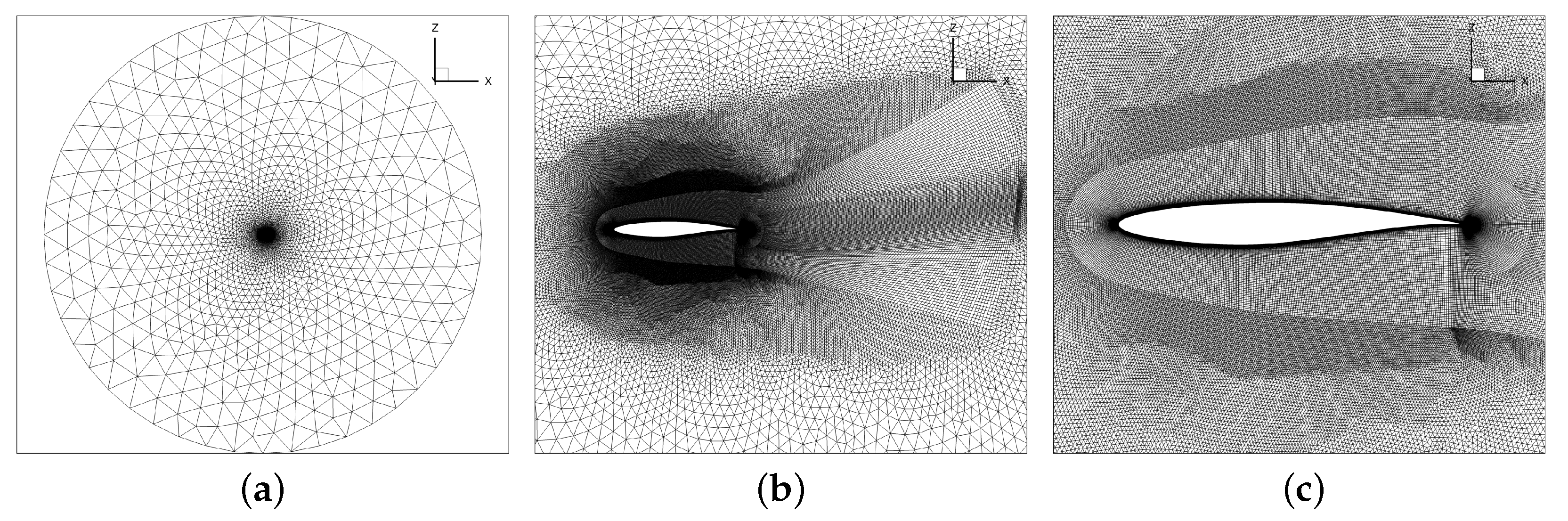
The results are presented for a CFD mesh with about 240.000 nodes, which is depicted in Figure 1. The upper and lower surface of the airfoil are discretized with 300 cells each. The cell size on the main part of the airfoil is about , whereas the leading edge has a finer spacing. It is a hybrid mesh which consists of quadrilateral cells in the vicinity and the wake of the airfoil, see Figure 1b,c, and triangular cells in the remaining parts of the mesh. The farfield extends to a distance of 100 chords in every direction from the airfoil, see Figure 1a. A wall-resolved approach is used and the distances of the first off-body grid nodes satisfy . A grid convergence study is shown in Appendix A.1 and demonstrates the validity of the current mesh.
4. Test Cases and Numerical Settings
Gust encounters are simulated for four different transonic Mach numbers. The Reynolds number of 6.5 Mio is based on the reference chord length of m. Figure 2 depicts the sinusoidal gust velocity around an airfoil, which is used for the excitation of the flow field. The gust length is denoted by and the gust amplitude by . The gust moves over the airfoil with the freestream velocity . So each point in space x is excited by a gust with the same angular frequency , but with a different phase shift . This phase shift depends on a reference coordinate and the actual coordinate x. The vertical gust velocity is defined by
Gust lengths are varied between 2.5 m and 125.5 m, which results in reduced frequencies k of 2.51 down to 0.05 using :
The time step differs slightly for each Mach number, see Table 1, with a non-dimensional time step size of . The time step size is held fixed for all simulated gust lengths at one single Mach number, in order to be able to resolve the same physical effects for each gust length. As a consequence, short gusts are simulated with less time steps per period than long gusts, see Table 2. A convergence study for the time step can be found in Appendix A.2. In any case, the applied CFL number is equal to 50.
Based on the convergence of the mean lift response and the first and second harmonic response, it is decided to define three groups concerning the number of periods computed: shorter gusts are simulated for 20 periods, longer gusts are simulated for 5 periods and all gust lengths in between are simulated for 10 periods, see Table 2. The smallest simulated gust amplitude is as low as m/s in order to guarantee a linear gust response, see Appendix B. Gust amplitudes are increased up to m/s, which is a gust amplitude in the range as demanded by the Certification Specifications. All simulated gust amplitudes are listed in Table 3.
5. Results
5.1. Steady CFD Results
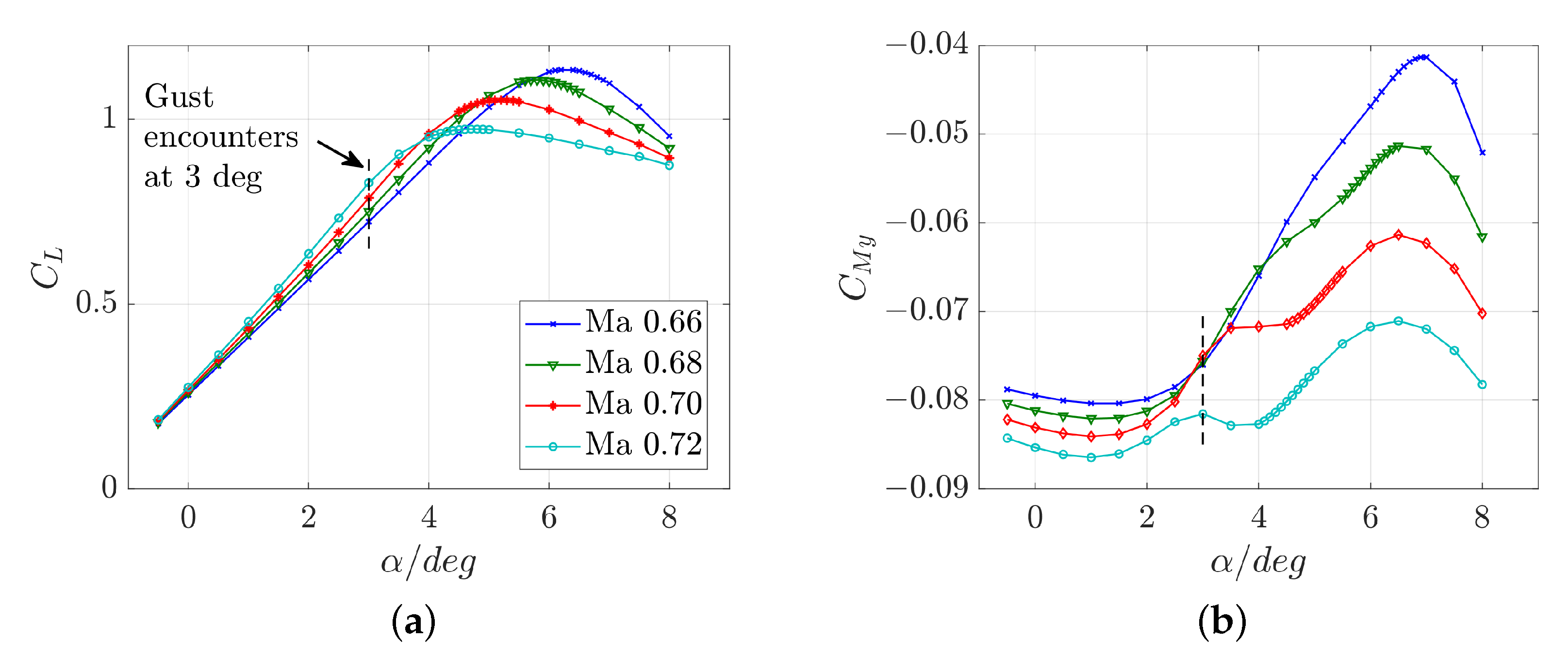
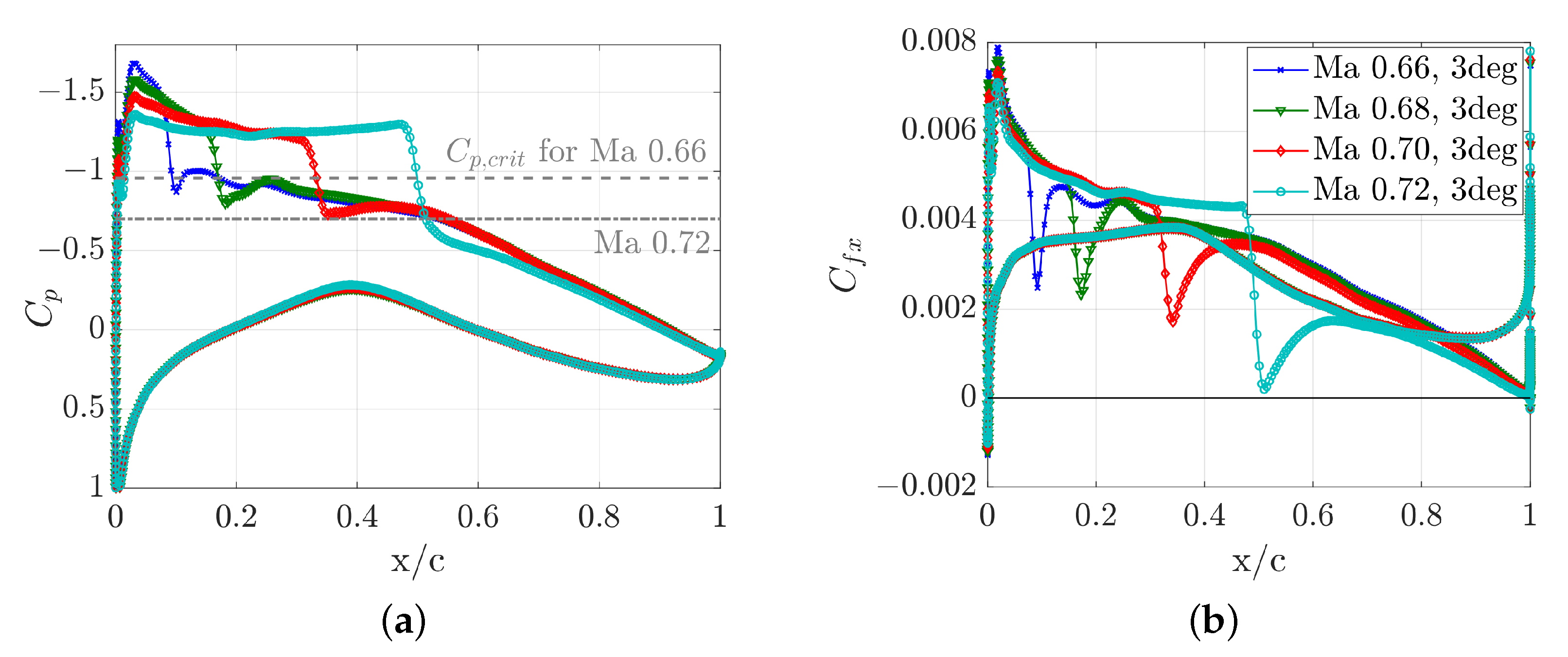
Steady polars are computed for four different Mach numbers: Mach 0.66, 0.68, 0.70 and 0.72 at a Reynolds number of 6.5 Mio. Lift and moment polars are plotted in Figure 3. All lift curves show typical results: with an increase of the Mach number, the maximum lift decreases, but the linear lift curve slope increases. Pitching moment coefficients are referenced to the quarter-chord and show more nonlinear trends than the lift coefficient. The dashed vertical lines mark the steady angle of attack deg, which is used during the gust encounters. Pressure distributions for all Mach numbers reveal transonic conditions, see Figure 4a, and the skin friction coefficients show fully attached flow, see Figure 4b.
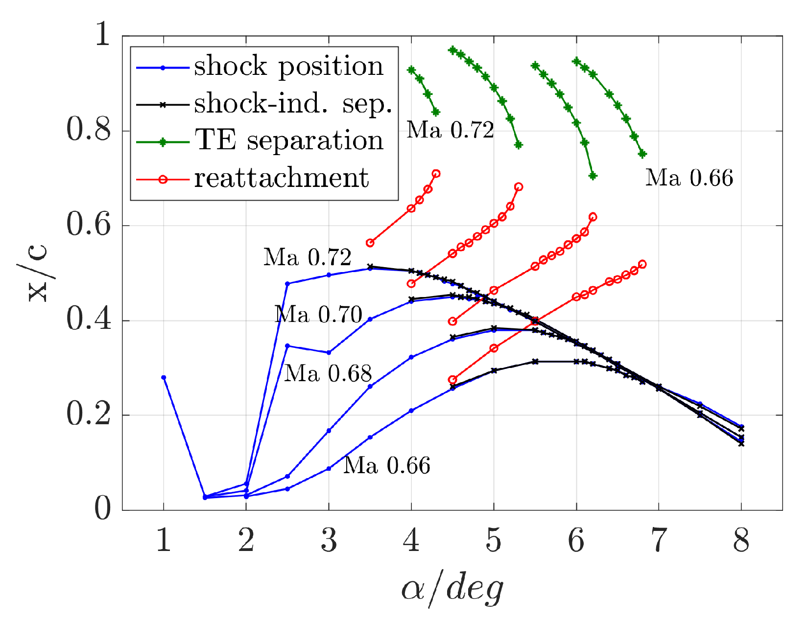
Figure 5 gives an overview about separation and reattachment behavior for this airfoil at the different Mach numbers. Within this work, a shock is detected, if the pressure coefficient is lower than the isentropic critical pressure value , i.e., the local Mach number is higher than 1.0. Then, the x-position of the maximum pressure gradient is defined to be the shock position. Separation occurs if the x-component of the skin friction vector is lower than zero. The qualitative trends of the shock motion and separation are independent from the Mach number: with increasing angle of attack, the shock moves downstream. Until at some condition, shock-induced separation sets in and a separation bubble is formed. Shortly after that angle of attack, the shock reaches its maximum steady position and starts moving upstream, the so-called inverse shock motion sets in. In this specific setting, trailing edge (TE) separation starts at an angle of attack which roughly corresponds to the shock position furthest downstream. This specific fact is just a coincidence and cannot be generalized, as the onset of trailing edge separation is very sensitive to the numerical settings, such as the CFD mesh and turbulence model. At some higher angle of attack, the separation bubble at the shock foot and the trailing edge separation merge and the flow behind the shock starts to be fully separated. Inverse shock motion continues up to the maximum simulated angle of attack. There is a rather large difference in the shock position for the different Mach numbers during the regular shock motion, whereas shock positions during inverse shock motion seem to be almost independent of the Mach number, and more depending on the steady angle of attack. For lower Mach numbers, the transition from fully attached to fully separated flow happens more gradual, i.e., over a wider range of angles of attack, than for higher Mach numbers. Note that the maximum lift coefficient occurs when the shock-induced separation has set in already, but before the flow is fully separated, compare with Figure 3a.
5.2. Unsteady Nonlinear Aerodynamic Responses
5.2.1. Definition of Variables
All gust computations are initiated based on the converged steady-state solutions shown in the previous section. The unsteady lift increment is defined by
where which corresponds to the steady lift coefficient.
For an evaluation of the system behavior, an amplitude-dependent frequency response function (FRF) of the lift, , can be defined using a discrete fourier transform (DFT) such that
The complex-valued Fourier-coefficients of the lift are denoted by for the respective harmonic n, where the highest harmonic N is limited by the steps per period (SPP) for each frequency . The Fourier-coefficient of the first harmonic gust-induced angle of attack is denoted by . Due to the purely sinusoidal excitation, the input signal consists of only one harmonic. Note that only the very last period of each of the computed time signals is used for the DFT.
As it is shown in Appendix B, the responses for the lowest gust amplitude of m/s can be regarded as approximately linear and therefore the computed first harmonic of the FRF can be taken as linear reference value
The incremental linear maximum lift value then results in
The same definitions hold for the pitching moment.
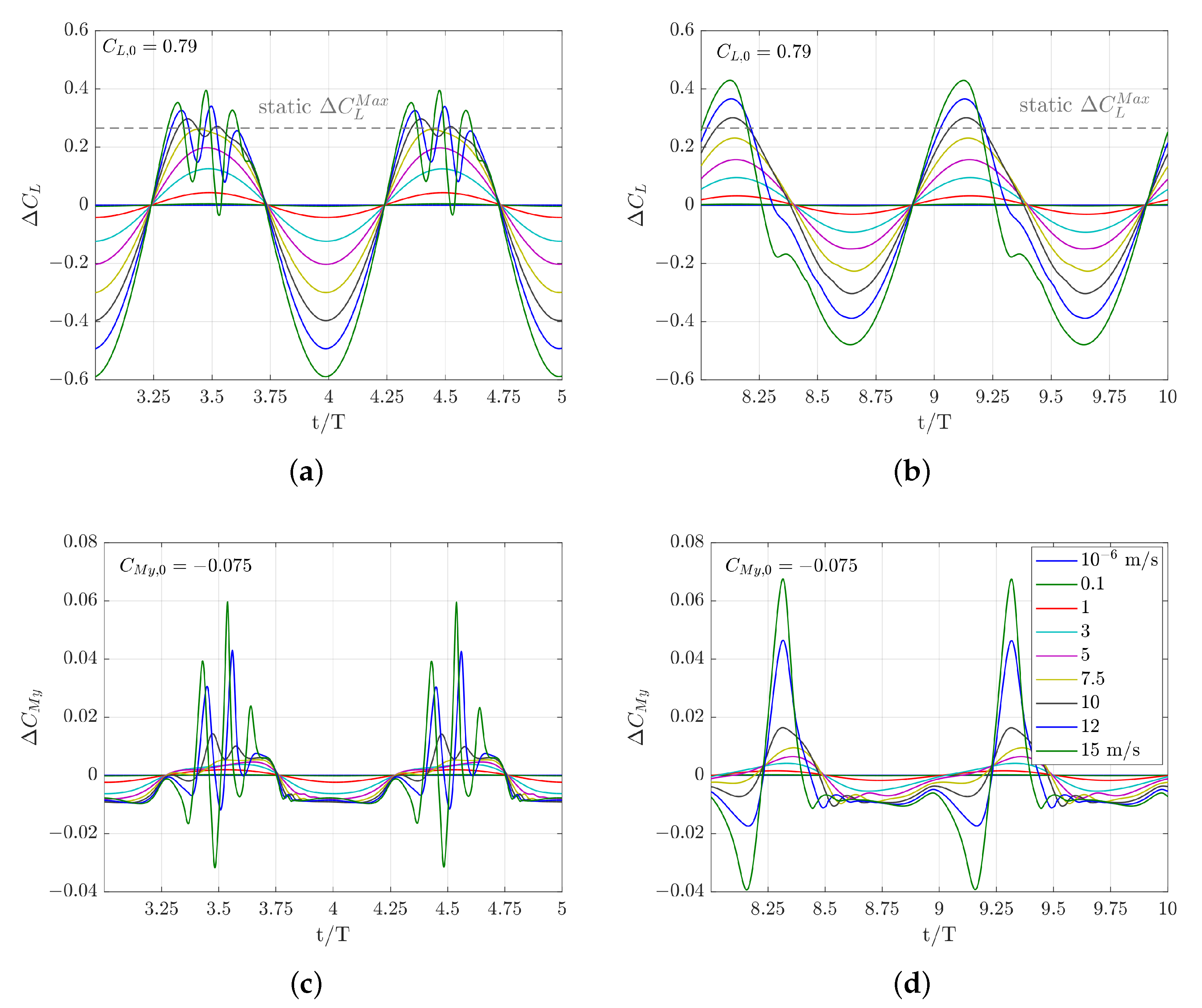
5.2.2. Time-Domain Representation
Exemplarily, Figure 6 shows lift and moment coefficients as a function of time for two different gust lengths and the various amplitudes. The responses to both gust lengths are differently affected by the amplitude nonlinearities, compare Figure 6a,b. They have in common, that an increase in the gust amplitude leads to growing nonlinearities and generally, the pitching moment coefficient is more affected by the large amplitudes. A nonlinear response leads to an earlier breakdown of the lift compared to the linear counterparts. For both gust lengths, first visible deviations from linearity are noticeable at about m/s.
The amplitude effects can be attributed to unsteady flow separation, which occurs similarly in subsonic, dynamic stall-type flows [38]. Some details of the flow field are shown in Section 5.2.6.
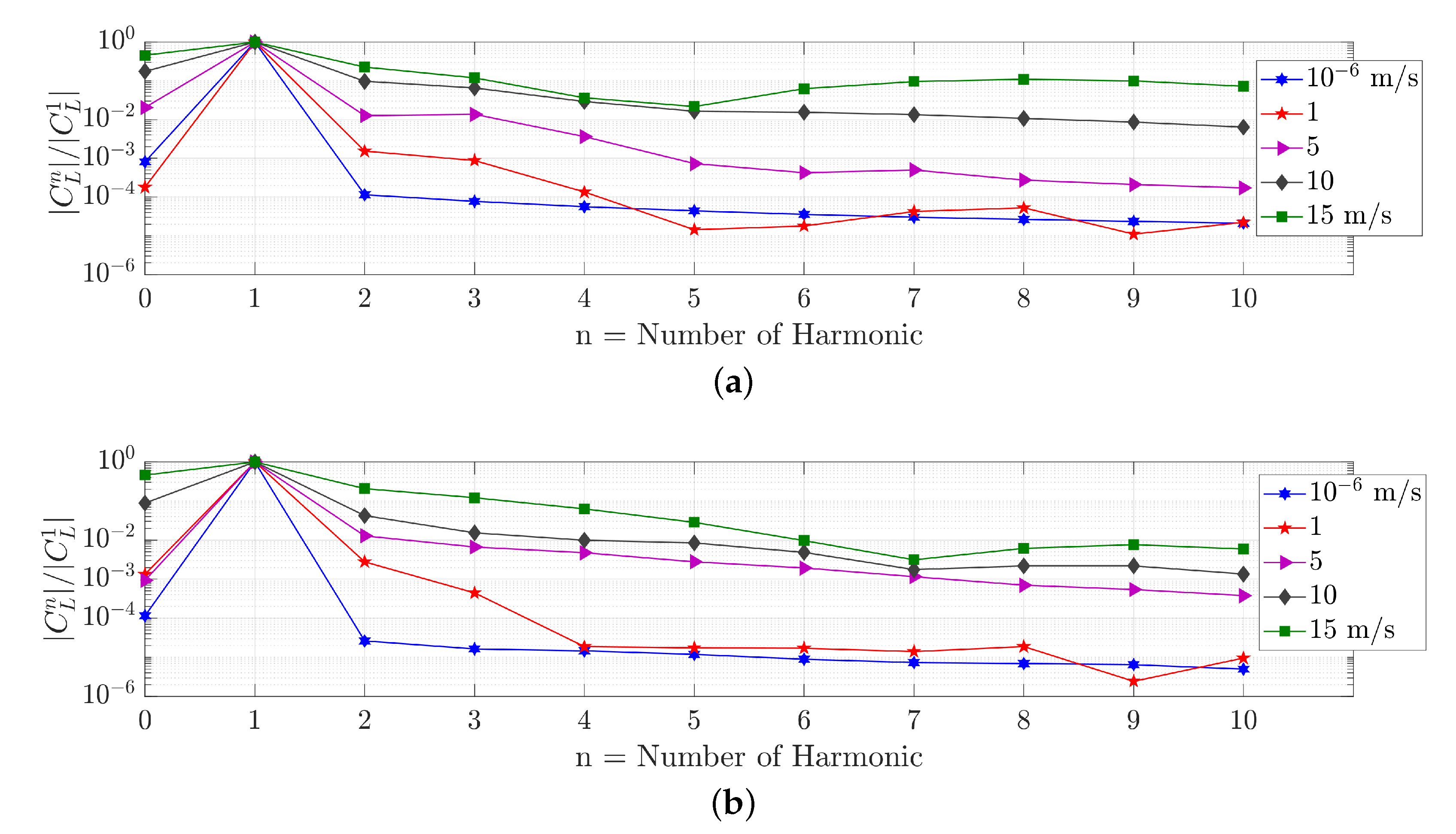
5.2.3. Frequency Content
Especially for the longer gust, higher harmonics are present in the high-amplitude responses, which lead to several peaks in the lift and moment curves. Figure 7 illustrates the distribution of the frequency content for the two gust lengths and 5 amplitudes each. For the definition of the frequency content the reader is referred to Equation (6). Larger gust amplitudes trigger higher harmonic content than smaller gust amplitudes. For the long gust with m/s, even the 10th harmonic is only one order of magnitude lower than the first harmonic. This large number of significant harmonics explains the multiple local maxima in the lift response shown in Figure 6a. For the shorter gust with m/s, the 10th harmonic is at around compared to the first harmonic. In a study by Iovnovich [39] a threshold value for the higher harmonics of is defined to mark the limit between linear and nonlinear responses, while it is admitted that this is a quite arbitrary value. For the cases treated here, a limit for the first 10 harmonics of would mean that the gust amplitude needs to be lower than m/s.
The curves for the harmonics do not decrease monotonically. This is an important fact to notice when reduced-order methods are applied such as the harmonic balance method [15,40]. The shift of the mean value also needs to be taken into account, which is plotted as 0th harmonic in Figure 7. Note that its values do not increase monotonically with increasing excitation amplitude.
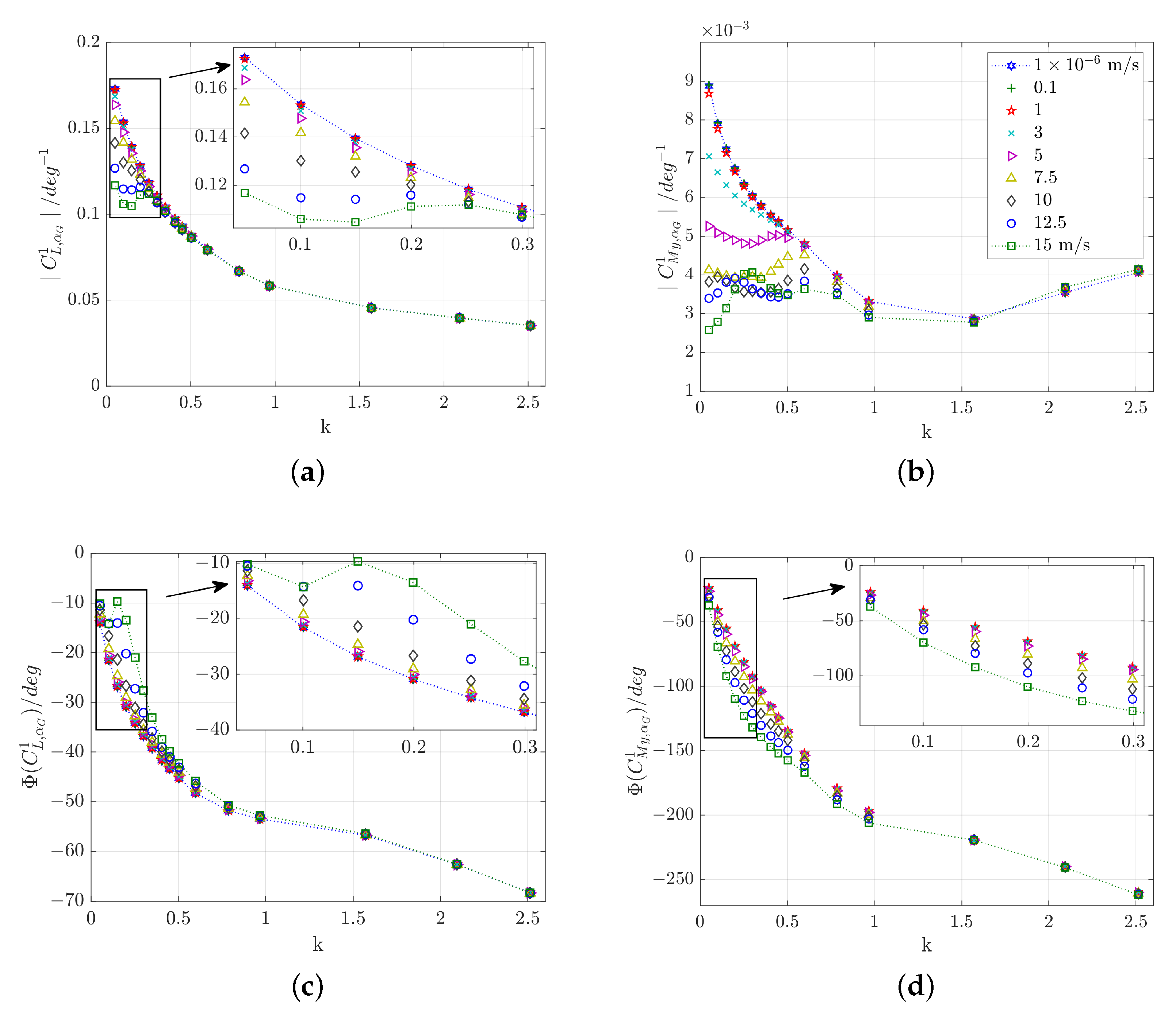
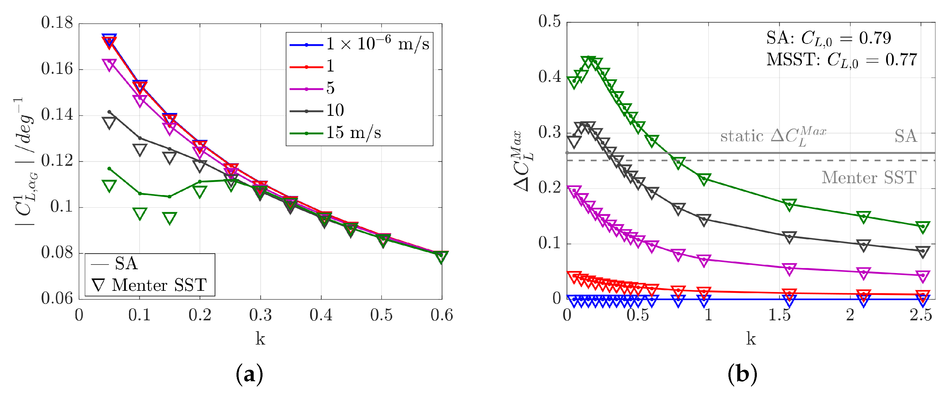
Figure 8 shows the complex first harmonic of lift and moment coefficients for all simulated gust encounters. Both, maximum and minimum gust amplitudes are marked by dotted lines for better identification. As already discussed in the previous section: large amplitudes lead to deviations from the linear response (dotted blue curve) especially for low frequencies. The results in Figure 8 and Figure 9 reveal that nonlinear responses can result in lower or higher first harmonics compared to the linear reference values. This holds for the lift as well as for the pitching moment, though the latter is not shown here. Large amplitudes affect the frequency response functions up to a certain ’limiting frequency’. This limiting frequency strongly depends on the variable studied. There is not only a difference between lift and moment, but also between magnitude and phase. For the gust test cases computed here, the limiting frequencies vary between and , compare Figure 8a–d.
Figure 9 shows the variations for the first harmonic of the lift FRF that result from a change of the inflow Mach number. The maximum gust amplitude of m/s has only little effect on the values for Mach 0.66, whereas at Mach 0.72, gust amplitudes of even 1 m/s deviate from the linear results. This emphasizes the significant effect of the steady-state conditions onto the unsteady results, which are also mentioned in [19]. Moreover, the sudden change of the trend for the larger amplitudes at Mach 0.72 and might be a hint to an involvement of different concurrent unsteady effects. This ’kink’ can be observed with increasing intensity for all four Mach numbers.
Though the computed FRFs result out of gust excitations, qualitatively similar trends can be expected for e.g., a pitching excitation. When the responses are compared for the same excitation amplitude, gust responses are milder than those for a pitching motion [20]. The reason is that gusts do not excite the complete airfoil at the same time, but they are moving over the chord of the airfoil gradually.
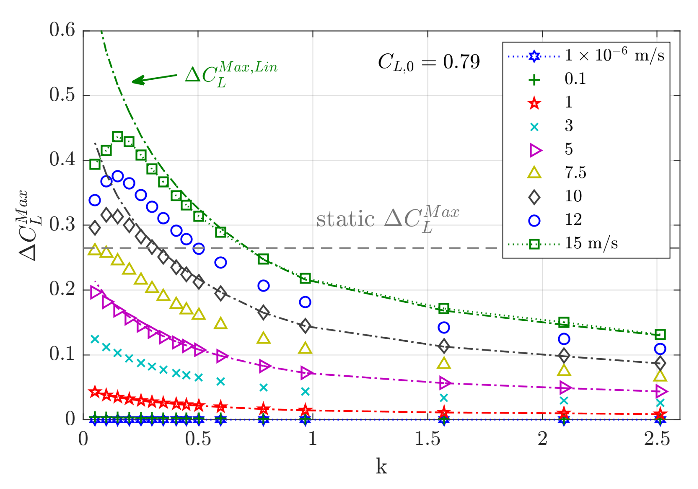
5.2.4. Maximum Lift Coefficient
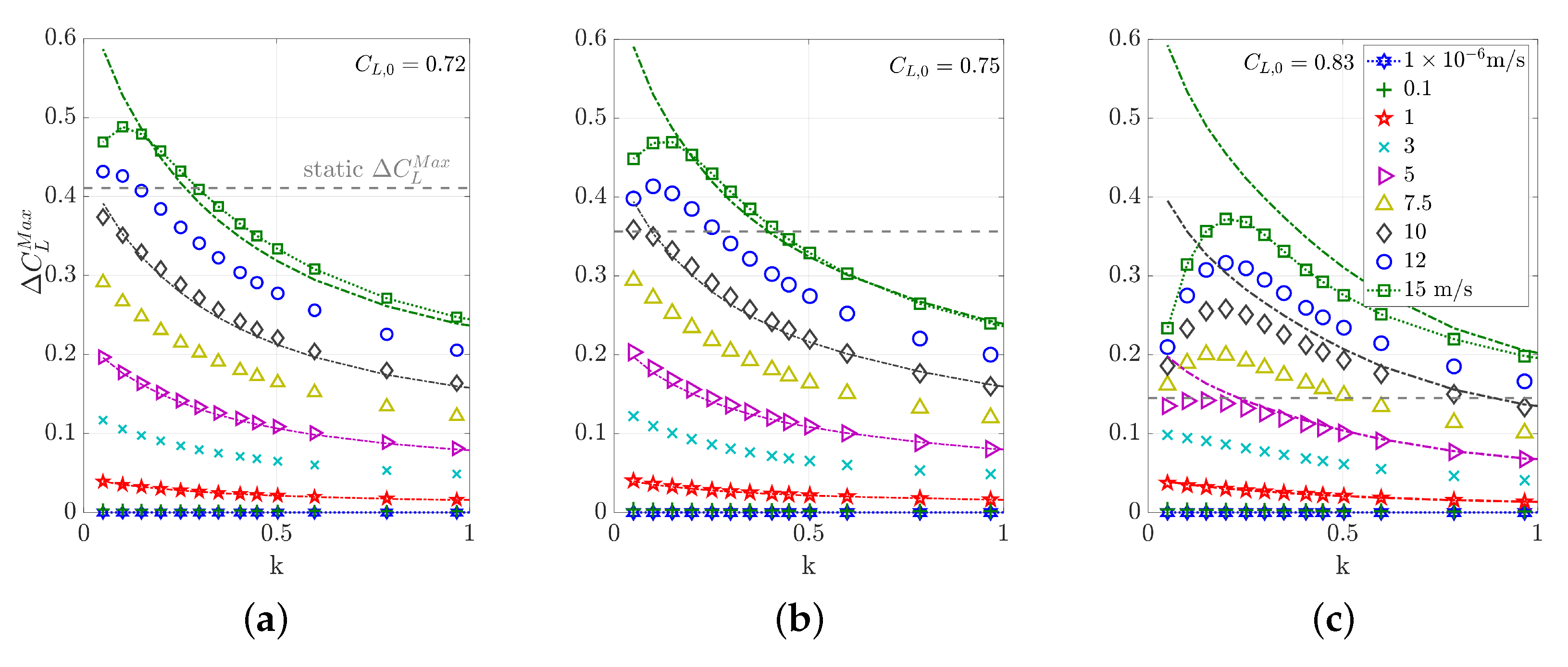
The maximum lift is a relevant value for the loads assessment of an aircraft. Figure 10 summarizes the incremental maximum unsteady lift for all computed gust encounters. Responses to smaller gust amplitudes show a monotonic behavior with increasing frequency, which is a hint for the linearity of the responses. Large amplitudes deviate from the linear results in the range of small frequencies but are almost on-spot for the higher frequencies. Comparing each of the nonlinearly computed maximum lift with its linear reference values (dash-dotted lines), it is noted that first visible deviations occur at m/s. These first deviations occur at lift values that are lower than the static maximum lift. The monotonic trend of the curves is lost when the static maximum lift is overshot for one of the frequencies. With increasing excitation amplitude, the maximum lift moves to higher frequencies. For the cases computed here, there is no saturation found in the maximum lift, but increasing the amplitude leads to higher and higher maximum values. For reduced frequencies higher than 0.7, deviations between linear and nonlinear are not visible anymore. By coincidence, the intersection of each with the static maximum lift value seems to mark the onset of the nonlinear responding range of frequencies at Mach 0.70. This fact is contradicted when looking at the results for the different Mach numbers, see Figure 11. Though all responses which result in a dynamic overshoot deviate from the linear response, it is not the other way round: Maximum lift values that are lower than the static maximum value can also be the result from a nonlinear response. Note that a reduction of the Mach number to Mach 0.66 and Mach 0.68 seems to trigger an overestimation of the nonlinearly computed results compared to the linear ones, whereas an increase of the Mach number to Mach 0.72 seems to facilitate the opposite.
The term ‘dynamic overshoot’ is often used in the context of helicopter dynamic stall [38] in subsonic flows and describes a dynamic exceeding of static maximum loads. Related physical mechanisms are discussed in detail in Ericsson and Reding [41]: dynamic effects lead to a more stable boundary layer and so the onset of flow separation is delayed. In consequence, higher dynamic loads than static loads can occur. The existence of dynamic overshoots in transonic flow, however, is not well investigated and one of the early dynamic stall publications is even questioning their existence [42]. An evidence of transonic dynamic overshoots can be found in [23] for a clean wing configuration under gust excitation and can also be confirmed by the findings in this study. Mainly low excitation frequencies and large amplitudes lead to an overshoot of the static maximum value, independently of the Mach number, see Figure 10 and Figure 11. For Mach 0.72, excitations up to lead to dynamic overshoots, whereas for Mach 0.66, they occur only up to .
5.2.5. Unsteady Shock Motion
One of the prominent features of transonic airfoil flow is the occurence of recompression shocks, which can be detected using the pressure values on the surface of the airfoil, as described in Section 5.1. The surface solutions from the current simulations are stored for 48 samples each period only, and so the shock motion curves are less smooth than e.g., the curves for lift and moment coefficients, compare with Figure 6.
Trends for the unsteady shock motion are shown in Figure 12 for two different gust lengths and various amplitudes. The maximum shock position per excitation period moves further downstream with increasing excitation amplitude. However, a certain saturation of the shock position seems to be reached slightly downstream of the steady maximum position.
Deviations from the sinusoidal shock motion start to show off as early as m/s. This is significantly earlier than it is the case for lift and moment values, see Section 5.2.2. During one period of excitation, the shock starts to vanish for the first time at m/s for m and at m/s for m. The shock motion in upstream direction from the steady-state shock position is much larger than the shock motion in downstream direction.
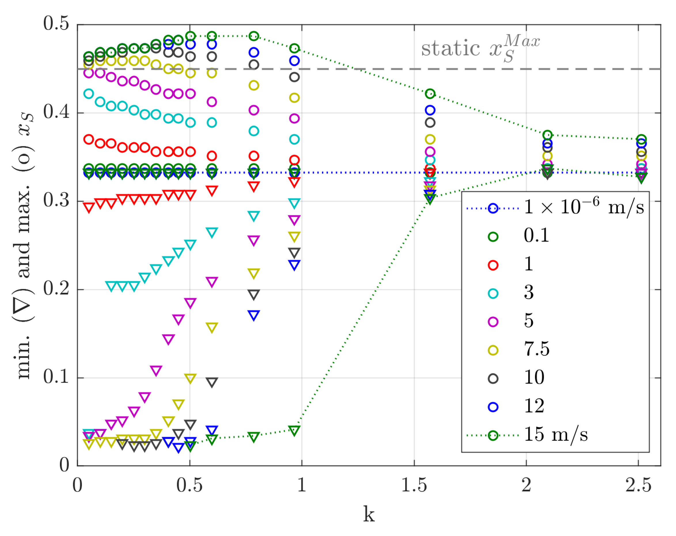
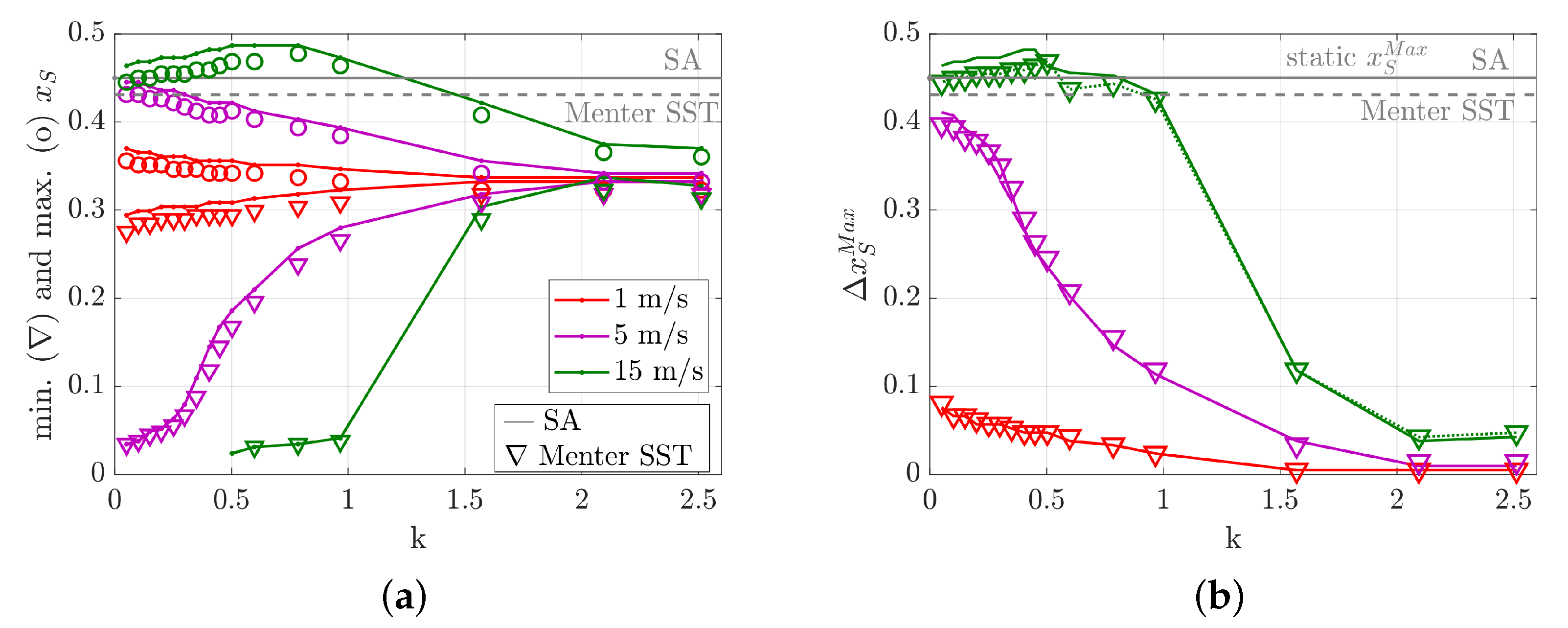
Figure 13 summarizes maximum and minimum x-coordinates for the location of the shock for all excitations at Mach 0.70. The previously mentioned saturation in the maximum downstream shock position occurs up to reduced frequencies of about 0.5. There seems to be a certain mechanism in the flow field which prevents the shock from a further downstream motion. In general, maximum and minimum shock positions show a significant frequency-dependence. Whereas the shock travels by almost 50% over the airfoil chord at lower frequencies, the total shock motion is less than 10% for reduced frequencies as high as 2.0. The shock vanishes partly during one period for lower frequencies and amplitudes larger than 10 m/s.
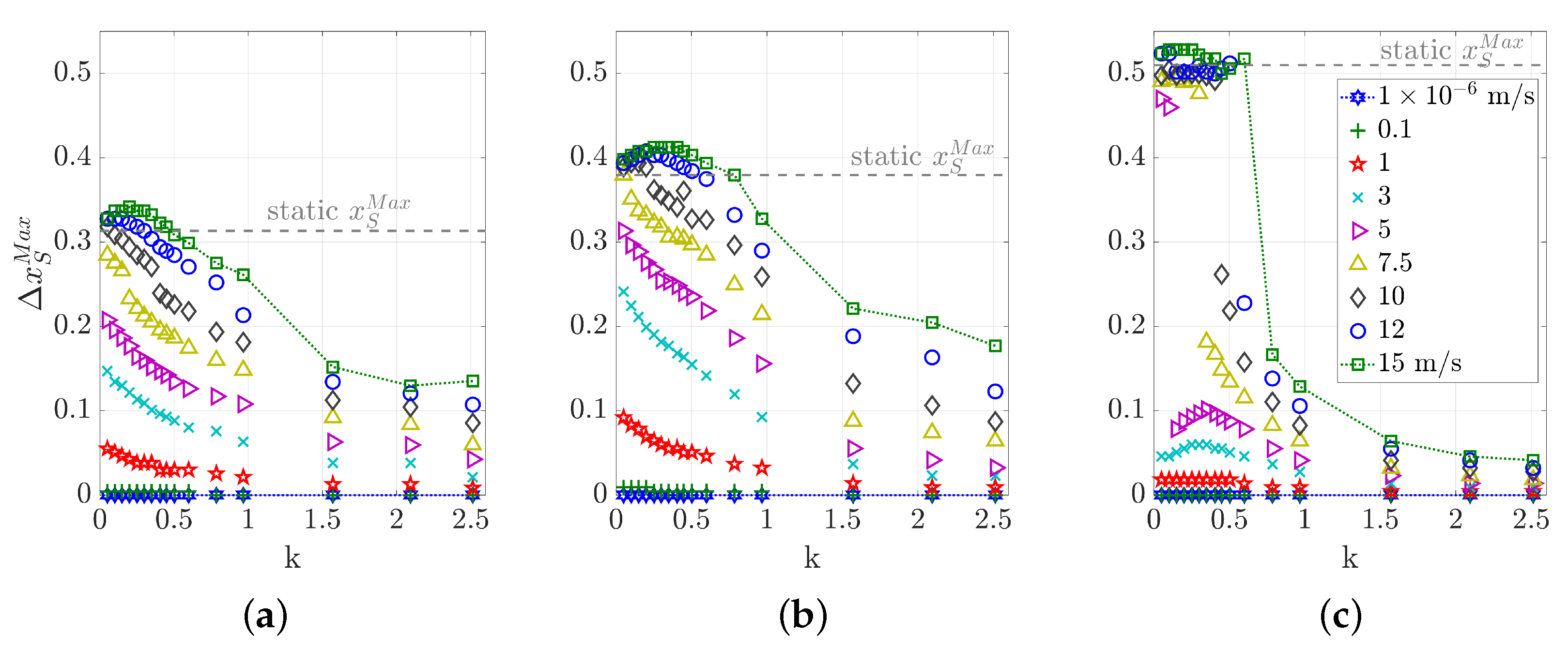
Differences between the shock motion at lower and higher frequencies increase with increasing Mach number, see Figure 14. The maximum shock motion is defined by
For Mach 0.66 and Mach 0.68, trends with respect to the frequency are relatively smooth. For Mach 0.72, the maximum shock motion is as large as 50% of the airfoil chord for reduced frequencies up to 0.6 and rapidly decreases down to 16% for a reduced frequency of 0.7. The saturation in the shock motion that is observed for Mach 0.70 is also found in the data for the other Mach numbers. The static maximum shock position for each Mach number seems to be a good indicator at least for the range of occuring maximum shock motion. However, its exact value is overshot in any case by a few percent.
5.2.6. Examples of Instantaneous Flow Fields
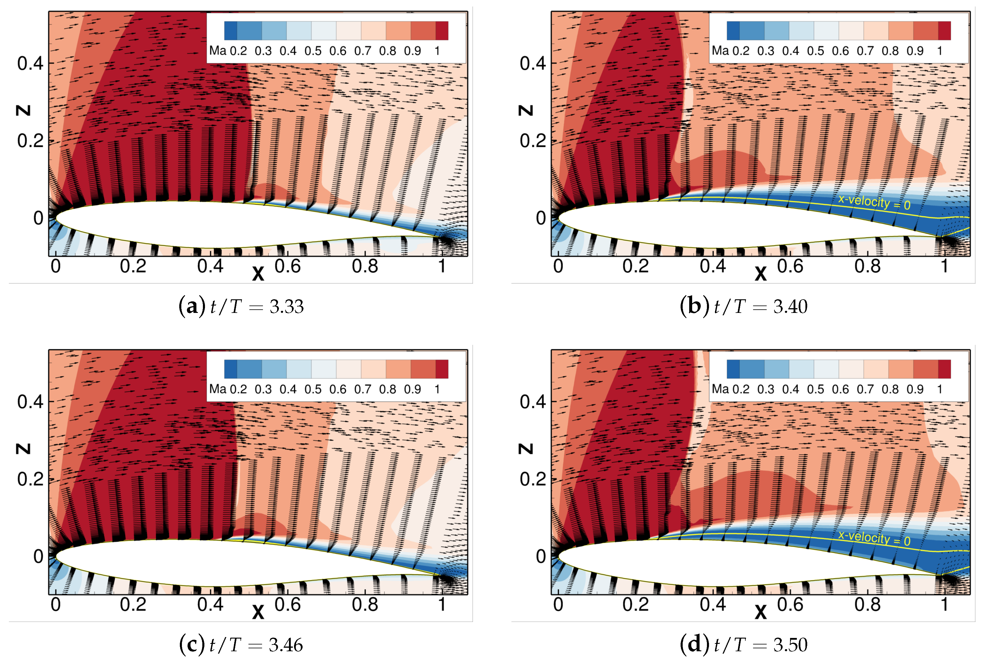
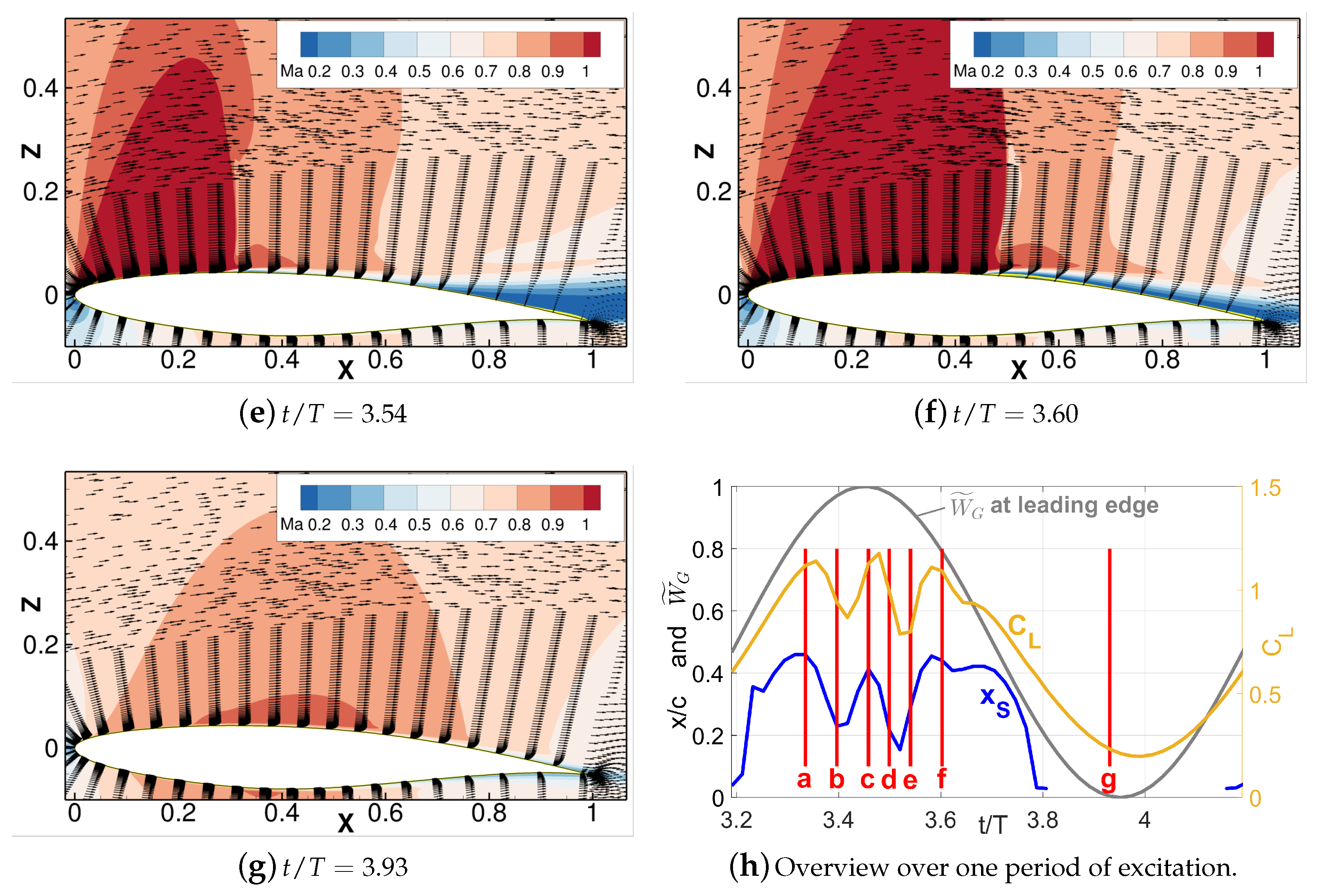
An impression of the flow field for the test case at Mach 0.7 and deg with m and m/s is given in Figure 15. For this long gust, the real time for one period of oscillations amounts to s. Some time histories and the locations of the snapshots (a)–(g) are presented in Figure 15h.
Supersonic regions which extend to almost 50% of the airfoil chord can be observed in snapshots (a)–(f). This is in agreement with the identified shock position shown in Figure 15h. For this specific case, lift and shock motion show three local maxima during one period of oscillation each. Note that the lift curve has a slight lag with respect to the shock motion curve. The snapshot couples (a)–(b) and (c)–(d) reveal a similar dynamic behavior for the first two maxima: just before the peaks, a large supersonic region and a separation bubble about mid-chord of the airfoil are found, see snapshots (a) and (c). The supersonic region then grows further, i.e., the shock moves downstream, until at some point the shock eventually starts to move upstream together with an enlarging region of reversed flow, see snapshots (b) and (d). After snapshot (d), the flow attaches again shortly before snapshot (e) is reached. The third peak in the curves comes without such a big region of reversed flow and is probably limited by the now decreasing edge of the gust velocity. With the decrease of the excitation velocity down to m/s the flow reaches a purely subsonic state, see snapshot (g), which explains the interrupted shock motion curve in Figure 15h.
Due to the complexity of the phenomena involved, further details of the flow fields and related physical effects are planned to be published in a separate paper. Further work will also include an analysis of other test cases computed.
5.2.7. Influence of the Turbulence Model
In order to judge the influence of the turbulence model on the results, some of the gust encounters are re-computed using the two-equation turbulence model Menter SST [33]. The impact of the different modeling on the global response variables is displayed in Figure 16.
Most importantly, none of the previously described trend changes when changing the turbulence model. There are, however, slight differences between the quantitative values of the different models. The first harmonic response is more affected than the maximum lift coefficient, where the results of both models are almost identical. The first harmonic computed with Menter SST is lower than the counterpart computed with the SA model. The deviations in the steady maximum lift coefficient are significantly larger than the differences in the unsteady results. Generally, the deviations nearly vanish for small amplitudes or high frequencies.
The influence of the turbulence model is larger when local variables are assessed, see Figure 17. The SA model predicts all shock positions further downstream than Menter SST, see Figure 17a, which is observed in several publications [35,37,43]. The agreement between the models is improved for the maximum shock motion, see Figure 17b.
5.3. Possible Indicators for the Assessment of Nonlinear Responses
5.3.1. Definition of Variables
Often, the linear response to a specific excitation is not known a priori. It is hard to tell if (and how much) a computed response deviates from the linear reference though this knowledge would be helpful in, e.g., loads or aeroelastic analyses. Therefore, this section examines if the harmonic distortion of the lift, , or the maximum shock motion during one period of excitation, , can be correlated with the extent of nonlinearity of a response.
The following definitions are used for the variables and can similarly be applied to the pitching moment coefficient: The harmonic distortion of the lift response, , is defined as
Values between and are considered in the analysis of the results.
The deviation from the first harmonic of the linear lift response , or in shorter form ’harmonic deviation’ is calculated by
In order to assess the deviation of the computed maximum lift value from the linear lift maximum, , the relative maximum lift is defined using the following equation
5.3.2. Harmonic Distortion
The harmonic distortion weights the amount of higher harmonics with respect to the first harmonic of the response, see Equation (10). It is a common variable in signal analysis to measure the extent of nonlinearity of a response [44,45]. Figure 18 depicts the harmonic distortion for lift and moment coefficients at Mach 0.70 for four different gust amplitudes. Additionally, different numbers of harmonics are considered for the highest gust amplitude, m/s: . For the lift coefficient, 10 harmonics are relevant to represent the harmonic content, whereas even 20 harmonics are necessary for the moment coefficient. These values specifically apply to for this test case. The number of relevant harmonics decreases with increasing frequency. The harmonic distortion for the moment coefficient is significantly higher than the distortion for the lift coefficient, which matches the observations from the previous sections. For low-amplitude excitations, the values generally decrease down to at least single-digit values, see Appendix B.
If a response to a monofrequent excitation is given, the harmonic distortion can be computed to give an impression of the amount of higher harmonics present. The curves in Figure 19 reveal that there is no distinct correlation between the harmonic distortion and the harmonic deviation of the lift. In other words: the amount of harmonic distortion does not express how far off a response is in respect to the actual linear first harmonic at the same reduced frequency. Figure 19a shows that both variables are generally in the same order of magnitudes, but a harmonic distortion of e.g., 10% can correspond to either (for 15 m/s) or to (for 10 m/s). With increasing excitation amplitude, the harmonic distortion tends to larger values compared to the harmonic deviation, i.e., the curves are located more on the right side of the diagram. Contrary, for the smallest frequency considered here, this trends is the other way round. A general shortcoming of the harmonic distortion coefficient is displayed in Figure 19b, which depicts trends for the different Mach numbers. The coefficient does not predict a direction, since it only sums up the magnitudes of the higher harmonics. So a harmonic deviation of e.g., 10% can correspond to either a reduction of the first harmonic magnitude ( for Mach 0.66) or to an augmentation ( for Mach 0.72).
For the relative maximum lift plotted in Figure 20, similar trends are observed as for the previous figure and the same conclusion can be drawn for .
Summing up, the harmonic distortion does not seem to be well suited to predict deviations neither from the linear first harmonic lift derivative, nor from the linear maximum lift value. A large amount of higher harmonics does not, in general, indicate a large deviation from the linear values.
5.3.3. Maximum Shock Motion
The recompression shock is a salient feature of transonic flow. It is investigated in the following, if the motion of the shock throughout a response period does show any correlation with the previously described nonlinear trends in the global loads. Such a correlation is published by Dowell et al. [19] using computations based on the low-frequency transonic small-disturbance approach. Due to the limitations of the numerical method, only reduced frequencies up to 0.3 and amplitudes up to 1.5deg were computed. It is shown that shock motions larger than 5% indicate a deviation of more than 5% from the linear moment derivative.
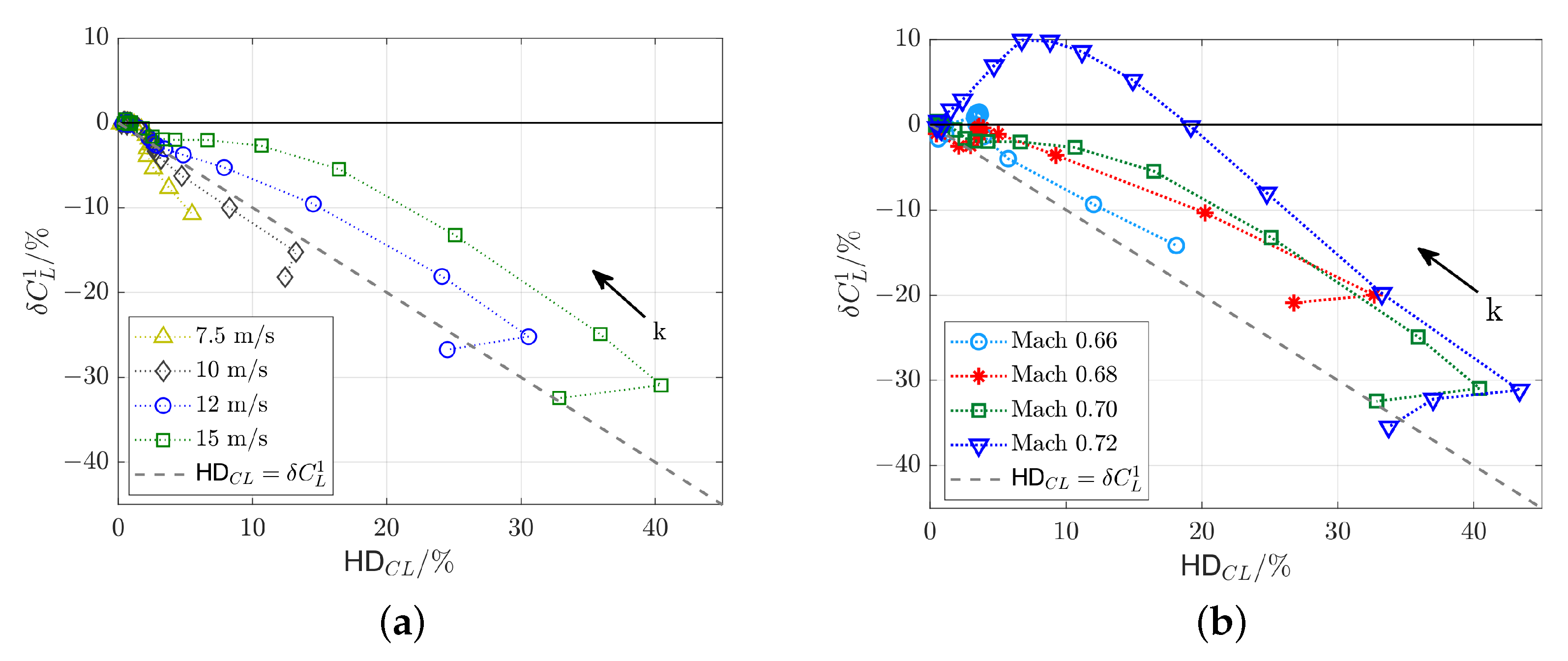
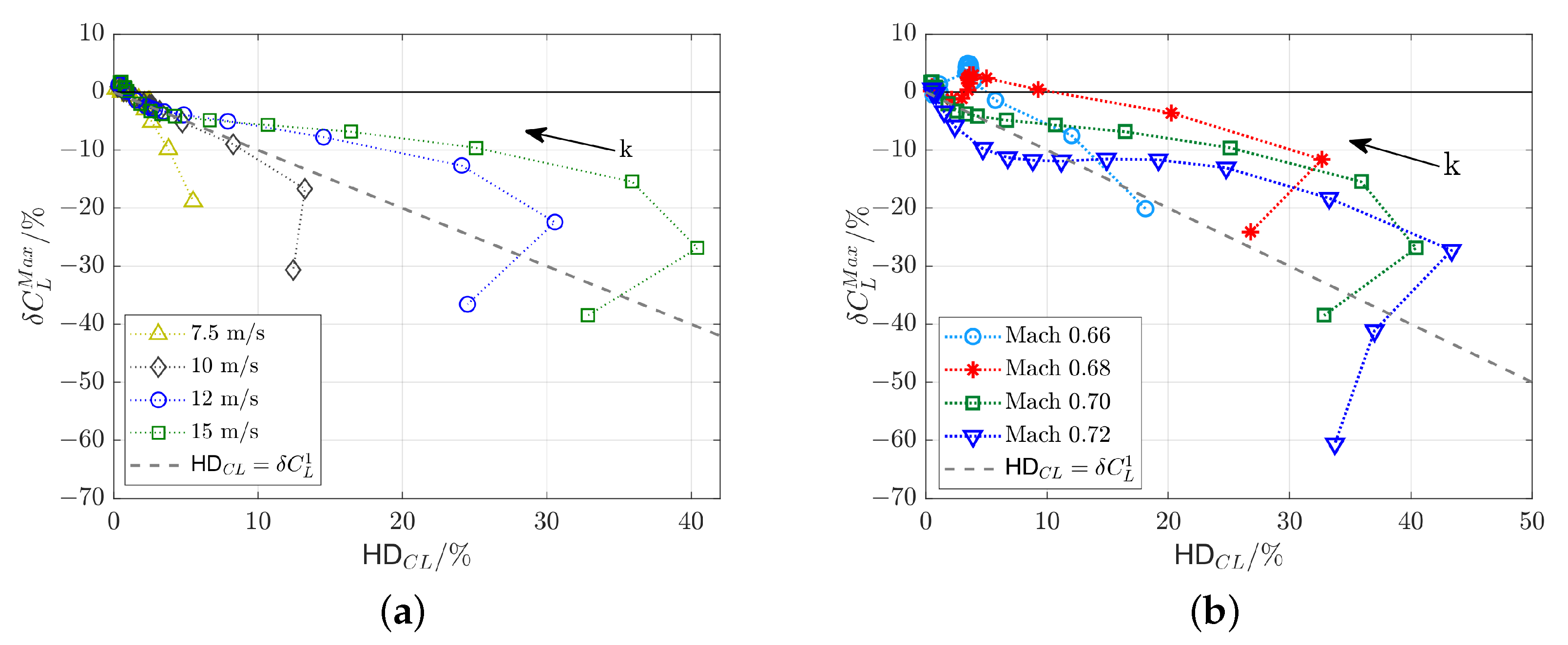
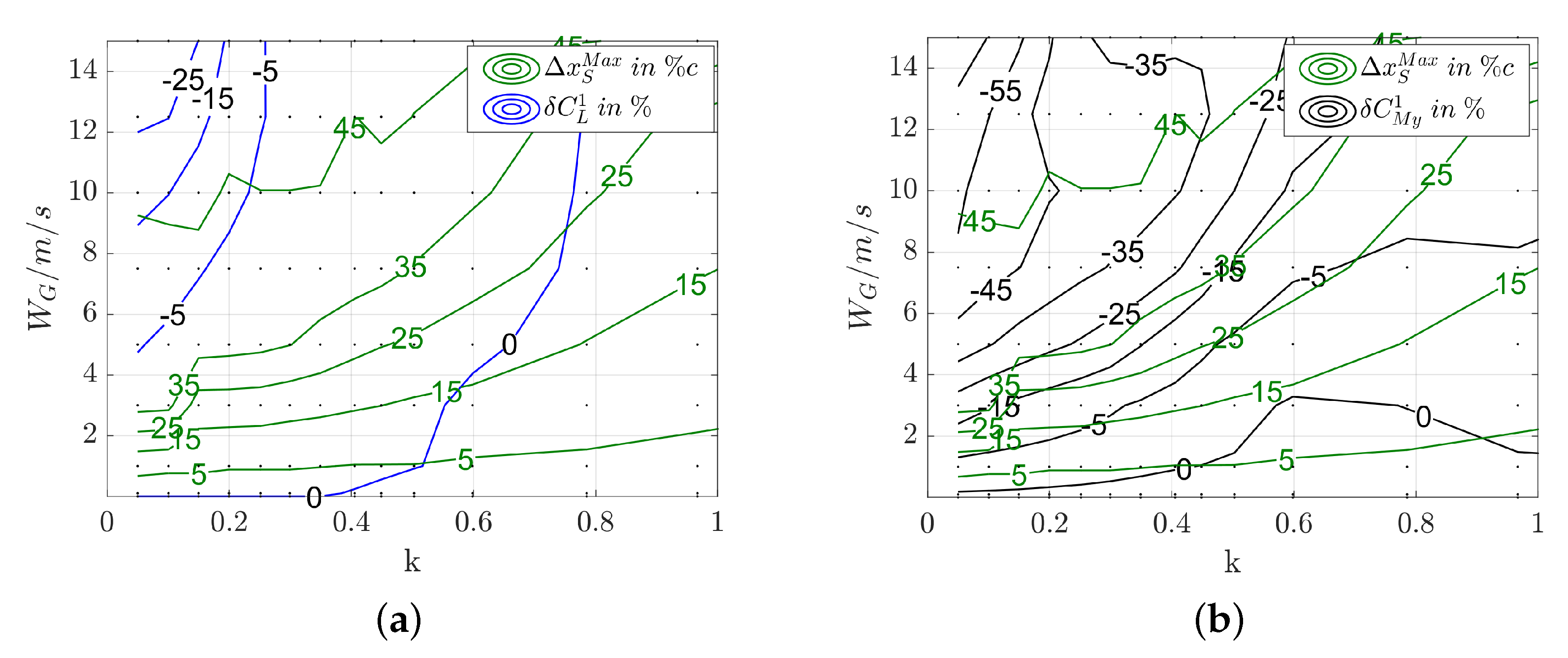
Data from the current study includes a larger range of parameters and is shown in Figure 21 and Figure 22. The contours for the harmonic deviation of lift and moment are plotted against the maximum shock motion in Figure 21. The above-mentioned criterion is met at Mach 0.7: the first harmonic of lift and moment derivatives do not deviate more than 5% from their linear counterparts for a maximum shock motion of 5%. As Dowell et al. [19] already stated, these 5% are a very conservative value: In order to obtain 5% harmonic deviation of the lift, the maximum shock motion can be as large as 35% for the lower frequencies, and even be larger than 45% for reduced frequencies above 0.25. For 5% harmonic deviation of the moment, 5% maximum shock motion are a relatively good indicator at the lowest frequencies, but a maximum shock motion of about 25% can be allowed at higher frequencies. However, the different variables do not correlate very well in general, but show only piecewise similar trends.
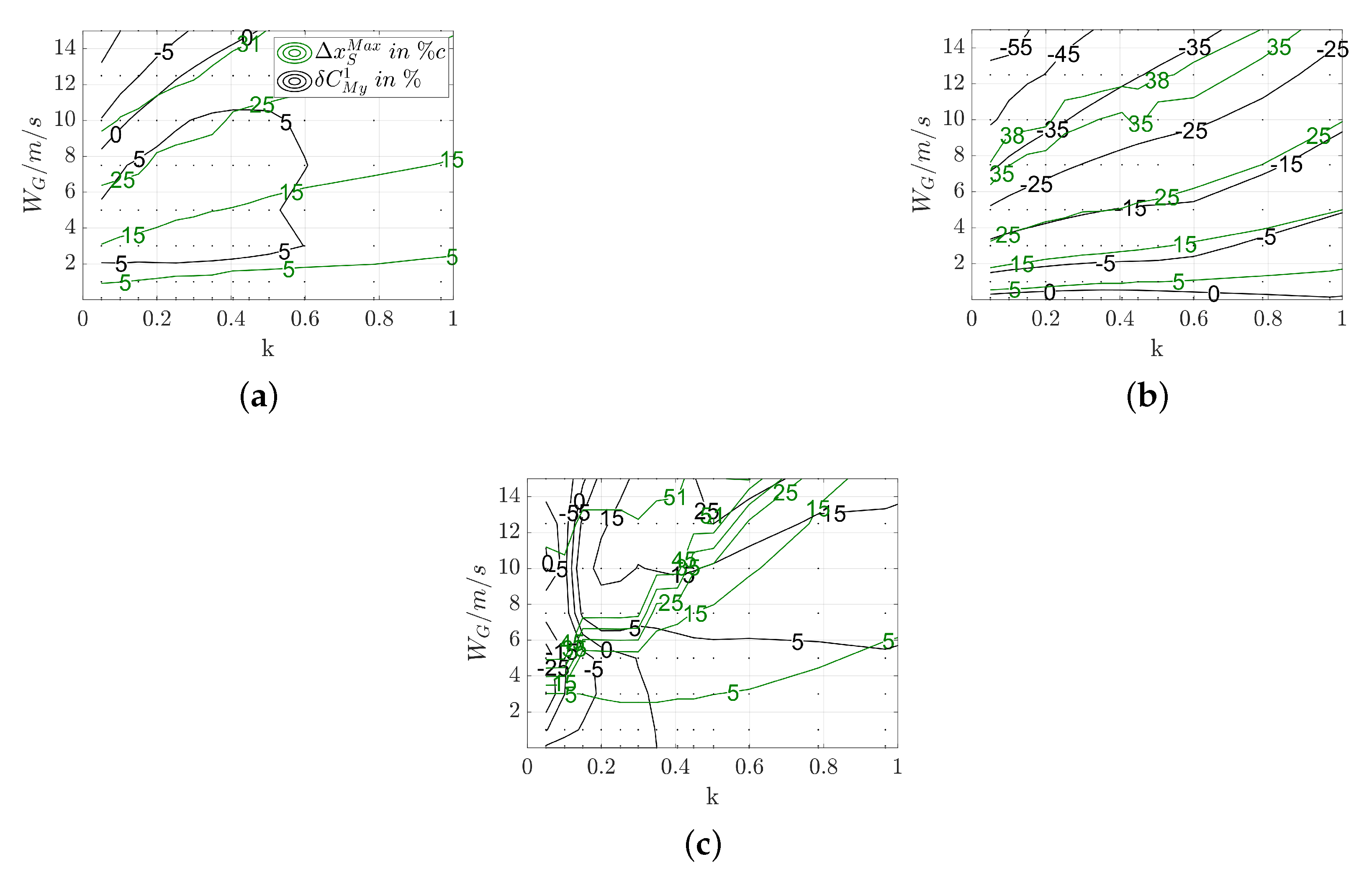
The trends for the different Mach numbers are shown in Figure 22. The contour levels for the shock motion move closer together with increasing Mach number, indicating larger shock motions with increasing Mach number for the same excitation parameters, recall Figure 14. Though the absolute values of the shock motion change with Mach number, their overall trends are very similar, contrary to . The harmonic deviation of the moment changes its overall behavior at every Mach number. Accidentally, the trends for both types of variables are almost congruent at Mach 0.68.
Summing up, the shock motion does not seem to be a reasonable indicator to judge the extent of nonlinearity of the response of an airfoil.
6. Conclusions and Outlook
The physics of unsteady nonlinear transonic flow have been studied relatively little to date and there is a lack especially of fundamental investigations on that topic. In this paper, a parameter study is carried out and it is analyzed with respect to the physics of unsteady nonlinear transonic airfoil flow. Computations are based on the URANS-equations, mainly using the turbulence model Spalart-Allmaras. The flow around the RAE2822 airfoil is excited by sinusoidal gusts with different lengths (i.e., frequencies) and amplitudes. The impact of large-amplitude excitations on global and local parameters is assessed for different inflow Mach numbers.
The results show a clear dependence on the mean steady flow field. Amplitude effects and corresponding nonlinearities grow with increasing Mach number for all variables. Low-frequency results are more affected by the large-amplitude excitations than high-frequency results. Amplitude effects are negligible for the higher frequencies considered, but the limit for this exclusively linearly-responding frequency range strongly depends on the examined variable.
It is shown that the first 10 harmonics of the response need to be considered for an accurate reproduction of the harmonic distortion of the lift coefficient and about 20 harmonics for the moment coefficient. Moreover, it is observed that the first harmonic of lift and moment derivatives are either augmented or reduced in a nonlinear response compared to a linear one. An increase of the derivative is mainly found for the mid-frequency range, a decrease mainly for the lower frequencies.
When nonlinear methods instead of linear methods are used, the predicted maximum lift value is significantly reduced for the lowest frequencies. Depending on the inflow Mach number, nonlinear values can exceed the linear values at higher frequencies. Lower Mach numbers seem to facilitate these overestimates. Additionally, dynamic overshoots of the maximum static lift in transonic flow are found, as well.
The trend of the unsteady shock motion is affected stronger by amplitude effects than the trends of lift and moment coefficients. A saturation of the maximum downstream shock position is observed at lower frequencies for all Mach numbers considered. The maximum steady shock position does not provide an exact threshold for this maximum unsteady shock position, but it can serve as an estimate for that value. For lower frequencies, the maximum shock motion increases with increasing Mach number, but no distinct trend can be found for higher frequencies.
Examplary snapshots of the flow field reveal an interplay of attached and reversed flow as a reason for observed peaks that occur in the lift coefficient. However, a deeper analysis of the phenomena involved remains an aspect of future work.
All of the above-mentioned trends are insensitive with respect to the turbulence model, numerical mesh and the applied time step size. Lastly, neither the variable ’harmonic distortion’ nor the variable ’maximum motion of the recompression shock’ seem to be a reasonable indicator for observed deviations from the linear responses.
Summing up, initially described trends from the literature for three-dimensional aero-elastically coupled configurations can be reproduced using this geometrically simple and purely aerodynamic system. The current two-dimensional setup seems to be suitable for further studies concerning amplitude-nonlinearities without losing the connection to more complex configurations.
The present parameter study shows the variety of results that needs to be covered by newly-developed methods. Depending on the mean steady flow field and the excitation frequency, different trends have to be included. This complicates the development of physics-based reduced-order models that are accurate and computationally fast at the same time. Against this background, the current numerical results can specifically be used to provide reference test cases for the development of unsteady nonlinear ROMs, since a variety of flow conditions and physical effects is included. However, having in mind that mainly the range of lower frequencies is affected by the large-amplitude excitations, nonlinear ROMs would only need to be set up for that specific range. Cheaper time-linearized RANS-based methods could be used for predictions at higher frequencies.
In the future, the current results can be additionally exploited with regard to its unsteady (shock-induced) separation behavior. Similarities and differences to the better known subsonic dynamic stall can be discussed. Analyses of different mode shapes for the excitation and different airfoil geometries can help to ensure the independence of the presented results from this specific application. Finally, it should be emphasized that, to the author’s knowledge, no experimental data is available that can be used for the analysis of unsteady nonlinear response problems in transonic flow and the community is encouraged to publish related data.
Funding
This work was funded by the German Aerospace Center (DLR) in the cross-corridor research project SimBaCon (Simulation Based Certification). There is no external funding involved.
Institutional Review Board Statement
Not applicable.
Informed Consent Statement
Not applicable.
Data Availability Statement
The data presented in this study are available on request from the corresponding author.
Acknowledgments
The author would like to thank Jens Nitzsche from DLR Institute of Aeroelasticity for providing the meshes.
Conflicts of Interest
The author declares no conflict of interest.
Abbreviations
The following abbreviations are used in this manuscript:
| CFD | Computational Fluid Dynamics |
| DFT | Discrete Fourier Transform |
| DLM | Doublet-Lattice Method |
| FRF | Frequency Response Function |
| LFD | Linear Frequency-Domain |
| RANS | Reynolds-Averaged Navier-Stokes |
| ROM | Reduced-Order Model |
| SA | Spalart-Allmaras |
| SST | Shear-Stress Transport |
| TE | Trailing Edge |
| URANS | Unsteady Reynolds-Averaged Navier-Stokes |
Appendix A. Numerical Sensitivities
Appendix A.1. Grid Sensitivity Study
In order to check the spatial convergence, some of the results are reproduced using a significantly finer mesh with a total of about 980.000 nodes and 700 cells on upper and lower surface each. This mesh is denoted as ’fine’ in the following, whereas the mesh used throughout the main part of the paper is denoted as ”medium”, see Section 3. Additionally a ’very fine’ mesh is tested, with about 2.9 million nodes in total and 1350 cells on upper and lower surface each.
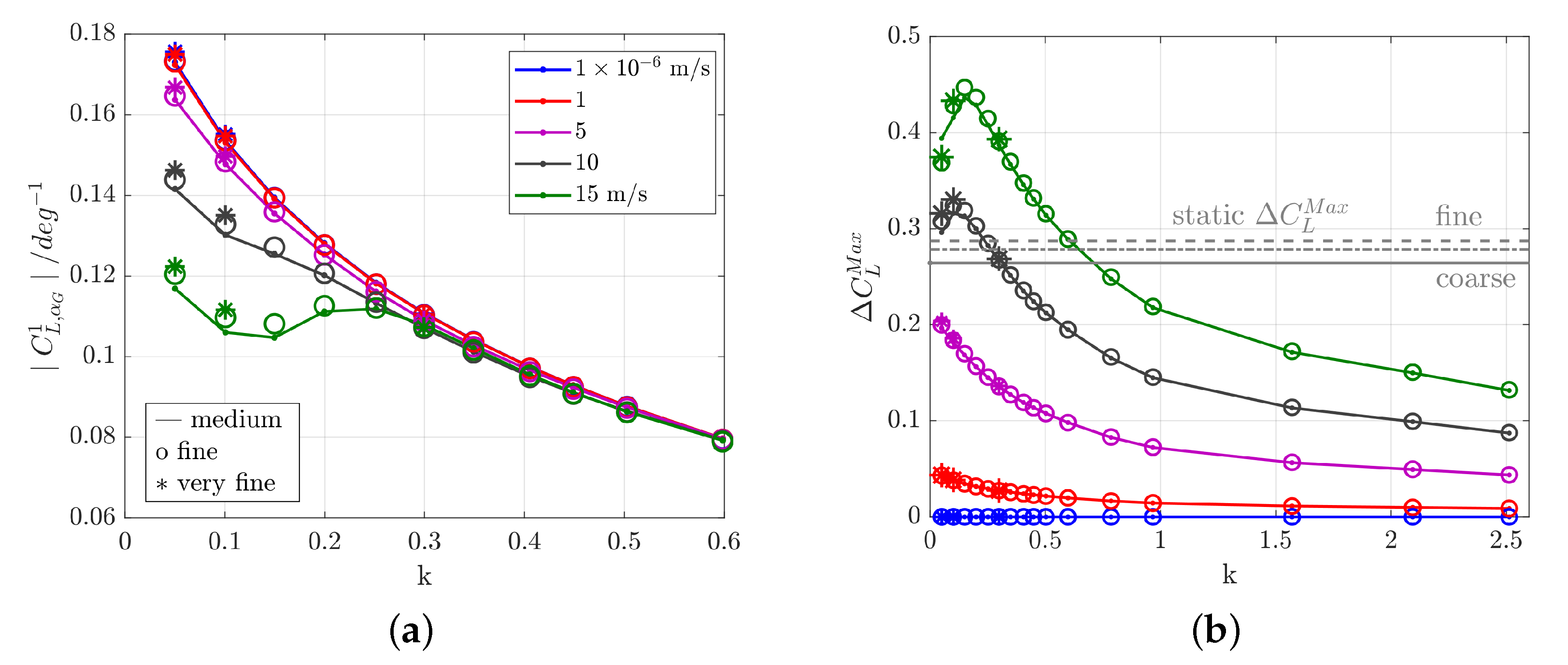
The results for the different meshes are presented in Figure A1. It is noted that the full parameter space is computed for the fine mesh, but only three reduced frequencies are computed for the very fine mesh, due to computational cost. The findings for the mesh convergence study are similar to the ones for the turbulence model study in Section 5.2.7. Overall trends do not change when using the finer meshes and the first harmonic is more influenced by the mesh than the maximum lift coefficient. The two finer meshes shift the values for the magnitude of the first harmonic up to slightly higher values and also predict a slightly higher maximum lift. Due to the very similar results on all three grids, the medium grid is chosen for all computations shown in the main part of the paper.
Figure A1.
Comparison of three CFD meshes at Mach 0.70. (a) First harmonic of the lift FRF, (b) Maximum lift.
Figure A1.
Comparison of three CFD meshes at Mach 0.70. (a) First harmonic of the lift FRF, (b) Maximum lift.

Appendix A.2. Time Step Study
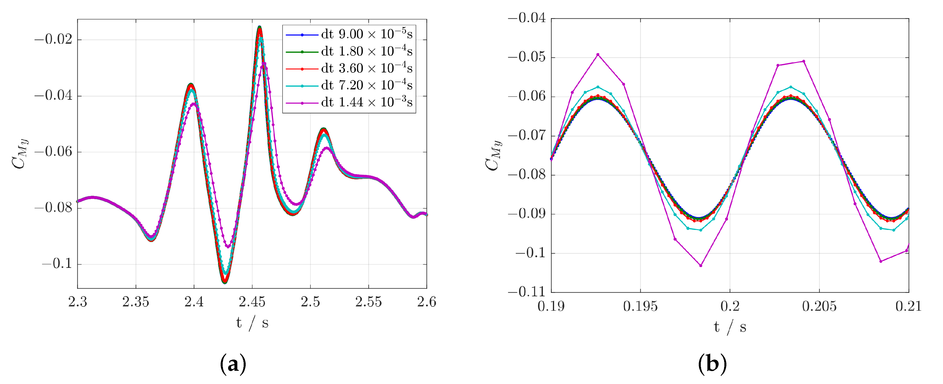
Five different time step sizes are used to compute responses to the lowest and the highest frequency considered, each for the maximum gust amplitude. The results for the pitching moment coefficient are compared in Figure A2. Time step sizes of are tested.
Though the results for both gust lengths show an influence of the time step size, the shorter gust results are more severely affected. For time steps smaller than the results are converged. So for the computations at Mach 0.70 in the main part of the paper, a time step size of s is chosen, see Section 4.
Figure A2.
Comparison of different time step sizes at Mach 0.70. (a) m (k = 0.05), (b) m (k = 2.5).

Appendix B. Verification of Linearity for Low-Amplitude Results
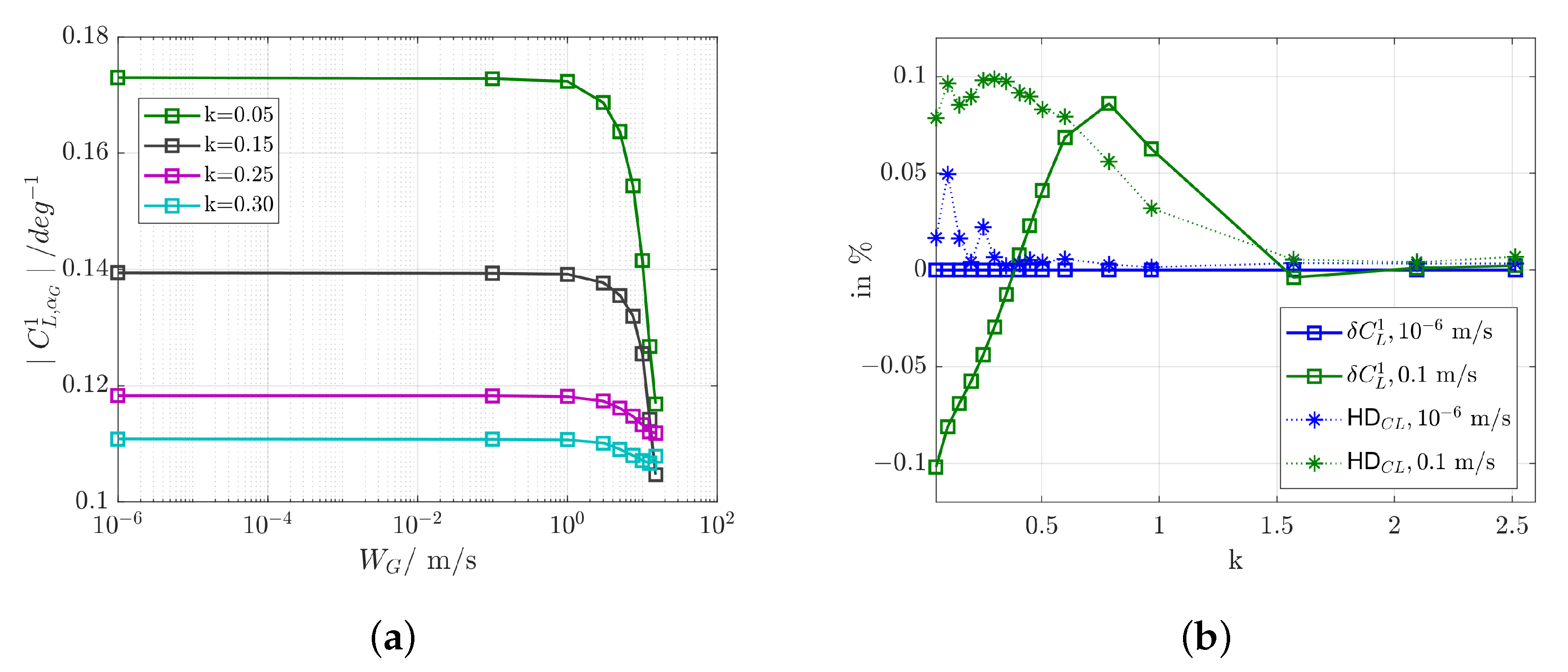
It is stated above, that the results for the lowest excitation amplitude can be taken as linear reference values, which is verified by the data in Figure A3: The first harmonic response of the lift draws a horizontal line between the results at m/s and m/s, see Figure A3a. That shows that the response is independent of the excitation amplitude and therefore corresponds to the definition of a linear system. The same derivative values for the first harmonic could be computed using a RANS-based linear frequency-domain (LFD) approach such as the TAU-LFD solver [46], see e.g., [47] for a detailed comparison.
For a verification of the correct calculation of the variable ’harmonic deviation’, Figure A3b shows its trend for m/s with respect to the reduced frequency. As required by its definition, the harmonic deviation results in zero values for all excitation frequencies. In contrast, the values for m/s differ from zero, but are still on a very low level. Recall from Figure 19, that the maximum gust amplitude results in values in the order of .
As an additional piece of background information, also the harmonic distortion values of the lift are shown for the two lowest excitation amplitudes. Apart from a few outlier, the harmonic distortion is very close to zero for m/s and has only a bit higher values for m/s.
Figure A3.
Verification of linearity for low-amplitude results at Mach 0.70. (a) First harmonic of the lift, (b) Harmonic deviation and and harmonic distortion of the lift for the two lowest excitation amplitudes.
Figure A3.
Verification of linearity for low-amplitude results at Mach 0.70. (a) First harmonic of the lift, (b) Harmonic deviation and and harmonic distortion of the lift for the two lowest excitation amplitudes.

References
- Brink-Spalink, J.; Bruns, J.M. Correction of Unsteady Aerodynamic Influence Coefficients using Experimental or CFD Data; IFASD-2001-034. In Proceedings of the International Forum on Aeroelasticity and Structural Dynamics, Madrid, Spain, 5–7 June 2001. [Google Scholar]
- Karpel, M.; Moulin, B.; Chen, P.C. Dynamic Response of Aeroservoelastic Systems to Gust Excitation. J. Aircr. 2005, 42, 1264–1272. [Google Scholar] [CrossRef]
- Weigold, W.; Stickan, B.; Travieso-Alvarez, I.; Kaiser, C.; Teufel, P. Linearized Unsteady CFD for Gust Loads with TAU. In Proceedings of the International Forum on Aeroelasticity and Structural Dynamics, IFASD-2017-187, Como, Italy, 25–28 June 2017. [Google Scholar]
- Albano, E.; Rodden, W.P. A doublet-lattice method for calculating lift distributions on oscillating surfaces in subsonic flows. AIAA J. 1969, 7, 279–285. [Google Scholar] [CrossRef]
- Giesing, J.P.; Kalman, T.P.; Rodden, W.P. Correction Factor Techniques for Improving Aerodynamic Prediction Methods; NACA-CR-144967; Technical Report; McDonnell Douglas Corporation: St. Louis, MA, USA; NASA: Washington, DC, USA, 1976.
- Palacios, R.; Climent, H.; Karlsson, A.; Winzell, B. Assessment of Strategies for Correcting Linear Unsteady Aerodynamics Using CFD or Experimental Results. In Progress in Computational Flow-Structure Interaction; Haase, W., Selmin, V., Eds.; Springer: Berlin/Heidelberg, Germany, 2003; pp. 209–224. [Google Scholar]
- Thormann, R.; Dimitrov, D. Correction of aerodynamic influence matrices for transonic flow. CEAS Aeronaut. J. 2014, 5, 435–446. [Google Scholar] [CrossRef]
- Banavara, N.K.; Dimitrov, D. Prediction of Transonic Flutter Behavior of a Supercritical Airfoil Using Reduced Order Methods. In New Results in Numerical and Experimental Fluid Mechanics IX; Notes on Numerical Fluid Mechanics and Multidisciplinary Design; Springer International Publishing: Berlin/Heidelberg, Germany, 2014; Volume 124, pp. 365–373. [Google Scholar] [CrossRef] [Green Version]
- Quero-Martin, D. An Aeroelastic Reduced Order Model for Dynamic Response Prediction to Gust Encounters. Ph.D. Thesis, Institute of Aeroelasticity, Berlin, Germany, 2017. [Google Scholar] [CrossRef]
- Katzenmeier, L.; Vidy, C.; Breitsamter, C. Correction Technique for Quality Improvement of Doublet Lattice Unsteady Loads by Introducing CFD Small Disturbance Aerodynamics. J. Aeroelasticity Struct. Dyn. 2017, 5, 17–40. [Google Scholar] [CrossRef]
- Bekemeyer, P.; Thormann, R.; Timme, S. Frequency-Domain Gust Response Simulation Using Computational Fluid Dynamics. AIAA J. 2017, 55, 2174–2185. [Google Scholar] [CrossRef]
- Bekemeyer, P.; Ripepi, M.; Heinrich, R.; Görtz, S. Nonlinear Unsteady Reduced-Order Modeling for Gust-Load Predictions. AIAA J. 2019, 57, 1839–1850. [Google Scholar] [CrossRef]
- Halder, R.; Damodaran, M.; Khoo, B.C. Deep Learning Based Reduced Order Model for Airfoil-Gust and Aeroelastic Interaction. AIAA J. 2020, 58, 4304–4321. [Google Scholar] [CrossRef]
- Lucia, D.J.; Beran, P.S.; Silva, W.A. Reduced-order modeling: New approaches for computational physics. Prog. Aerosp. Sci. 2004, 40, 51–117. [Google Scholar] [CrossRef] [Green Version]
- Hall, K.C.; Thomas, J.P.; Clark, W.S. Computation of Unsteady Nonlinear Flows in Cascades Using a Harmonic Balance Technique. AIAA J. 2002, 40, 879–886. [Google Scholar] [CrossRef] [Green Version]
- Leishman, J.G.; Beddoes, T.S. A Generalised Model for Airfoil Unsteady Aerodynamic Behaviour and Dynamic Stall Using the Indicial Method. In Proceedings of the American Helicopter Society (AHS) Annual Forum, New York, NY, USA, 2–5 June 1986. [Google Scholar]
- Reddy, T.S.R.; Kaza, K.R.V. Comparative Study of Some Dynamic Stall Models; Technical Report; NASA: Washington, DC, USA, 1987.
- Goman, M.; Khrabrov, A. State-space representation of aerodynamic characteristics of an aircraft at high angles of attack. J. Aircr. 1994, 31, 1109–1115. [Google Scholar] [CrossRef]
- Dowell, E.H.; Williams, M.H.; Bland, S.R. Linear/Nonlinear Behavior in Unsteady Transonic Aerodynamics. AIAA J. 1983, 21, 38–46. [Google Scholar] [CrossRef]
- Mallik, W.; Raveh, D.E. Kriging-Based Aeroelastic Gust Response Analysis at High Angles of Attack. AIAA J. 2020, 58, 3777–3787. [Google Scholar] [CrossRef]
- Kaiser, C.; Quero, D.; Nitzsche, J. Quantification of Nonlinear Effects in Gust Load Prediction. In Proceedings of the International Forum on Aeroelasticity and Structural Dynamics, Savannah, GA, USA, 10–13 June 2019. [Google Scholar]
- Mallik, W.; Raveh, D.E. Gust Response at High Angles of Attack. AIAA J. 2019, 57, 3250–3260. [Google Scholar] [CrossRef]
- Friedewald, D.; Thormann, R.; Kaiser, C.; Nitzsche, J. Quasi-steady doublet-lattice correction for aerodynamic gust response prediction in attached and separated transonic flow. CEAS Aeronaut. J. 2017, 9, 53–66. [Google Scholar] [CrossRef]
- European Aviation Safety Agency (EASA). Certification Specifications and Acceptable Means of Compliance for Large Aeroplanes CS-25, Amendment 12; Technical Report; European Aviation Safety Agency (EASA): Cologne, Germany, 2012.
- Gerhold, T.; Galle, M.; Friedrich, O.; Evans, J. Calculation of complex three-dimensional configurations employing the DLR-TAU-code. In Proceedings of the 35th Aerospace Sciences Meeting and Exhibit, San Diego, CA, USA, 5–9 January 1997. [Google Scholar] [CrossRef]
- Schwamborn, D.; Gerhold, T.; Heinrich, R. The DLR TAU-Code: Recent Applications in Research and Industry. In Proceedings of the European Conference on Computational Fluid Dynamics (ECCOMAS), Egmond aan Zee, The Netherlands, 5–8 September 2006. [Google Scholar]
- Jameson, A.; Schmidt, W.; Turkel, E. Numerical Solutions of the Euler Equations by the Finite Volume Methods Using Runge Kutta Time Stepping Schemes. In Proceedings of the 14th Fluid and Plasma Dynamics Conference, AIAA 81–1259, Palo Alto, CA, USA, 23–25 June 1981. [Google Scholar] [CrossRef] [Green Version]
- Jameson, A. Time Dependent Calculations using Multigrid, with Applications to Unsteady Flows past Airfoils and Wings. In Proceedings of the 10th Computational Fluid Dynamics Conference, AlAA 91-1596, Honolulu, HI, USA, 24–26 June 1991. [Google Scholar] [CrossRef]
- Heinrich, R. Simulation of Interaction of Aircraft and Gust Using the TAU-Code. In New Results in Numerical and Experimental Fluid Mechanics IX; Notes on Numerical Fluid Mechanics and Multidisciplinary Design; Springer International Publishing: Berlin/Heidelberg, Germany, 2014; Volume 124, pp. 503–511. [Google Scholar] [CrossRef]
- Spalart, P.; Allmaras, S. A One-Equation Turbulence Model for Aerodynamic Flows. In Proceedings of the 30th Aerospace Sciences Meeting and Exhibit, AIAA-92-0439, Reno, NV, USA, 6–9 January 1992. [Google Scholar] [CrossRef]
- Deutsches Zentrum für Luft- und Raumfahrt (DLR). TAU-Code User Guide 2016.1.0; Technical Report; Deutsches Zentrum für Luft- und Raumfahrt (DLR): Braunschweig, Germany, 2016. [Google Scholar]
- Giannelis, N.F.; Vio, G.A.; Levinski, O. A review of recent developments in the understanding of transonic shock buffet. Prog. Aerosp. Sci. 2017, 92, 39–84. [Google Scholar] [CrossRef]
- Menter, F.R. Two-Equation Eddy-Viscosity Turbulence Models for Engineering Applications. AIAA J. 1994, 8, 1598–1605. [Google Scholar] [CrossRef] [Green Version]
- Cook, P.H.; McDonald, M.A.; Firmin, M.C.P. Aerofoil RAE 2822: Pressure Distributions, and Boundary Layer and Wake Measurements; Technical Report AGARD-AR-138, AGARD; North Atlantic Treaty Organization: Brussels, Belgium, 1979. [Google Scholar]
- Bardina, J.E.; Huang, P.G.; Coakley, T.J. Turbulence Modeling Validation, Testing and Development; NASA Technical Memorandum 110446; Ames Research Center: Moffett Field, CA, USA, 1997. [Google Scholar]
- Hellström, T.; Davidson, L.; Rizzi, A. Reynolds Stress Transport Modelling of Transonic Flow around the RAE2822 Airfoil. In 32nd Aerospace Sciences Meeting and Exhibit; American Institute of Aeronautics and Astronautics: Reno, NV, USA, 1994. [Google Scholar] [CrossRef]
- Knopp, T. Validation of the Turbulence Models in the DLR TAU Code for Transonic Flows—A Best Practice Guide; Forschungsbericht 2006-01; Institut für Aerodynamik und Strömungsmechanik: Göttingen, Germany, 2006. [Google Scholar]
- McCroskey, W.J.; McAlister, K.W.; Carr, L.W.; Pucci, S.L.; Lambert, O.; Indergrand, R.F. Dynamic Stall on Advanced Airfoil Sections. J. Am. Helicopter Soc. 1981, 26, 40–50. [Google Scholar] [CrossRef]
- Iovnovich, M.; Raveh, D. Transonic Unsteady Aerodynamics in the Vicinity of Shock-Buffet Instability. J. Fluids Struct. 2012, 29, 131–142. [Google Scholar] [CrossRef]
- Thormann, R.; Timme, S. Application of Harmonic Balance Method for Non-linear Gust Responses. In AIAA SciTech Forum; American Institute of Aeronautics and Astronautics: Reston, VA, USA, 2018. [Google Scholar] [CrossRef]
- Ericsson, L.; Reding, J. Dynamic stall overshoot of static airfoil characteristics. In 12th Atmospheric Flight Mechanics Conference; American Institute of Aeronautics and Astronautics: Snowmass, CO, USA, 1985. [Google Scholar] [CrossRef]
- Harper, P.W.; Flanigan, R.E. The Effect of Rate of Change of Angle of Attack in the Maximum Lift of a Small Model; Technical Report NACA Technical Note 2061; NACA TN 2061; NACA: Alabama Birmingham, AL, USA, 1950. [Google Scholar]
- Dimitrov, D. Unsteady aerodynamics of wings with an oscillating flap in transonic flow. In Proceedings of the 8th PEGASUS-AIAA Student Conference, Poitiers, France, 11–13 April 2012. [Google Scholar]
- Shmilovitz, D. On the definition of total harmonic distortion and its effect on measurement interpretation. IEEE Trans. Power Deliv. 2005, 20, 526–528. [Google Scholar] [CrossRef]
- Davis, S.; Malcolm, G. Unsteady Aerodynamics of Conventional and Supercritical Airfoils. In Structures, Structural Dynamics, and Materials and Co-Located Conferences; American Institute of Aeronautics and Astronautics: Reston, VA, USA, 1980. [Google Scholar] [CrossRef]
- Thormann, R.; Widhalm, M. Linear-Frequency-Domain Predictions of Dynamic-Response Data for Viscous Transonic Flows. AIAA J. 2013, 51, 2540–2557. [Google Scholar] [CrossRef]
- Kaiser, C.; Thormann, R.; Dimitrov, D.; Nitzsche, J. Time-Linearized Analysis of Motion-Induced and Gust-Induced Airloads with the DLR TAU Code; Deutscher Luft-und Raumfahrtkongress: Rostock, Germany, 2015. [Google Scholar]
Figure 1.
Hybrid CFD mesh for the RAE2822 airfoil with about 240.000 nodes. (a) Far-field mesh, (b) Quads in the near-field and the wake, (c) Close-up of the near-field mesh.
Figure 1.
Hybrid CFD mesh for the RAE2822 airfoil with about 240.000 nodes. (a) Far-field mesh, (b) Quads in the near-field and the wake, (c) Close-up of the near-field mesh.

Figure 2.
Sketch of a sinusoidal gust that is used for the excitation of the flow.

Figure 3.
Steady polars for the RAE2822 airfoil. (a) Lift, (b) Pitching moment.

Figure 4.
Local coefficients for different Mach numbers at 3 deg. (a) Pressure coefficients, (b) Skin friction coefficients.
Figure 4.
Local coefficients for different Mach numbers at 3 deg. (a) Pressure coefficients, (b) Skin friction coefficients.

Figure 5.
Trends in separation and reattachment for the different Mach numbers.

Figure 6.
Global coefficients for two gust lengths and various amplitudes at Mach 0.70. (a) m (k = 0.05), (b) m (k = 0.20), (c) m (k = 0.05), (d) m (k = 0.20).
Figure 6.
Global coefficients for two gust lengths and various amplitudes at Mach 0.70. (a) m (k = 0.05), (b) m (k = 0.20), (c) m (k = 0.05), (d) m (k = 0.20).

Figure 7.
Normalized frequency content of the lift coefficient. (a) m (k = 0.05), (b) m (k = 0.20).

Figure 8.
First harmonic of lift and moment frequency response functions (FRFs) for all simulated excitations at Mach 0.70. (a) Magnitude of lift first harmonic, (b) Magnitude of moment first harmonic, (c) Phase of lift first harmonic, (d) Phase of moment first harmonic.
Figure 8.
First harmonic of lift and moment frequency response functions (FRFs) for all simulated excitations at Mach 0.70. (a) Magnitude of lift first harmonic, (b) Magnitude of moment first harmonic, (c) Phase of lift first harmonic, (d) Phase of moment first harmonic.

Figure 9.
Magnitude of lift first harmonic. (a) Mach 0.66, (b) Mach 0.68, (c) Mach 0.72.

Figure 10.
Maximum lift during one period of excitation at Mach 0.70, compared to .

Figure 11.
Maximum lift increment during one period of excitation. (a) Mach 0.66, (b) Mach 0.68, (c) Mach 0.72.
Figure 11.
Maximum lift increment during one period of excitation. (a) Mach 0.66, (b) Mach 0.68, (c) Mach 0.72.

Figure 12.
Shock motion for two gust lengths and various amplitudes at Mach 0.70. (a) m (k = 0.05), (b) m (k = 0.20).
Figure 12.
Shock motion for two gust lengths and various amplitudes at Mach 0.70. (a) m (k = 0.05), (b) m (k = 0.20).

Figure 13.
Minimum and maximum x-coordinates for the shock position during one period of excitation at Mach 0.70.
Figure 13.
Minimum and maximum x-coordinates for the shock position during one period of excitation at Mach 0.70.

Figure 14.
Maximum shock motion during one period of excitation. (a) Mach 0.66, (b) Mach 0.68, (c) Mach 0.72.
Figure 14.
Maximum shock motion during one period of excitation. (a) Mach 0.66, (b) Mach 0.68, (c) Mach 0.72.

Figure 15.
(a–g): Snapshots of Mach number contours including velocity vectors. Additionally, the yellow line in the field plots shows the contour for x-velocity = 0. (h): Lift, shock motion and normalized gust velocity during one period of excitation.
Figure 15.
(a–g): Snapshots of Mach number contours including velocity vectors. Additionally, the yellow line in the field plots shows the contour for x-velocity = 0. (h): Lift, shock motion and normalized gust velocity during one period of excitation.


Figure 16.
Global variables in comparison between Spalart-Allmaras (solid lines) and Menter SST (symbols) at Mach 0.70. (a) First harmonic of the lift FRF, (b) Maximum lift.
Figure 16.
Global variables in comparison between Spalart-Allmaras (solid lines) and Menter SST (symbols) at Mach 0.70. (a) First harmonic of the lift FRF, (b) Maximum lift.

Figure 17.
Shock motion in comparison between Spalart-Allmaras (solid lines) and Menter SST (symbols) at Mach 0.70, (a) Minimum and maximum x-coordinates for the shock position, (b) Maximum shock motion during one period of excitation.
Figure 17.
Shock motion in comparison between Spalart-Allmaras (solid lines) and Menter SST (symbols) at Mach 0.70, (a) Minimum and maximum x-coordinates for the shock position, (b) Maximum shock motion during one period of excitation.

Figure 18.
Harmonic distortion for Mach 0.70, (a) (Note: lines for n = 50 and n = 20 coincide with n = 10 and are not displayed), (b) (Note: the line for n = 50 coincides with n = 20 and is not displayed).
Figure 18.
Harmonic distortion for Mach 0.70, (a) (Note: lines for n = 50 and n = 20 coincide with n = 10 and are not displayed), (b) (Note: the line for n = 50 coincides with n = 20 and is not displayed).

Figure 19.
Harmonic deviation as a function of the harmonic distortion of the lift , which is computed using 10 harmonics. (a) Mach 0.70, (b) m/s.
Figure 19.
Harmonic deviation as a function of the harmonic distortion of the lift , which is computed using 10 harmonics. (a) Mach 0.70, (b) m/s.

Figure 20.
Relative maximum lift as a function of the harmonic distortion of the lift , which is computed using 10 harmonics. (a) Mach 0.70, (b) m/s.
Figure 20.
Relative maximum lift as a function of the harmonic distortion of the lift , which is computed using 10 harmonics. (a) Mach 0.70, (b) m/s.

Figure 21.
Harmonic deviation of lift and moment in comparison to the maximum shock motion at Mach 0.70. (grey dots denote the computed test cases). (a) , (b) .
Figure 21.
Harmonic deviation of lift and moment in comparison to the maximum shock motion at Mach 0.70. (grey dots denote the computed test cases). (a) , (b) .

Figure 22.
Harmonic deviation of the moment in comparison to the maximum shock motion. (a) Mach 0.66, (b) Mach 0.68, (c) Mach 0.72.
Figure 22.
Harmonic deviation of the moment in comparison to the maximum shock motion. (a) Mach 0.66, (b) Mach 0.68, (c) Mach 0.72.


Table 1.
Time step size: %c per time step for each Mach number.
| Mach | [m/s] | dt [s] | Inner Iterations |
|---|---|---|---|
| 0.66 | 218.65 | 400 | |
| 0.68 | 225.28 | 400 | |
| 0.70 | 231.90 | 400 | |
| 0.72 | 238.52 | 400 |
Table 2.
Numerical settings for different gust lengths, independent of the Mach number (SPP: steps per period, ndt: total number of time steps).
Table 2.
Numerical settings for different gust lengths, independent of the Mach number (SPP: steps per period, ndt: total number of time steps).
| [ m] | k | SPP | nr. of Periods | ndt |
|---|---|---|---|---|
| 2.5 | 2.51 | 60 | 20 | 1200 |
| ⋮ | ⋮ | ⋮ | ⋮ | ⋮ |
| 18.0 | 0.35 | 432 | 20 | 8640 |
| 21.0 | 0.30 | 504 | 10 | 5040 |
| 25.0 | 0.25 | 600 | 10 | 6000 |
| 31.5 | 0.20 | 756 | 10 | 7560 |
| 42.0 | 0.15 | 1008 | 10 | 10,080 |
| 62.5 | 0.10 | 1500 | 5 | 7500 |
| 125.5 | 0.05 | 3012 | 5 | 15,060 |
Table 3.
Gust velocities and gust-induced angles of attack at Mach 0.70, using .
| [ m/s] | [] |
|---|---|
| 0.1 | 0.025 |
| 1.0 | 0.25 |
| 3.0 | 0.74 |
| 5.0 | 1.24 |
| 7.5 | 1.85 |
| 10.0 | 2.47 |
| 12.5 | 3.09 |
| 15.0 | 3.70 |
Publisher’s Note: MDPI stays neutral with regard to jurisdictional claims in published maps and institutional affiliations. |
© 2020 by the author. Licensee MDPI, Basel, Switzerland. This article is an open access article distributed under the terms and conditions of the Creative Commons Attribution (CC BY) license (http://creativecommons.org/licenses/by/4.0/).
Share and Cite
MDPI and ACS Style
Friedewald, D. Numerical Simulations on Unsteady Nonlinear Transonic Airfoil Flow. Aerospace 2021, 8, 7. https://0-doi-org.brum.beds.ac.uk/10.3390/aerospace8010007
AMA Style
Friedewald D. Numerical Simulations on Unsteady Nonlinear Transonic Airfoil Flow. Aerospace. 2021; 8(1):7. https://0-doi-org.brum.beds.ac.uk/10.3390/aerospace8010007
Chicago/Turabian StyleFriedewald, Diliana. 2021. "Numerical Simulations on Unsteady Nonlinear Transonic Airfoil Flow" Aerospace 8, no. 1: 7. https://0-doi-org.brum.beds.ac.uk/10.3390/aerospace8010007
Note that from the first issue of 2016, this journal uses article numbers instead of page numbers. See further details here.