
Analysis of the Cosmic Ray Effects on Sentinel-1 SAR Satellite Data


1
Remote Sensing and GIS Graduate Program, Institute of Science and Technology, Akdeniz University, Antalya 07058, Turkey
2
Department of Space Science and Technologies, Faculty of Science, Akdeniz University, Antalya 07058, Turkey
*
Author to whom correspondence should be addressed.
Aerospace 2021, 8(3), 62; https://0-doi-org.brum.beds.ac.uk/10.3390/aerospace8030062
Submission received: 7 January 2021
/
Revised: 19 February 2021
/
Accepted: 21 February 2021
/
Published: 3 March 2021
Abstract
:Ionizing radiation sources such as Solar Energetic Particles and Galactic Cosmic Radiation may cause unexpected errors in imaging and communication systems of satellites in the Space environment, as reported in the previous literature. In this study, the temporal variation of the speckle values on Sentinel 1 satellite images were compared with the cosmic ray intensity/count data, to analyze the effects which may occur in the electromagnetic wave signals or electronic system. Sentinel 1 Synthetic Aperture Radar (SAR) images nearby to the cosmic ray stations and acquired between January 2015 and December 2019 were processed. The median values of the differences between speckle filtered and original image were calculated on Google Earth Engine Platform per month. The monthly median “noise” values were compared with the cosmic ray intensity/count data acquired from the stations. Eight selected stations’ data show that there are significant correlations between cosmic ray intensities and the speckle amounts. The Pearson correlation values vary between 0.62 and 0.78 for the relevant stations.
1. Introduction
Cosmic rays are various atomic and subatomic particles that continuously enter the Earth’s atmosphere from the Sun and outside of the Solar System and reach the Earth [1]. They are studied in two groups as primary and secondary cosmic rays. Primary cosmic rays are energetic particles that reach the Earth’s atmosphere and consist of approximately 83% protons, 13% alpha particles, 1% nuclei with atomic number >2 and 3% electrons [2]. As cosmic rays pass through the atmosphere, they interact with atoms and molecules in the atmosphere, thus producing lower energy particles. These particles with lower energy reaching the ground are secondary cosmic rays. Cosmic rays are also divided into three categories: Galactic Cosmic Rays (GCR) coming from outside the solar system; Solar Energetic Particles, which are defined as high-energy particles emitted by Solar Explosions or coronal mass ejections (CMEs); and Extragalactic Cosmic Rays, which flow into the Solar System from beyond the Milky Way galaxy. Cosmic rays have high enough energy to affect the electronic circuit components and optical materials of satellites. They can cause signal attenuation, deterioration of GPS calibration, complete loss of the signal, incorrect operations, equipment damage and thus undesirable effects on communication and image acquisition [3].
For satellites in the space environment, there are many factors that will affect the performance or lifetime of these satellites. Sun or galactic radiation is one among these factors. Due to the high amount of ionizing radiation in the space environment, it is important to examine this radiation for all kinds of space missions [4].
Galactic cosmic radiation and energetic particles from the Sun (solar cosmic rays) are the main sources of this ionizing radiation. Total ionizing dose effect is expressed as the amount of energy generated by the charged particle while passing through the semiconductor or insulator zone of the electronic device. Singlevent upset can cause zeroing or rewriting in digital, analog or optical components. Single event burnout can cause noises or frozen bits in charged-connected devices (CCDs) and displacement damage that could lead to deterioration of device features and materials. Electrostatic discharges can cause operational difficulties due to the deterioration of the components of the spacecraft, and damage to the electronics is the main damages that these sources can cause to the electronic system of the satellite [5].
In the literature, there are some studies which discuss the space weather effects on the satellite components [6]. In a study investigating the ionizing dose effects of Globalstar M070 manufactured by Globalstar Inc. from Covington, Louisiana, U.S., Razaksat of Astronautic Technology Sdn Bhd from Malaysia and MKA-FKI 1 satellites produced by Kotelnikov Radio Technology and Electronics Institute from Russia on aluminum protection, it was observed that, as the thickness of the aluminum shield increases, the effect of electrons decreases, and the effect of protons does not change significantly. According to the results of the study, it was observed that the effect of electrons stopped completely at 14 mm for Globalstar M070 and MKA-FKI 1 satellites and at 8 mm for Razaksat [7]. The difference is that the spacecraft’s radiation exposure in low Earth orbit (LEO) is dependent on its orbital slope and altitude. Radiation effects on Razaksat were found to be much less at lower altitudes and smaller slopes. As a result of the study, it was evaluated that satellites at higher altitudes and greater slopes would be at greater radiation risk. The graphs in the study also show that aluminum shielding alone cannot stop or reduce the effects of protons. This is due to the high penetration ability of protons [7].
The UoSAT-2, an amateur radio communications satellite, rotates in polar orbit at an altitude of about 690 km, experiencing almost 9000 single event effects from September 1988 to May 1992. Most of these (75%) occurred in the South Atlantic Anomaly region. It is stated that events at higher latitudes are dependent on galactic cosmic rays and solar protons [8]. In a study conducted on the SOHO spacecraft, it was observed that the very large single event effects on 6 November 1997 and 9 November 2000 occurred during large solar flares [9].
The basically identical MILSTAR DFS-l and DFS-2 military communications satellites which was produced by Lockheed Martin from Bethesda, Maryland, U.S., launched into orbit in February 1994 and November 1995 had a database to analyze the onsite occurrence of single event upsets. With upset rates ranging from zero to eight per month on each vehicle, an average of two upsets in DFS-1 during the first 174 months and an average of three in DFS2 during the first 112 months were encountered [10,11].
Surface charge is the accumulation of electrons in the space environment on the surface of a spacecraft. As electrons accumulate on the surface, they repel low-energy electrons approaching from the plasma. This ultimately limits the potential that the surface can charge relative to the plasma. Since a satellite is actually always included in space plasma, the surface of a spacecraft always has a potential relative to plasma [12].
In most cases, floating potential and differential potentials are small and present no hazard to the vehicle. However, during geomagnetic storms, hot plasma with energy between 1 and 20 keV envelops the spacecraft. Dielectric surfaces are then charged with high differential potentials of up to 10 kV. This phenomenon is known as surface charging. An electrostatic discharge occurs when the electric field from differential potentials exceeds the refractive strength of the material across the surface or through the material towards the spacecraft frame. Electromagnetic interference and currents from such discharges pose a significant danger to the electrical systems of the spacecraft. A recent study has shown that surface charge is one of the leading causes of spacecraft mission failures [11].
In the space-based data, anomalies have been detected in NTS-2 (a demonstration satellite for the Global Positioning System), Voyager 1 of NASA/Jet Propulsion Laboratory from La Cañada Flintridge, California, United States, Meteosat-l which was produced by Aérospatiale from Paris, France and DSP of Northrop Grumman Corporation from Redondo Beach, California. The possible cause of the anomaly in the DSP was spurious pulses in an exposed cable, caused by discharges in the dielectric in the cable. Vampola [13] estimated that half of the anomalies in a number of spacecraft are due to the surface charge and half to the internal charge based on the local time distribution of the anomalies thought to be due to electrostatic discharge.
On 20 January 1994, Telsat Canada’s Anik E-2 which was manufactured by Boeing, Chicago, Illinois, U.S., communications satellite went out of control due to the failure of one of the momentum wheel controllers in the steering system. During this event, primary controller and backup failed due to electrostatic discharge [14].
In another study, it was seen that electromagnetic waves produced by solar flares caused high electron density in the ionosphere and interfere with radio signals, causing communication-quality deterioration and positional errors [15]. Severe irregularities in the ionosphere affect the propagation of High frequency (HF) radio waves by altering the usable frequencies, and can cause signals that generate plasma irregularities, radio interference and other communication difficulties. At frequencies above 30 MHz, unexpected reflections of radio waves from the ionosphere may also cause radio interference [16].
In addition, similar to cosmic rays, it has been observed in coronal mass ejection (CME) observations that high-energy plasma particles enter the CCD and create a high noise level, thus causing a significant deterioration in the quality of observation [17]. From this assumption, we have examined the cosmic ray effects on SAR (Synthetic Aperture Radar) imagery with analyzing speckle level. Speckle is explained better below relation between cosmic ray density with the speckle amount used as the important indicator to show the space weather effect on SAR images, since calculated speckle amount is considered as noise on the water surface.
Radar (Radio Detection and Ranging) is a device used to detect the speed and distance of distant objects by the reflection of electromagnetic waves. Radio and microwave signals are used as electromagnetic waves. Position, speed and image information is determined by examining the energy, frequency and arrival times of the reflected signal. Reflected signals are defined as backscatter. The speckle effect that occurs in back-scattering values can be explained as follows: When a SAR image is generated by processing backscatter returns from successive radar pulses, this effect causes a pixel-to-pixel variation whose intensity manifests itself as a salt-and-pepper [18,19]. These bright and dark pixels result in a SAR image that does not have a fixed average radiometric level in homogeneous areas [20]. The source of the speckle effect is explained by the random interaction between the coherent return from multiple scatterers on a surface and the scale of a wavelength of the random radar wave (i.e., a resolution cell) [21], but there is no noise expected over water surfaces, since radar pulse reflects away from the spacecraft.
In this study, the temporal variation of the speckle values in the radar images was compared with the cosmic ray number density data, to examine the degree of correlation for investigating the space weather effects as noise on the images. The work is the extended version of the work by Koksal et al. [22].
2. Materials and Methods
In this study, two types of data were used. One set was Sentinel 1 SAR images, and the second set was cosmic ray density.
2.1. Image Data
The SAR images used have the same inclination angle, and they are all in GRD (Ground Range Detected) format with Vertical–Horizontal (VH) polarization. The number of processed images and time periods are given in Table 1.
2.2. Cosmic Ray Density Data
Efficiency and pressure-corrected monthly Cosmic Ray Density data were obtained from official web site of ANeMoS (Athens Neutron Monitor Station) through ESA (European Space Agency) Neutron Monitor Service. Detectors and cutoff rigidity values of cosmic ray stations are shown in Table 2.
2.3. Test Areas
For investigating the backscatter values homogeneously, the tested pixels were selected from the water surfaces (Figure 1), which normally are not expected to send any energy back to the sensor, so the pixel value is mostly affected by noise from another source or other non-water element mainly. The locations of the test areas are listed in Table 3.
2.4. Method
2.4.1. Calculation of the Amount of the Speckles
We assume the speckles are shown on the water surfaces because of the particles on the water which causes some scattering since the water surface do not reflect back any energy to the Radar sensor.
Calculation of the amount of speckle is needed to calculate the correlation with cosmic ray intensity datasets. The Lee filter [23] was used in the study, to eliminate the speckle effect. As an adaptive filter, Lee takes into account a speckle distribution pattern, calculates local statistics in a moving window and assigns values of pixels accordingly, often providing better results than non-adaptive filters.
The Lee filter [24] is based on the assumption that the mean and variance of the respective pixel are equal to the local average and variance of all pixels in the mobile core selected by the user. Pixel values are calculated by using the equation given below.
where K = Var (x)/([Mean]2 σ2 + Var (x)), DNout = filtered pixel digital number (DN) value, Mean = mean of pixels inside the kernel and DNin = pixel value of interest.
DNout = [Mean] + K[DNin − Mean],
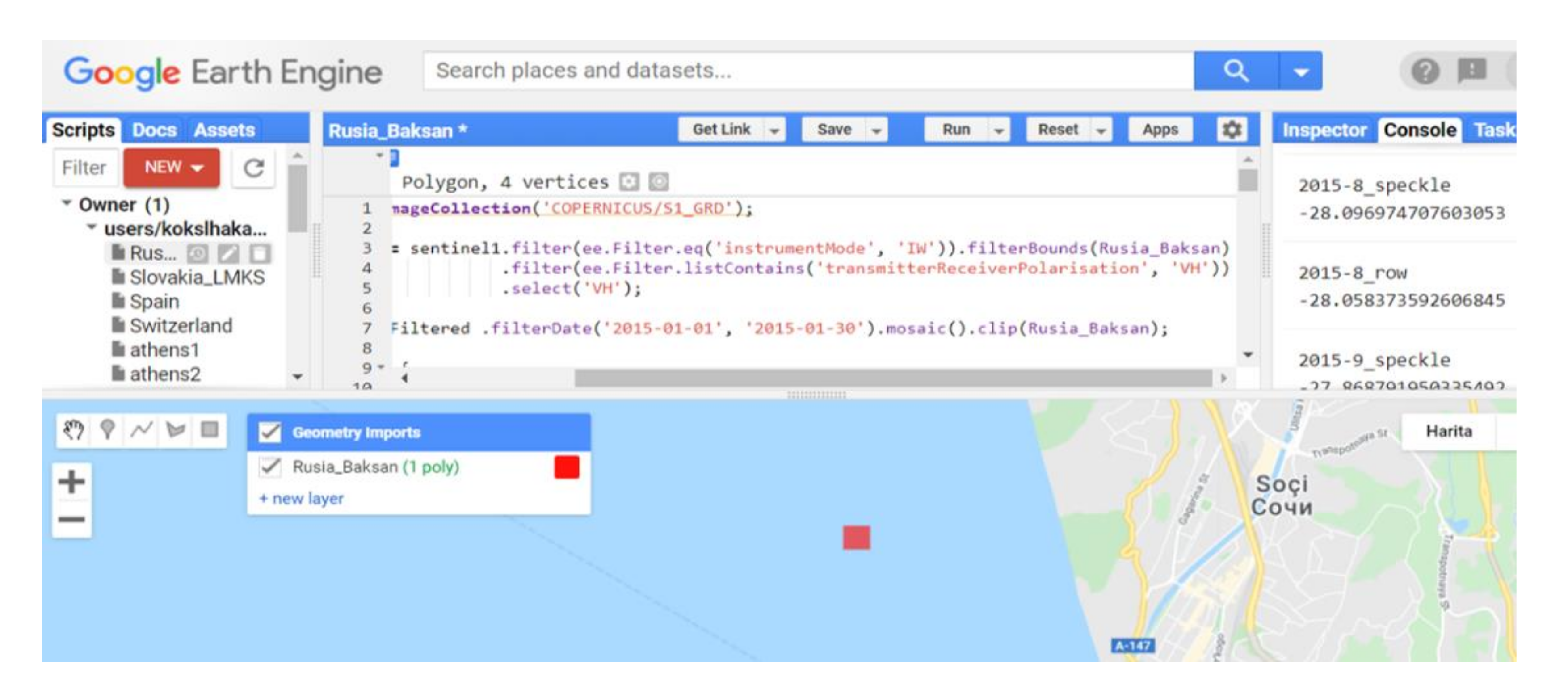
The median values of the differences between the raw radar image data scattering and the filtered image data were calculated and using these values monthly mean median values were produced. The Google Earth Engine (GEE) interface was used for the pre-analysis of the radar data, and the IBM-SPSS software (https://www.ibm.com/products/spss-statistics, accessed on 25 February 2021) for the statistical analysis. For full automated analysis, an interface has been designed to analyze the difference between raw and filtered data which produced in Google Earth Engine Platform (https://earthengine.google.com, accessed on 25 February 2021).
Google Earth Engine is a cloud-based platform for scientific analysis and visualization of petabyte-scale geodata. The data catalog includes observations from various satellite and air imaging systems, at both optical and non-optical wavelengths, environmental variables, weather and climate forecasts and historical forecasts, land cover, topographic and socio-economic datasets. Collections provide quick filtering and sorting capabilities that make it easy for users to search millions of individual images to select data that meet certain spatial, temporal, or other criteria [25].
The JavaScript code editor for the interface is an interactive environment for developing Earth Engine applications. For the Baksan (Russia) test area, the Earth Engine interactive development environment analysis example is shown in Figure 2.
2.4.2. Analysis of the Differences
After the speckle filter was applied, the filtered image data were subtracted from the raw data, and the median of the obtained speckle values was calculated for each month, from November 2014 to December 2019.
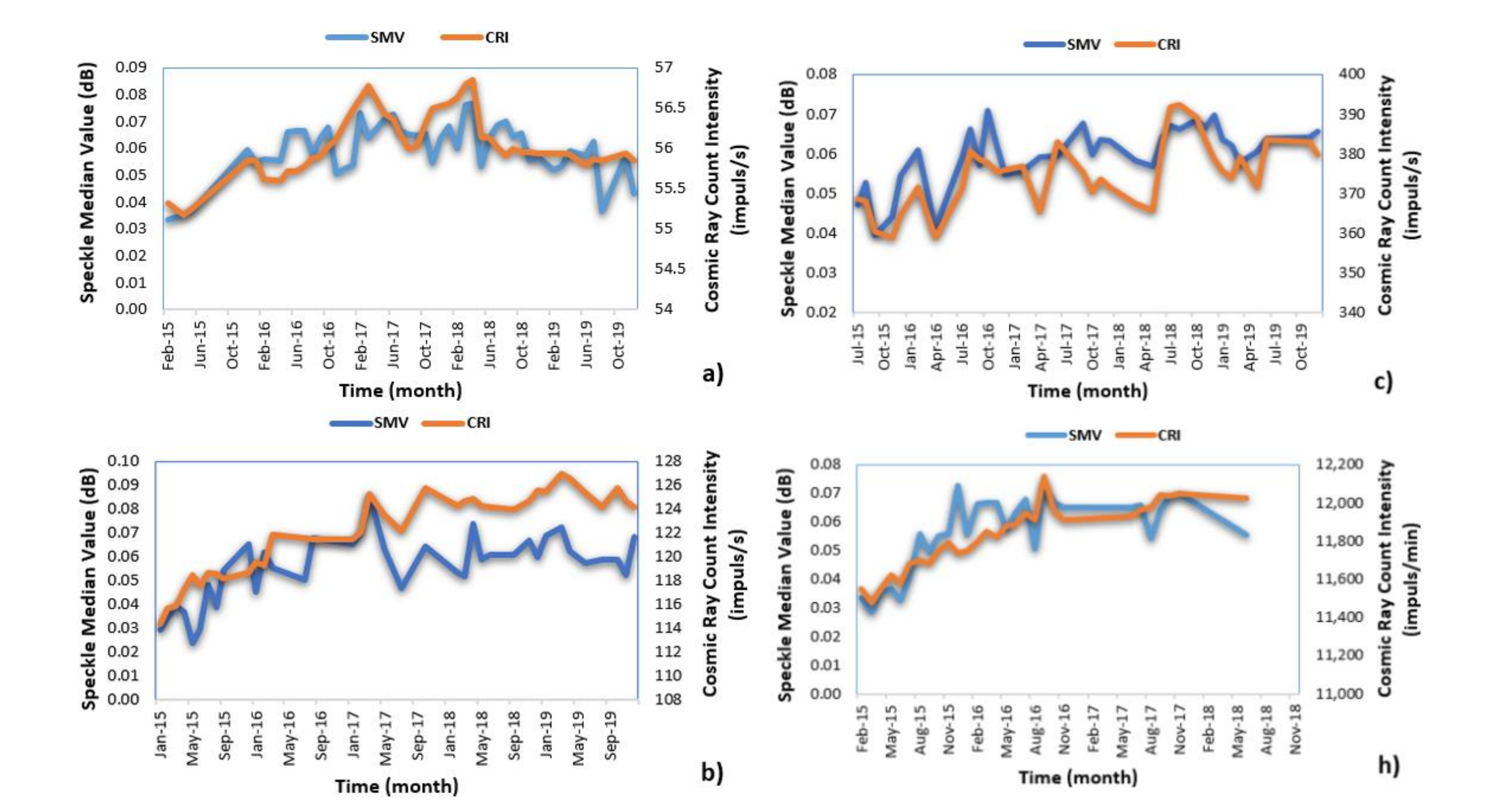
The cosmic ray intensity (CRI) and speckle median values (SMVs) are plotted with the calculated median values of the monthly speckles (Figure 3).
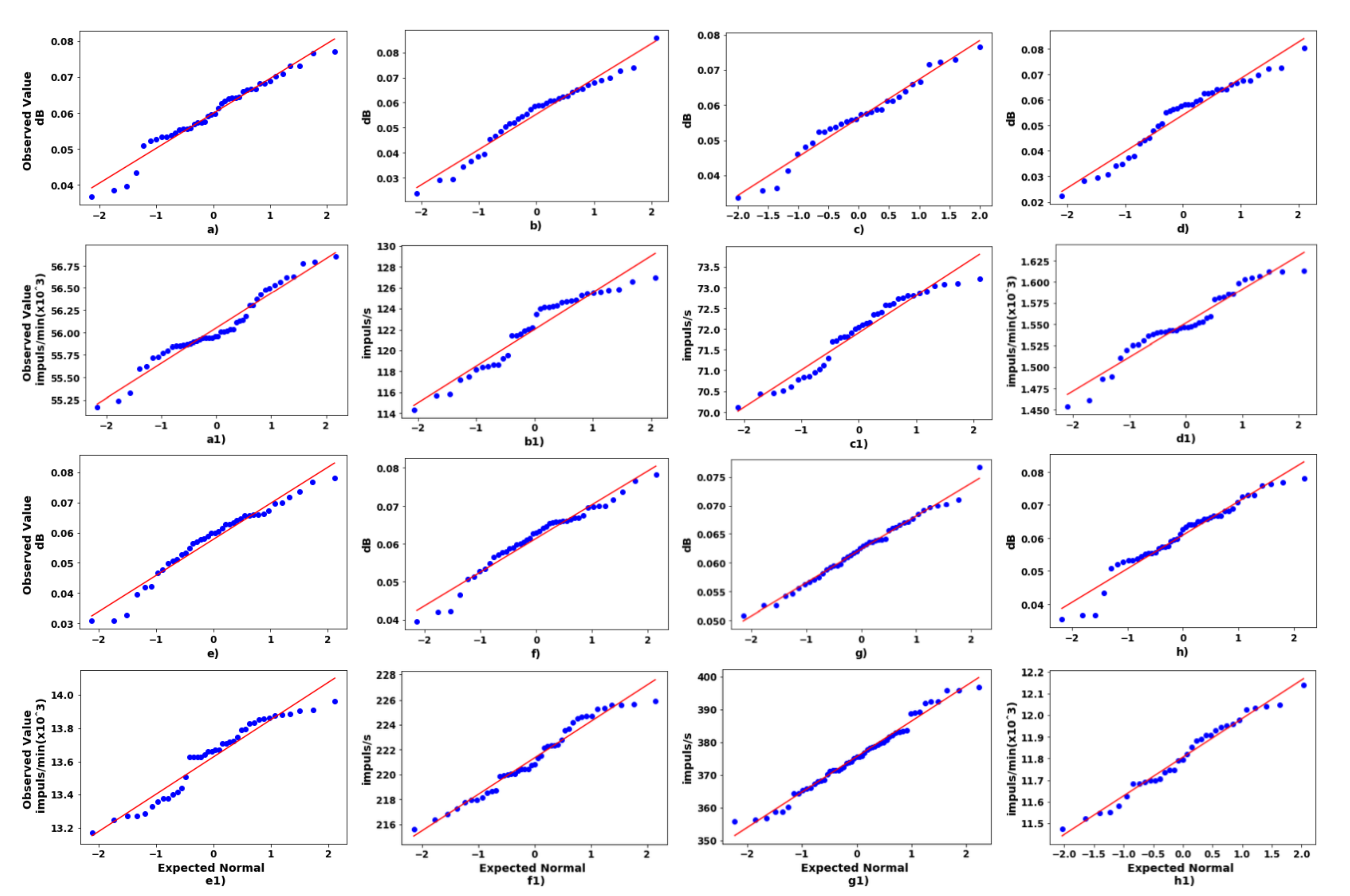
Correlation analysis is one of the most important statistical methods used to determine the degree and direction of relationship between two datasets. In this study, the Pearson correlation analysis method was applied to monthly speckle median and cosmic ray number intensity data, and the correlation coefficient between the two datasets was calculated. IBM-SPSS software was used to test whether the datasets show normal distribution or not. For the determination of the normal distribution, the skewness and kurtosis values should be in the range of ±1.5, and the skewness and kurtosis indices calculated by dividing these values by their standard errors should be to 0 within ±2 limits [26]. In addition, Q–Q charts that reveal the harmony between expected and observed values as a graphical evaluation were examined.
3. Results and Discussion
The temporal change graphs of monthly scatter values and cosmic ray station data obtained for the test areas on radar images are here analyzed. Skewness and kurtosis values obtained as a result of numerical and graphical normal distribution analysis are given in Table 4. As shown in Figure 3, the cosmic ray intensity and the speckle amount have similar distribution curves when doing a visual interpretation.
Q–Q charts that show the normal distribution between expected and observed values are shown (Figure 4). Q–Q plots are used to check if the data have a normal distribution.
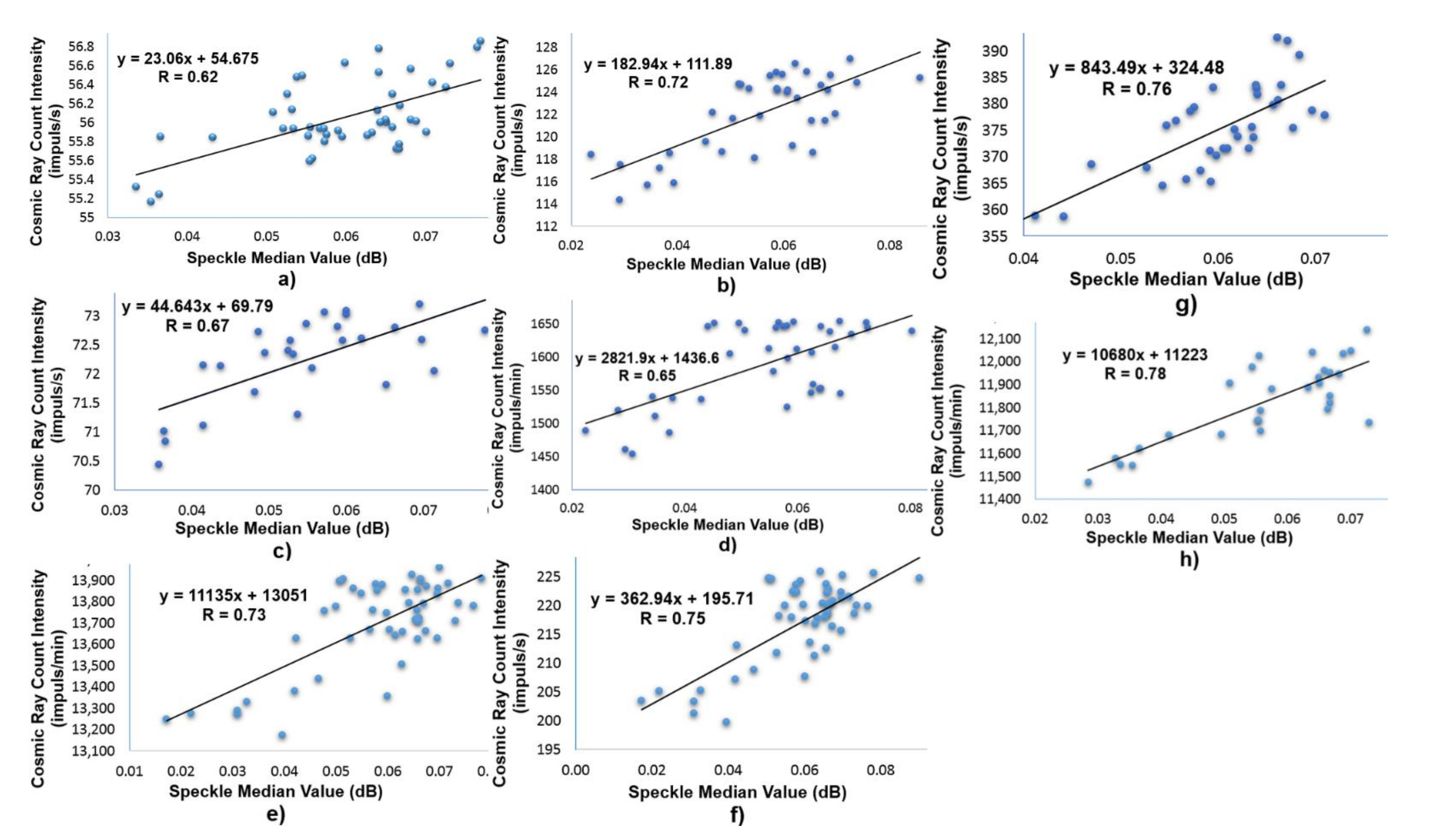
The graphs of variation and correlation coefficients of the two datasets obtained as a result of the Pearson correlation analysis performed for the data of all test areas are shown in Figure 5.
In this study, we aimed to perform the analysis of the effect of high-energy cosmic rays on Sentinel 1 radar satellite images based on the entire Sentinel 1 data catalog, using cosmic ray station data located at different latitudes. During the study, it was seen that the radar data of the dates that were not provided through the Sentinel Copernicus Open Hub (https://scihub.copernicus.eu, accessed on 25 February 2021) open-source data download service were also available in the Google Engine data catalog and using monthly average values to reduce the number of the dates for which there was no data is thought to provide more homogeneous results. Although the method proposed here is automatic, it is based on the principle of performing radiometric and statistical analysis of multi-time satellite images at a certain temporal and spatial scale. The Google Earth Engine interface data catalog, where spatial and radiometric preliminary analysis processes are carried out, includes observations from various satellite and air imaging systems at both optical and non-optical wavelengths, environmental variables, weather and climate forecasts and historical predictions [25]. Therefore, the proposed method will facilitate the examination of similar atmospheric effects for optical satellite images or other factors that may affect reflection values in satellite images in long time periods and spatial limits. In order to reduce the speckle effect on radar images, the Lee filter was used, as it can take into account the speckle distribution model and provide better results, as compared to non-adaptive filters, in terms of calculating local statistics in a moving window [23].
When temporal-change graphs are examined, both datasets show the maximum value on the same dates for Athens, Mexico City, Nain and Tsumeb stations (Figure 3 and Table 5). In addition, it was observed that there is a similar trend (trend) in the increasing direction in both dataset-change graphs.
Pearson correlation analysis was applied to determine the degree and direction of agreement between the two datasets’ temporal variation, and significant correlation values were obtained. In addition, when the results of the Athens Neutron Monitor Station (ANeMoS) with direct count resolution per second obtained through the ESA Neutron Monitor Service were examined, it was observed that the correlation of speckle between cosmic ray intensity is stronger as the average cosmic ray number density increases (Table 6).
Similar to the conclusion we reached in our study, Y’acob et al. [7] investigated the effects of space radiation on satellites in LEO (low Earth orbit) and found that the effects on satellites with space radiation increased linearly due to the orbit height [8]. Therefore, the fact that correlation analysis can be used in the analysis of space weather effects has been supported by our study. The effects of the Ionospheric layers, where cosmic rays and solar radiation effects are seen intensely, on L-band ALOS-PALSAR satellite data were examined in Reference [27]. It has been reported that the ionosphere causes noise in the data, but it is not remarkable. In our study, similarly calculated speckle values were calculated in small amounts, but seeing this effect also has the potential to benefit in space air modeling studies. In the study by Mannix et al. [28], in contrast to the station data we used in our study, ionospheric effects in the L band SAR data were compared with the GPS data in the test areas, as the observed effects on the both datasets are highly correlated. In our study, according to this approach, the consistency shown with the changes in GPS values can be monitored in the next stages, to support the correlation between noise on SAR images and the cosmic number density. The correlation values obtained for the test areas can be seen in the Table 7.
4. Conclusions
In this study, the temporal variation of speckle values in radar images was compared with cosmic ray number density data, to examine the effect of cosmic rays on Sentinel 1 satellite images. In accordance with this purpose, all available radar images in GRD (Ground Range Detected) format with the same scanning angle and VH polarization between January 2015 and December 2019 were filtered and processed on the Google Earth Engine interface, to be used in the analysis. The amount of speckle on radar images was compared with the cosmic ray intensity for all test areas. The analysis results showed a similar trend for the whole dataset (speckle and cosmic ray intensity) and significant positive correlation values which vary between 0.62 and 0.78. Both similar trends and high positive correlations show that cosmic rays interact within the CCD sensors on the satellite and some pixels are oversaturated. Because these particles have very high energy, they can penetrate inside the electronics of the instrument and produce some additional noise in the measurements. Thus, we may conclude that the amount of the difference between measurements is directly related to the number of cosmic rays interacting with the satellite or the observed area, but it needs further research.
The implemented source codes on GEE are available (shorturl.at/kyMN7, accessed on 25th February 2021) for the future observations, to allow the researchers do their own experiments. Out next studies may include an analysis of the effects on the different wavelengths, such as X or L, and continuing the investigations also on the surfaces rather than water.
Author Contributions
Conceptualization, N.D. and A.K.; methodology, N.D.; software, H.K.; validation, H.K., A.K. and N.D.; formal analysis, A.K.; investigation, H.K.; data curation, HK.; writing—original draft preparation, N.D., H.K.; writing—review and editing, N.D.; visualization, H.K.; supervision, N.D.; project administration, N.D.; funding acquisition, N.D. All authors have read and agreed to the published version of the manuscript.
Funding
This work was funded by the Scientific and Technological Research Council of Turkey (TÜBİTAK), Grant No. 119Y072.
Institutional Review Board Statement
Not applicable.
Informed Consent Statement
Not applicable.
Data Availability Statement
Data is contained within the article or supplementary material.
Conflicts of Interest
The authors declare no conflict of interest.
References
- Howell, E. What Are Cosmic Rays? Available online: https://www.space.com/32644-cosmic-rays.html (accessed on 19 December 2020).
- Smart, D.F.; Shea, M.A. Galactic cosmic radiation and solar energetic particles. In Handbook of Geophysics and the Space Environment; Air Force Geophysics Laboratory: Bedford, MA, USA, 1985; pp. 6–29. [Google Scholar]
- Horne, R.B.; Glauert, S.A.; Meredith, N.P.; Boscher, D.; Maget, V.; Heynderickx, D.; Pitchford, D. Space weather impacts on satellites and forecasting the Earth’s electron radiation belts with SPACECAST. Space Weather 2013, 11, 169–186. [Google Scholar] [CrossRef] [Green Version]
- Kocaman, B. Uydularımız Tehdit Altında-Uzay Radyasyonu (In Turkish). TUBITAK Bilim Tek. 2018, 630, 49–63. [Google Scholar]
- Nwankwo, V.U.J.; Jibiri, N.N.; Kio, M.T. The Impact of Space Radiation Environment on Satellites Operation in Near-Earth Space. In Satellites Missions and Technologies for Geosciences; IntechOpen: London, UK, 2020. [Google Scholar]
- Fajardo, I.; Lidtke, A.A.; Bendoukha, S.A.; Gonzalez-Llorente, J.; Rodríguez, R.; Morales, R.; Faizullin, D.; Matsuoka, M.; Urakami, N.; Kawauchi, R.; et al. Design, Implementation, and Operation of a Small Satellite Mission to Explore the Space Weather Effects in LEO. Aerospace 2019, 6, 108. [Google Scholar] [CrossRef] [Green Version]
- Ya’acob, N.; Zainudin, A.; Magdugal, R.; Naim, N.F. Mitigation of space radiation effects on satellites at Low Earth Orbit (LEO). In Proceedings of the 6th IEEE International Conference on Control System, Computing and Engineering ICCSCE2016, Penang, Malaysia, 25–27 June 2016; pp. 56–61. [Google Scholar]
- Allen, J.H. Satellite Anomalies, Recent Events, and Possible Causes. In Space Weather Study Using Multipoint Techniques; Elsevier: Amsterdam, The Netherlands, 2000. [Google Scholar]
- Harboe-Sørensen, R.; Daly, E.; Teston, F.; Schweitzer, H.; Nartallo, R.; Perol, P.; Vandenbussche, F.; Dzitko, H.; Cretolle, J. Observation and analysis of single event effects on-board the SOHO satellite. In Proceedings of the RADECS 2001 6th European Conference on Radiation and Its Effects on Components and Systems (Cat. No.01TH8605), Grenoble, France, 10–14 September 2001; pp. 37–43. [Google Scholar]
- Koons, H.C.; Chen, M.W. An Update on the Statistical Analysis of MILSTAR Processor Upsets. In Proceedings of the Government Microcircuit Applications, Monterey, CA, USA, 3 August–3 November 1999; pp. 816–819. [Google Scholar]
- Koons, H.C.; Fennel, J.F. Space Weather Effects on Communications Satellites. URSI Radio Sci. Bull. 2006, 316, 27–41. [Google Scholar]
- Katz, I.; Mandell, M.; Jongeward, G.; Gussenhoven, M.S. The importance of accurate secondary electron yields in modeling spacecraft charging. J. Geophys. Res. 1986, 91, 13739–13744. [Google Scholar] [CrossRef] [Green Version]
- Vampola, A.L. Thick dielectric charging on high-altitude spacecraft. J. Electrostat. 1987, 20, 21–30. [Google Scholar] [CrossRef]
- Koons, H.C.; Mazur, J.E.; Selesnick, R.S.; Blake, J.B.; Fennell, J.F.; Roeder, J.L.; Anderson, P.C. The impact of the space environment on space systems. In Proceedings of the 6th Spacecraft Charging Technology Conference, Logan, UT, USA, 1 September 2000; Volume 670, p. 1. [Google Scholar]
- Elvidge, S.; Godinez, H.; Angling, M.J.; Koller, J. Improved Modelling of Upper Atmospheric Densities using Multi-Model Ensembles. In Proceedings of the 3rd IMA Mathematics in Defence Conference, Malvern, UK, 23–24 October 2013. [Google Scholar]
- Radicella, S.M. Ionosphere/Positioning and Telecommunications. In Space Weather Research Towards Applications in Europe; Lilensten, J., Ed.; Springer: Berlin/Heidelberg, Germany, 2007; pp. 125–127. [Google Scholar]
- Akioka, M.; Nagatsuma, T.; Miyake, W.; Ohtaka, K.; Marubashi, K. The L5 mission for space weather forecasting. Adv. Space Res. 2005, 35, 65–69. [Google Scholar] [CrossRef]
- Goodman, J.W. Some fundamental properties of speckle. J. Opt. Soc. Am. 1976, 66, 1145–1150. [Google Scholar] [CrossRef]
- Lee, J.S.; Jurkevich, I.; Dewaele, P.; Wambacq, P.; Oosterlinck, A. Speckle filtering of synthetic aperture radar images: A review. Remote Sens. Rev. 1994, 8, 313–340. [Google Scholar] [CrossRef]
- Bruniquel, J.; Lopes, A. Multi-variate optimal speckle reduction in SAR imagery. Int. J. Remote Sens. 1997, 18, 603–627. [Google Scholar] [CrossRef]
- Gagnon, L.; Jouan, A. Speckle Filtering of SAR Images: A Comparative Study Between Complex-Wavelet-Based and Standard Filters. In Proceedings of the Wavelet Applications in Signal and Image Processing V, San Diego, CA, USA, 30 July–1 August 1997; pp. 199–200. [Google Scholar]
- Köksal, H.; Demir, N.; Kilcik, A. Investigation of the cosmic ray effects on sentinel-1 SAR images. In Proceedings of the 41st Asian Conference on Remote Sensing, Online, 9–11 November 2020. [Google Scholar]
- Dong, Y.; Milne, K.A.; Forster, B.C. A sar speckle filtering algorithm towards edge sharpening. Int. Arch. Photogramm. Remote Sens. 2000, 33, 89–95. [Google Scholar]
- Lee, J. Sen Refined filtering of image noise using local statistics. Comput. Graph. Image Process. 1981, 15, 380–389. [Google Scholar] [CrossRef]
- Gorelick, N.; Hancher, M.; Dixon, M.; Ilyushchenko, S.; Thau, D.; Moore, R. Google Earth Engine: Planetary-scale geospatial analysis for everyone. Remote Sens. Environ. 2017, 202, 18–27. [Google Scholar] [CrossRef]
- Tabachnick, B.G.; Fidell, L.S. Using Multivariate Statistics, 6th ed.; Pearson: London, UK, 2012; ISBN 0205849571. [Google Scholar]
- Pi, X. Ionospheric Effects on Spaceborne Synthetic Aperture Radar and a New Capability of Imaging the Ionosphere From Space. Space Weather 2015, 13, 737–741. [Google Scholar] [CrossRef]
- Mannix, C.R.; Belcher, D.P.; Cannon, P.S. Measurement of Ionospheric Scintillation Parameters from SAR Images Using Corner Reflectors. IEEE Trans. Geosci. Remote Sens. 2017, 55, 6695–6702. [Google Scholar] [CrossRef]
Figure 1.
Selecting the pixels from water surface (example from test area, Athens).

Figure 2.
Processing of Synthetic Aperture Radar (SAR) image on Google Earth Engine Platform.

Figure 3.
Temporal variation graphs of speckle median values and cosmic ray number intensity values: (a) Athens (Greece), (b) Baksan (Russia), (c) NM64 NM Jungfraujoch (Switzerland) and (d) Tsumeb (Namibia).
Figure 3.
Temporal variation graphs of speckle median values and cosmic ray number intensity values: (a) Athens (Greece), (b) Baksan (Russia), (c) NM64 NM Jungfraujoch (Switzerland) and (d) Tsumeb (Namibia).

Figure 4.
Q–Q scatter plots of monthly mean speckle values and cosmic ray number intensity data: (a,a1) Athens (Greece), (b,b1) Baksan (Russia), (c,c1) Castilla–La Mancha (Spain), (d,d1) Lomnicky_stit (Slovakia), (e,e1) Mexico City (Mexico), (f,f1) Nain (Canada), (g,g1) NM64 NM Jungfraujoch (Switzerland) and (h,h1) Tsumeb (Namibia).

Figure 5.
Variation of monthly speckle median and cosmic ray number intensity; (a) Athens (Greece) (b) Baksan (Russia). (c) Castilla–La Mancha (Spain) (d) Lom-; nicky-stit (Slovakia) (e) Mexico City; (Mexico) (f) Nain (Canada) (g) NM64; Jungfraujoch (Switzerland) (h) Tsumeb (Namibia).
Figure 5.
Variation of monthly speckle median and cosmic ray number intensity; (a) Athens (Greece) (b) Baksan (Russia). (c) Castilla–La Mancha (Spain) (d) Lom-; nicky-stit (Slovakia) (e) Mexico City; (Mexico) (f) Nain (Canada) (g) NM64; Jungfraujoch (Switzerland) (h) Tsumeb (Namibia).


Table 1.
Number of processed images and time periods.
| Test Area | Number of Processed Images | Time Period |
|---|---|---|
| Athens | 376 | February 2015–December 2019 |
| Baksan | 304 | February 2015–December 2019 |
| Castilla–La Mancha | 224 | May 2015–April 2018 |
| Lomnicky | 312 | January 2015–November 2019 |
| Mexico City | 408 | January 2015–December 2019 |
| Nain | 400 | January 2015–Dcember2019 |
| Jungfraujoch | 288 | July 2015–December 2019 |
| Tsumeb | 240 | February 2015–June 2018 |
Table 2.
Detectors used and cutoff rigidity values.
| Station | Detector | Cutoff Rigidity | Operation Start Date |
|---|---|---|---|
| Athens | 6-NM64 | 8.53 GV | 2000 |
| Baksan | 6NM64 | 5.6 GV | 2003 |
| Castilla–La Mancha | 15-NM64 | 6.95 GV | 2012 |
| Lomnicky_stit | 8-SNM15 | 3.84 GV | 1981 |
| Mexico City | 6-NM-64 | 8.2 GV | 1990 |
| Nain | 63-NM-64 | 0.3 GV | 2000 |
| Jungfraujoch | 3-NM64 | 4.5 GV | 1986 |
| Tsumeb | 18-NM64 | 9.15 GV | 1976 |
Table 3.
The test areas with their locations.
| Test Area | Latitude | Longitude |
|---|---|---|
| Athens | 37°55′34.44′′ E | 23°40′05.74′′ N |
| Baksan | 39°38′32.91′′ E | 43°35′7.50′′ N |
| Castilla–La Mancha | 0°32′15.44′′ E | 40°26′22.40′′ N |
| Lomnicky | 20°16′43.93′′ E | 49°26′23.20′′ N |
| Mexico City | 94°54′54.78′′ W | 29°7′58.35′′ N |
| Nain | 138°41′1.10′′ W | 58°54′22.13′′ N |
| Tsumeb | 22°34′36.33′′ E | 34°1′1.94′′ S |
| Jungfraujoch | 8°24′7.88′′ E | 47°0′58.86′′ N |
Table 4.
Skewness and kurtosis values (SD, speckle amount; CRI, cosmic ray intensity).
| Test Site and Data | Skewness | Kurtosis | Skewness Standard Deviation | Kurtosis Standard Deviation |
|---|---|---|---|---|
| Athens–SD | 0.186 | −0.858 | 0.350 | 0.688 |
| Athens–CRI | −0.240 | 0.054 | 0.333 | 0.656 |
| Baksan–SD | −0.504 | 0.026 | 0.388 | 0.759 |
| Baksan–CRI | −0.393 | −0.802 | 0.347 | 0.681 |
| Castilla–La Mancha–SD | −0.533 | −0.445 | 0.421 | 0.821 |
| Castilla–La Mancha–CRI | −0.447 | −1.016 | 0.374 | 0.733 |
| Lomnicky–SD | −0.552 | −0.494 | 0.383 | 0.750 |
| Lomnicky–CRI | −0.442 | 0.247 | 0.393 | 0.768 |
| Mexico City–SD | −0.673 | 0.072 | 0.374 | 0.733 |
| Mexico City–CRI | −0.603 | −0.825 | 0.357 | 0.702 |
| Nain–SD | −0.550 | 0.134 | 0.383 | 0.750 |
| Nain–CRI | −0.053 | −1.021 | 0.361 | 0.709 |
| Jungfraujoch–SD | 0.077 | −0.187 | 0.357 | 0.702 |
| Jungfraujoch–CRI | 0.111 | −0.497 | 0.327 | 0,644 |
| Tsumeb–SD | −0.653 | 0.518 | 0.347 | 0.681 |
| Tsumeb–CRI | −0.079 | −0.080 | 0.409 | 0.798 |
Table 5.
The maximum values of both datasets which were seen on the same date.
| Station | Date | Max Speckle Median Value (dB) | Max Cosmic Ray Intensity Value (impuls/s or min *) |
|---|---|---|---|
| Athens | April 2018 | 0.0769 | 56.86 |
| Mexico City | October 2018 | 0.0781 | 13,960 * |
| Nain | September 2019 | 0.090 | 225.88 |
| Tsumeb | September 2016 | 0.073 | 12,141 * |
Table 6.
Average cosmic ray number density and correlation values.
| Station | Average Cosmic Ray Number Density (Impuls/s) | Correlation |
|---|---|---|
| Athens | 55.96 | 62% |
| Baksan | 122.45 | 72% |
| Castilla–La Mancha | 71.92 | 67% |
| Nain | 217.4 | 75% |
| Jungfraujoch | 371.38 | 76% |
Table 7.
Pearson correlation values based on the graphs from Figure 5.
Table 7.
Pearson correlation values based on the graphs from Figure 5.
| Station | Correlation | Station | Correlation |
|---|---|---|---|
| Athens | 62% | Mexico City | 73% |
| Baksan | 72% | Nain | 75% |
| Castilla–La Mancha | 67% | Jungfraujoch | 76% |
| Lomnicky | 65% | Tsumeb | 78% |
Publisher’s Note: MDPI stays neutral with regard to jurisdictional claims in published maps and institutional affiliations. |
© 2021 by the authors. Licensee MDPI, Basel, Switzerland. This article is an open access article distributed under the terms and conditions of the Creative Commons Attribution (CC BY) license (http://creativecommons.org/licenses/by/4.0/).
Share and Cite
MDPI and ACS Style
Köksal, H.; Demir, N.; Kilcik, A. Analysis of the Cosmic Ray Effects on Sentinel-1 SAR Satellite Data. Aerospace 2021, 8, 62. https://0-doi-org.brum.beds.ac.uk/10.3390/aerospace8030062
AMA Style
Köksal H, Demir N, Kilcik A. Analysis of the Cosmic Ray Effects on Sentinel-1 SAR Satellite Data. Aerospace. 2021; 8(3):62. https://0-doi-org.brum.beds.ac.uk/10.3390/aerospace8030062
Chicago/Turabian StyleKöksal, Hakan, Nusret Demir, and Ali Kilcik. 2021. "Analysis of the Cosmic Ray Effects on Sentinel-1 SAR Satellite Data" Aerospace 8, no. 3: 62. https://0-doi-org.brum.beds.ac.uk/10.3390/aerospace8030062
Note that from the first issue of 2016, this journal uses article numbers instead of page numbers. See further details here.