
Accuracy of Noise-Power-Distance Definition on Results of Single Aircraft Noise Event Calculation

1
Scientific-Research Department, National Aviation University, 03058 Kyiv, Ukraine
2
Department of Automation of Designing of Energy Processes and Systems, National Technical University “KPI”, 03056 Kyiv, Ukraine
*
Author to whom correspondence should be addressed.
Aerospace 2021, 8(5), 121; https://0-doi-org.brum.beds.ac.uk/10.3390/aerospace8050121
Submission received: 31 January 2021
/
Revised: 21 March 2021
/
Accepted: 22 March 2021
/
Published: 21 April 2021
(This article belongs to the Special Issue Aviation Sustainability)
Abstract
:Aircraft performance and noise database together with operational weights (depending on flight distances) and operational procedures (including low noise procedures) significantly influence results of noise exposure contour maps assessment in conditions of real atmosphere. Current recommendations of the Standard SAE-AIR1845A allow the definition of flight profiles via solutions of balanced motion equations. However, differences are still supervised between the measured sound level data and calculated ones, especially in assessing the single flight noise events. Some of them are well explained by differences between balanced flight parameters (thrust and velocity first of all) and monitored ones by the traffic control system. Statistical data were gathered to make more general view on these differences and some proposal to use them in calculations has been proven. Besides, the real meteorological parameters provide inhomogeneous atmosphere conditions always, which are quite different from the main assumptions of the SAE-AIR1845A, stipulating inaccuracies of sound level calculations.
1. Introduction
Current recommendations on aircraft noise calculations are defined by ICAO document 9911 [1]. Its methodology applies to long-term average noise exposure only, “… it cannot be relied upon to predict with any accuracy the absolute level of noise from a single airplane movement and should not be used for that purpose”. These recommendations are looking enough for overall noise exposure and impact assessment from the airport activities, used for a number of purposes in aircraft noise management, including the noise zoning around the airports. Current versions of appropriate models and software (INM, ANCON, STAPES, SONDEO, IsoBella, etc., [2,3,4,5,6]) are fully correspondent with these recommendations, all of them were verified by CAEP for their relevance with Doc 9911 [1]. In their structure and main methodical approach existing models are integrated noise models, they combine the assessment module of the flight path parameters necessary for noise calculations and the aircraft noise assessment module itself.
However, a number of national noise regulation rules require single noise event assessment or via LAmax, or via LAE (SEL), or via any other noise descriptor, which is correspondent with separate noise events, particularly with aircraft flying-by. The LAmax is the peak noise level of the event in decibels, the LAeq is the averaged during specific time period sound level, which includes the event in decibels, and the SEL is the average sound level for the event in decibels accounting for both intensity and duration–generally talking exposure. SEL takes all of the energy under the line in a sound pressure level versus a time graph and compressed it to a 1-second value. SEL for each flight operation is then adjusted to reflect the duration of the operation and arrive at a “partial” contribution to noise index LDN (or LDEN) for the operation [1]. The partial LDN are then added logarithmically to determine total noise exposure levels at any point of noise control for the average day of the year. For example, the Sanitary Norms of Ukraine [7] still require for assessment of LAmax together with LAeq during the day (07:00–22:00) and night (22:00–07:00) periods for any type of source, aircraft noise also. Thus, the noise zoning around the airports is defined by calculations of LAmax, LAeq, LDEN (European noise index is also required to be assessed by newish aviation rules of Ukraine APU-381 [8]). The predefined maximum size (area) for any of these criteria should be used for the adoption of appropriate noise zone and protection measures.
Usually, the aircraft fleet and air traffic with appropriate distribution of flights between the routes are necessary input data for aircraft noise calculations. ICAO DOC 9911 guidance [1] for use in Ukraine is somewhat limited in calculating the maximum sound level LAmax and/or sound exposure level LAE, but is mandatory for use in accordance with the requirements of the aviation rules of Ukraine APU-381 [8] for spatial noise zoning around the airport. Complementarily to this any new development inside the specific noise requires the assessment (preferably by measurements) of LAmax together with LAeq at its location for comparison with the norms for this territory and if necessary–to define appropriate protection measures from aircraft noise impact. Follow-up measures–noise monitoring, performed either or as portable or as continuous aircraft noise measurements in the vicinity of airports–must be done at this site and other locations for comparison to show the adequacy of predefined and realized noise protection measures. And once again monitoring (instrumental or calculation-based at sites where measurement terminals are absent) should be provided for the maximum sound level of any peak noise events LAmax, sound exposure level LAE and for the equivalent sound level LAeq (for example, LAeq, logged with a 1 s step usually for current monitoring requirements [9]) for a specific period of the day to inform the population and authorities how the noise norms are fulfilled and if they are still violated—the new measures to protect the people from noise must be proposed. In such a case, the requirements for the accuracy of noise calculation models are quite similar to the accuracy of an instrumental noise assessment.
2. Basic Calculation Equations and Terms
For any particular environmental acoustic source including an aircraft its sound pressure level (SPLΣ) at any point of noise control at distance R from the source [10,11] is defined by the following equation:
where LW is the sound power level for the particular i-th acoustic source of the aircraft under consideration, normalized to the reference distance R0 (usually R0 = 1 m); n–number of acoustic sources with an essential contribution to the overall spectrum of the aircraft at specific flight stage (or flight mode); ΔLΘ is the correction for directivity of sound radiation; ΔLf is the spectral correction for frequency band f; ΔLv is the correction for aircraft speed v; ΔLint is the correction for sound interference corresponding to the “ground” noise attenuation; ΔLscr is the correction for sound diffraction corresponding to noise attenuation by acoustic screen, and α is the sound absorption coefficient in air. The main contributions in this model from the source are defined by LW, ΔLΘ, and ΔLf–these contributions are defined by models of the individual acoustic sources of the aircraft as listed in [10].
The number of acoustic sources that are sufficient for the particular type of aircraft under consideration depends on the type of the engine in its power plant and on aircraft flight mode. The model of dominant acoustic sources for overall aircraft noise assessment TRANOI [10,11] is based on semi-empirical models for them as it is recommended by ICAO Manual [12] and it has quite a high accuracy for spectral and overall SPL assessment ( = ±1.2 dB) of the aircraft in any possible flight event. The use of such a sophisticated acoustic model of the aircraft in a number of noise management tasks is still impossible. It is due to the huge number of input data necessary to calculate all components of the model. All acoustic sources properties of the aircraft under consideration at departure and/or arrival airport, are mostly unavailable for wide usage due to their confidential character (they are protected by the manufacturer of the aircraft and engine).
To simplify the calculation procedures for aircraft noise assessment in and around the airports an approach of Noise-Power-Distance-relationships (NPD-relationships or NPD-dependences) was introduced [1,13], which is still the most common type of acoustic model for aircraft and usually included in integrated noise models and used for calculating the noise levels around airports. For example, the contribution to the sound exposure level LAE from each flight path segment is calculated as follows (Doc 9911 [1], ECAC [13]):
where LE∞(P,d) is the initial value of sound exposure level for the flight segment of infinite length, which is determined based on the interpolation of NPD-dependences data for the actual values of thrust (or power) of the engine P and distance d, corrections are quite similar to corrections of the model (1)–the correction for aircraft speed ΔLv, the correction for directivity of sound radiation ΔLΘ, the correction for sound interference corresponding to the “ground” noise attenuation ΔLint, but they are generalized for total aircraft fleet–not specific to aircraft type. The correction ΔLF is a ratio of sound energy received from a particular segment to the energy received from an infinite flight path, it is used for exposure levels only.
NPD-relationships in model (2) include the sound power level of the aircraft type under consideration and the two last corrections of the model (1) for divergence and absorption of the sound waves in a real atmosphere. Because the sound absorption is frequency-dependent the corrections for sound directivity pattern ΔLΘ and frequency band ΔLf of the noise source also influence NPD-data sufficiently.
A similar concept to NPD-relationships–noise radius RN–is used in a Ukrainian calculation method [11]. It is an extension of the concept of the shortest distance d that is used in NPD-relationships. The moving aircraft is represented as an axially-symmetric noise source, around which the cylindrical surfaces with constant sound levels are formed, such as shown in [10]. For any time-integrated (exposure type) sound levels (or noise indices) at constant flight operational mode and specific magnitude of exposure levels the product RN × v = const, as a function of noise radius RN and flight velocity v only. This result has been verified by different numerical investigations for a variety of aircraft types, even after accounting for the influence of atmospheric absorption in various states of atmosphere. At high flight velocities, airframe noise sources contribute to the magnitude of overall aircraft noise level sufficiently compared to engine noise sources, due to this the relationship RN × v =const is violated. However in most cases of practical interest, the flight velocities do not exceed their critical values at take-off and landing conditions, at least for aircraft with acoustical performances in accordance with the limits of ICAO Chapter 14 [14], so this relationship can be used in calculations and modeling of aircraft noise around airports. The correction to exposure type sound levels for variations of flight velocity v is equal to the ICAO recommendation:
where v0 is the reference velocity usually used for NPD-relationships determination.
3. Historical Development of the Integrated Aircraft Noise Models
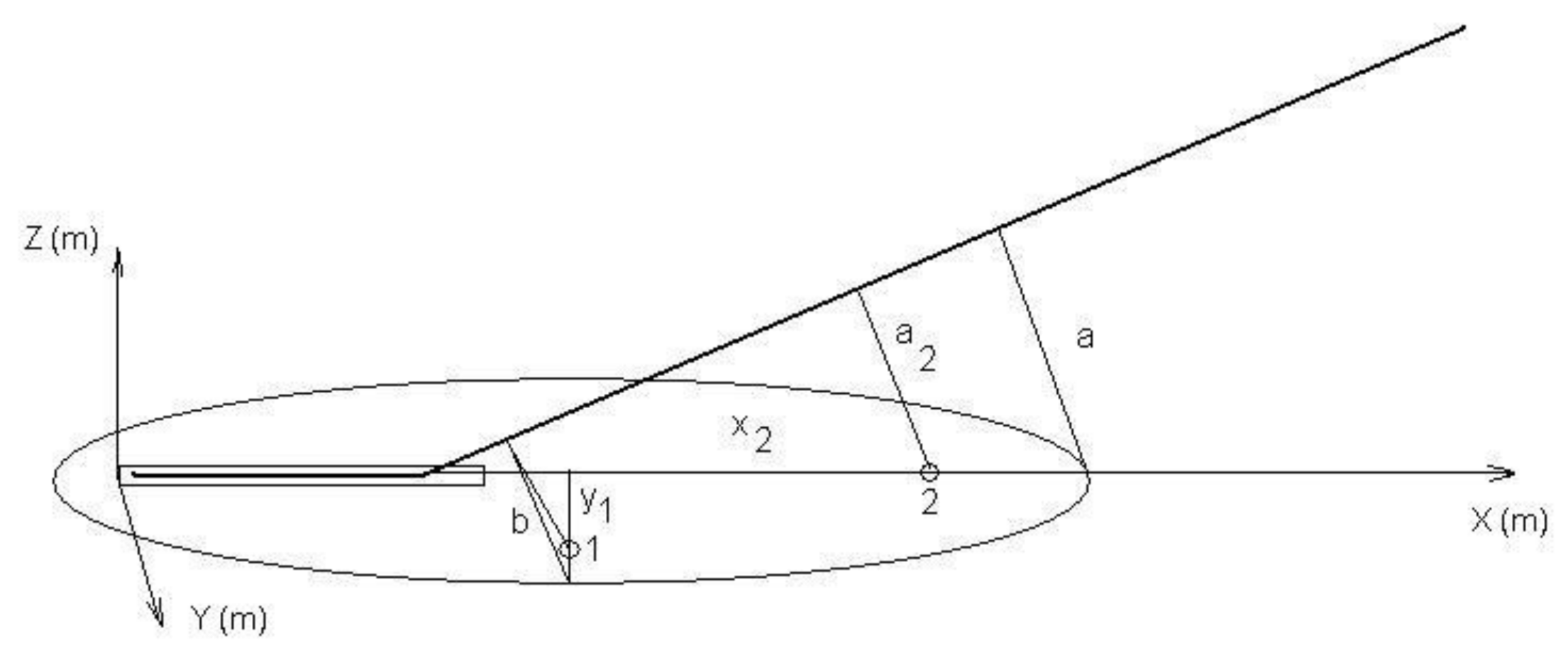
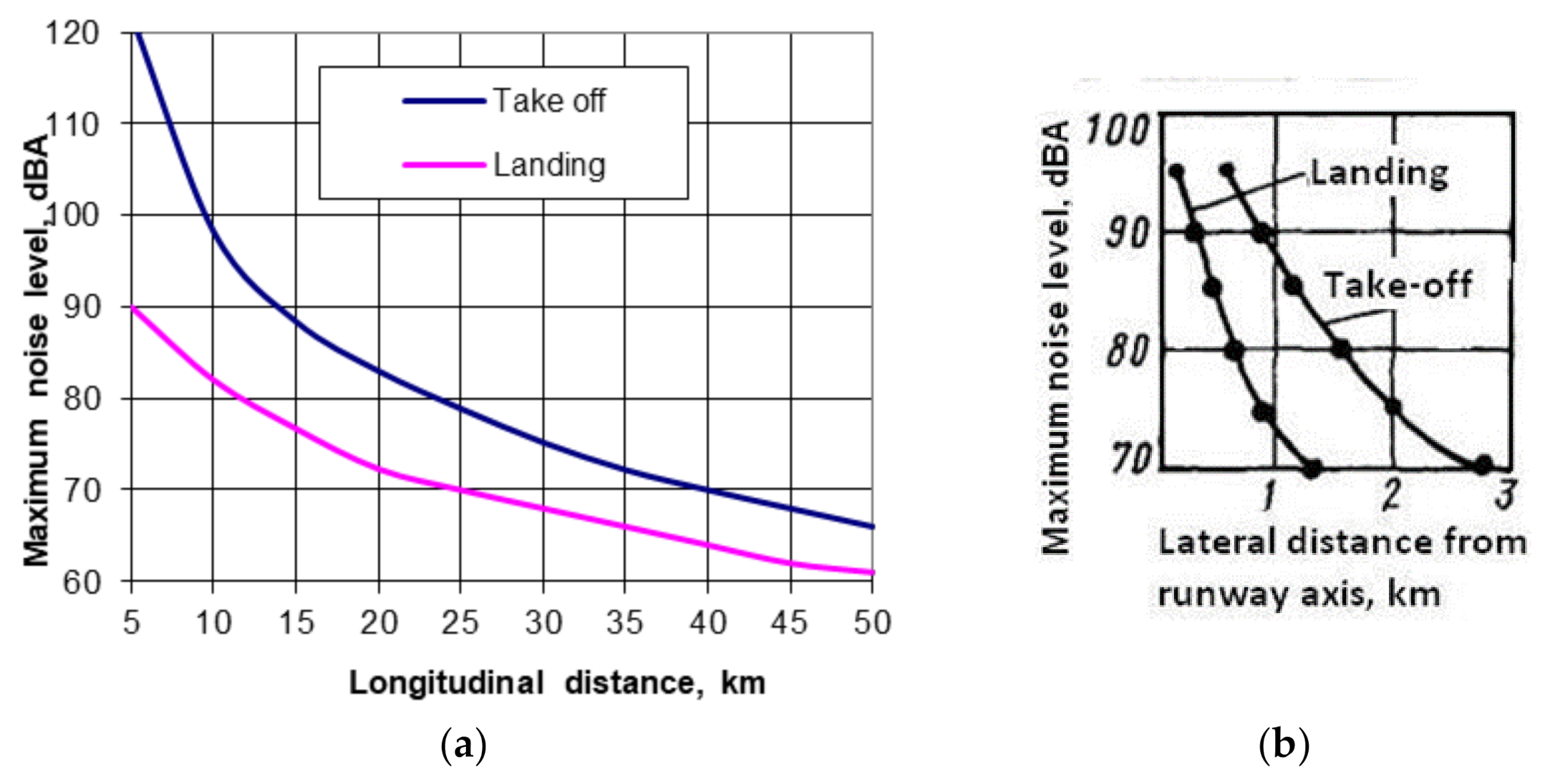
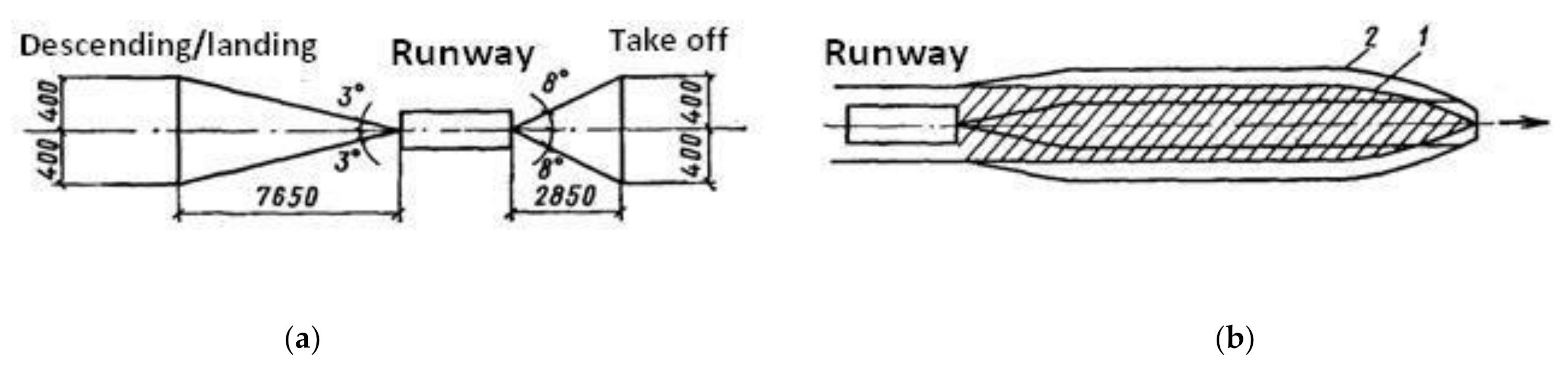
The simplest type of aircraft noise model is confined to the so-called aircraft grouping method and includes the definitions of noise footprints (contours for specified values of noise indices and areas, bounded by these contours—Figure 1) for any group of the aircraft and particular flight stage. Usually, two flight stages were considered as enough for aircraft noise zoning and land use planning around the airports–departures (take-off/climbing) and arrivals (descending/landing) of the aircraft. Flight paths for departure and arrival were defined with respect to the predefined group, for example in the first Soviet Union method [15] there were 5 aircraft groups in a list, a basic group included the Tupolev-134 and Tupolev-154, Iljushin-62, Antonov-10, and Antonov-12 aircraft. The aircraft Antonov-22 and Iljushin-76 were included in the noisiest group, which was on 5 dBA noisier in comparison to the basic group. For all of them besides the averaged flight profiles, there were also averaged relationships of the sound levels from the distance (Figure 2), which were defined from the flight trials, averaged for the group, and used further for noise calculations.
The idea of noise certification of the aircraft was developed at this time, but still not included in consideration to aircraft noise calculation, never mind the direct correlation was shown between the values of sound levels (noise indices) at certification points (Figure 1) and noise footprint area/size for appropriate flight stage [10]. This method defines the appropriate group for the aircraft under consideration depending on the most important operational parameters including take-off mass, number and type of engines in the power plant.
The calculated noise footprints (or contours) were very close to the form of ellipse or part of it, the method of aircraft type grouping predicts noise levels at the point of noise control with an accuracy of ±5 dBA for take-off/climbing and ±3 dBA for landing.
In principal, an ellipse may be defined as a result of the intersection between the plane surface of noise calculation and a cylinder with radius a (shown in Figure 1), where a cylindrical surface is defined by acoustic energy (or acoustic exposure) distributed around the line source of noise generation by aircraft in move along the flight path (or it particular part–flight segment). The difference between the certified noise level at take-off (L2) and the level corresponding to the final point on the contour L along the flight (landing or take-off) axis may be written (taking in mind а/a2 = x/x2):
where the constant C defines the attenuation rate, for spherical spreading its value is near to 20, a is the minimum distance from the flight path to the final point on the contour (Figure 1), a2 is the minimum distance from the take off path to the certification point No. 2 (for take-off). In a same way for the certification sideline point No. 1, the minimum distance b1 enables connection of the certificated level L1 with final point of the (maximum half-width) contour b:
L2 – L = Clg(a/a2) = Clg(x/x2),
L1 – L = Clg(b/b1) = Clg(y/y1).
Since area S is proportional to the product x·y, then, from (4) and (5), it is proportional to L2 and L1:
which is the same as Equation (4.1.1) in [10]. Grounding on Equation (6) one may deduce that for aeroplanes with quite equal certification levels the appropriate footprints will be close to equal also.
lg(S) = (L2 + L1)/C + D,
Very close to linear the relationships between noise contour areas and EPNL values for take-off flight procedures (for EPNL values at control point No. 2) and for landing flight procedures (for EPNL values at control point No. 3), shown in Figure 4.1 in [10], confirm this suggestion and prove the basic idea of the grouping of aeroplanes with similar noise certification data in first noise contour calculation method [15]. The fruitful idea of the aircraft grouping is still used even in current calculation methods [1]. If the necessary for calculation data are absent in database for any aircraft it may be calculated by substitution aircraft, which is definitive for calculated type in particular and for any other type of the aircraft from the group, to which a substitution type is defined.
In the first ICAO document [16] on the subject of aircraft noise calculation, this radius a (Figure 1) was called Noise-Power-Distance relationship (NPD-relationship), taking in mind that for the first jet aircraft its noise was defined by jet engine completely and engine power setting defines also the value of noise level at a specific distance or a value of distance for specific noise level. In a number of works, this radius was called noise radius [10,11]. Because during the specific flight stage (either departure or arrival) the engine operation mode is changing sufficiently an ICAO circular [16], so as an international standard SAE-1845A [17], recommended to divide the flight path on a number of segments with specific engine setting and wing flaps deflections and to use for these settings (power) a specific NPD-relationship (NPD-curve). NPD-curves were defined as aircraft type specific—specific to the aircraft group. It was assumed that the NPD-curve relationship adequately represents the atmosphere state and flight segments in any airport study area. NPD-curves were recommended to be defined during noise certification trials as detailed as it was necessary to cover possible flight modes during the departure and arrival stages of the aircraft type under consideration. Such procedure provided more accurate noise results in comparison with the first aircraft noise calculation method at least on 1–2 dBA [10,11].
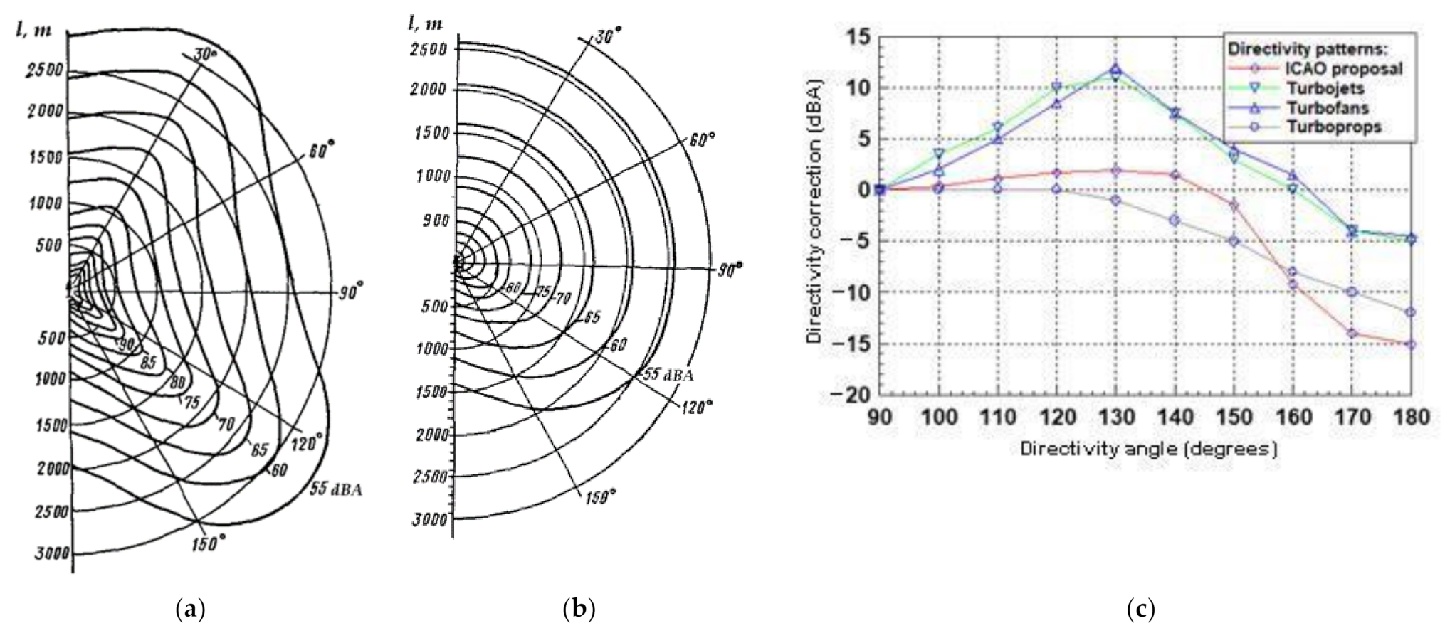
Current ICAO Doc 9911 [1] is much closer to standard SAE-1845A [17], it recommends a number of improvements for the further increase of the accuracy of noise calculations: a number of segments for the flight path is defined by requirements to the change of the flight parameters like flight velocity, wing aerodynamic configuration, and engine thrust, all of them are defined in accordance with meteorological parameters of the case under consideration and flight safety requirements. In a part of noise level calculations, few corrections were introduced: for engine type (jet or propeller, Figure 3), for engine installation (under the wing, over the wing, at the tail of the fuselage), and so-called lateral attenuation effect. In ICAO Doc 9911 the engine type and installation effect are combined in a single correction on engine installation effect (two lateral directivity functions are employed: for aircraft with tail-mounted and wing-mounted engines respectively), two corrections were remained specific–on lateral attenuation and on the directivity of noise propagation from the aircraft (which accounts for the pronounced directionality of jet engine noise behind the ground roll segment, Figure 3). All the corrections in ICAO Doc 9911 [1] and SAE-1845A [17] are used as averaged for the overall aircraft fleet. An ECAC Doc 29 [13] recommends using two corrections on noise directivity –for turbofan-powered jet aircraft and for turboprop-powered aircraft, which contribute essentially for noise footprint contour and area first of all for departure flight noise–at takeoff roll of the aircraft along the runway.
3.1. Lateral Attenuation
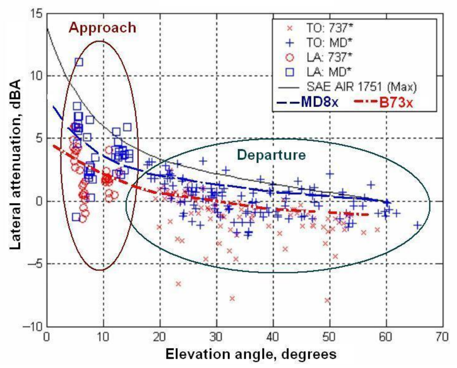
Lateral attenuation due to SAE Standard AIR1751A [18] was processed and presented in a way how overall aircraft noise is attenuated to the side of the aircraft flight pathrelative to the level directly beneath it. The standard equation was derived empirically from a large set of flight noise data based on aircraft types with ICAO Chapter 2 acoustic performances, including and predominantly with tail-mounted engines such the Boeing 727, Lockheed L-1011, Falcon 20, Falcon 50, Douglas DC-9, Douglas DC-10, etc., [18]. The equation for lateral attenuation presented in Standard AIR1751A is calculated as a function of lateral distance d and elevation angle β only [18]—without any difference to the spectrum of noise generated by aircraft and to a surface covering performances over which the effect is observed. This lateral attenuation model is considered as still reliable by SAE 1845A [17] and ICAO Doc 9911 [1], especially for aircraft with tail-mounted engines (Figure 4) but the latest SAE Standard AIR-5662 [19] method recognizes that part of this “lateral attenuation” is, in fact, a lateral directionality associated with engine installation effects. Measurement results even show an amplifying effect for bigger elevation angles as for departures, so as for arrivals. This suggestion was proved the experimental data of the engine installation effects investigation [20] showing the significant differences in the engine installation component of lateral attenuation between jet airplanes with wing-mounted engines and jet airplanes with tail-mounted engines. Possible reasons for these differences are related to the differences in physical geometry of these two groups of airplanes.
By Standard AIR-5662 [19] this attenuation is still termed “lateral attenuation” and is in excess of the attenuation from wave divergence and atmospheric absorption. It is applied to turbofan-powered transport-category airplanes with engines mounted at the rear of the fuselage or under the wings or general-aviation airplanes. Sound wave propagation is considered over “acoustically soft” ground surfaces such as lawn or field grass. So, the method is inconsistent with “acoustically hard” ground surfaces such as frozen or compacted soil, asphalt, concrete, water, or ice.
3.2. NPD-Relationship for Homogeneous Atmosphere
All current software products, such as Integrated Noise Model (the FAA’s Integrated Noise Model–INM–is well known amongst noise modeling specialists), are integrated models because their two basic components–flight path and acoustic modules–are used to assess a complete noise event–a separate flight of the aircraft over the investigated area or a specific noise control point [10,11]. Noise data in their databases are usually supplied by aircraft manufacturers in the form of NPD-curves [1], which are provided for standard values of temperature and humidity and for a homogeneous atmosphere. Different aircraft noise models consider the same physical phenomena but do so with different levels of detalization and different sets of specific computational algorithms. Flight profiles (flight trajectories in the vertical plane) of the aircraft are determined by solving a system of equations of balanced motion recommended by existing methods and standards [1,17], using data for the required coefficients from the ANP database supported by Eurocontrol today (www.aircraftnoisemodel.org, accessed on 2 April 2021). It includes the data for around 200 aircraft types in the database, as for flight profiles, as for noise calculations.
For all the methods the flight profiles are considered in space in accordance with flight routes in the vicinity of the airport (or of the specific runway), which are shown in flight charts for the airport as nominal flight tracks. Accuracy of noise calculations depends on how close to the flight chart track a flight path is realized in a real situation, usually a flight path distribution exists inside a flight corridor (which may be predefined by flight chart for any route as lateral limits relatively to flight track) with axis along the flight track (Figure 5). ICAO Doc 9911 [1] in the current edition provides the calculation scheme of such possible distributions (close to normal distribution), which are important for the calculation of equivalent sound levels and/or day-night noise indices. It is absolutely incorrect for single flyover event noise assessment, which should be closer to real flight trajectory parameters. Taking all this in mind the simplified scheme of any integrated noise model is looking like shown in Table 1.
Today for a number of airports because of their specific aerodrome layout, infrastructure, and much quieter aircraft in operation due to ICAO Balanced Approach influence on acoustic performances of new aircraft designs not only the flight stages contribute essentially on noise footprints inside/around the airport, but taxiing of the aircraft to/from the runway from/to the gates close to terminals may contribute also and must be included in calculations of noise contours to be used for noise zoning purposes. Widespread implementation of Automatic Dependent Surveillance-Broadcast system (ADS-B) [22] onboard the aircraft, which are required by ICAO for safety purposes, first of all, even today simplifies the procedure of aircraft supervising (both in flight and on the ground) providing real data for noise source location necessary for further their noise exposure calculations in/around airports. Currently, the aircrafts are nicely supervised and checked on how they fulfill the flight corridor requirements and due to this, the lateral distribution of real flight trajectory around the flight chart track is very narrow today providing quite a narrow noise footprint in the result.
Differences in the calculation of the integrated models from measured values are the result of an underestimation of the exposure level SEL of the take-off noise of the average aircraft by ~3 dBA and during the descending before landing by ~1.5 dBA. The error of instrumental measurement of sound levels of single flyover events in accordance with the provisions of the modern international standard DIN 45,643 [23] is about 1 dBA, so the discrepancy between the calculated and measured values for individual events is still too large. Investigation of the reasons for underestimation of noise exposure in the calculation of single events of aviation noise radiation and improvement of the model to approach the measured values is one of the main tasks of the research, the practical result of which is to improve calculation-based monitoring of aviation noise at and around the airports.
3.3. Flight Profiles Accuracy
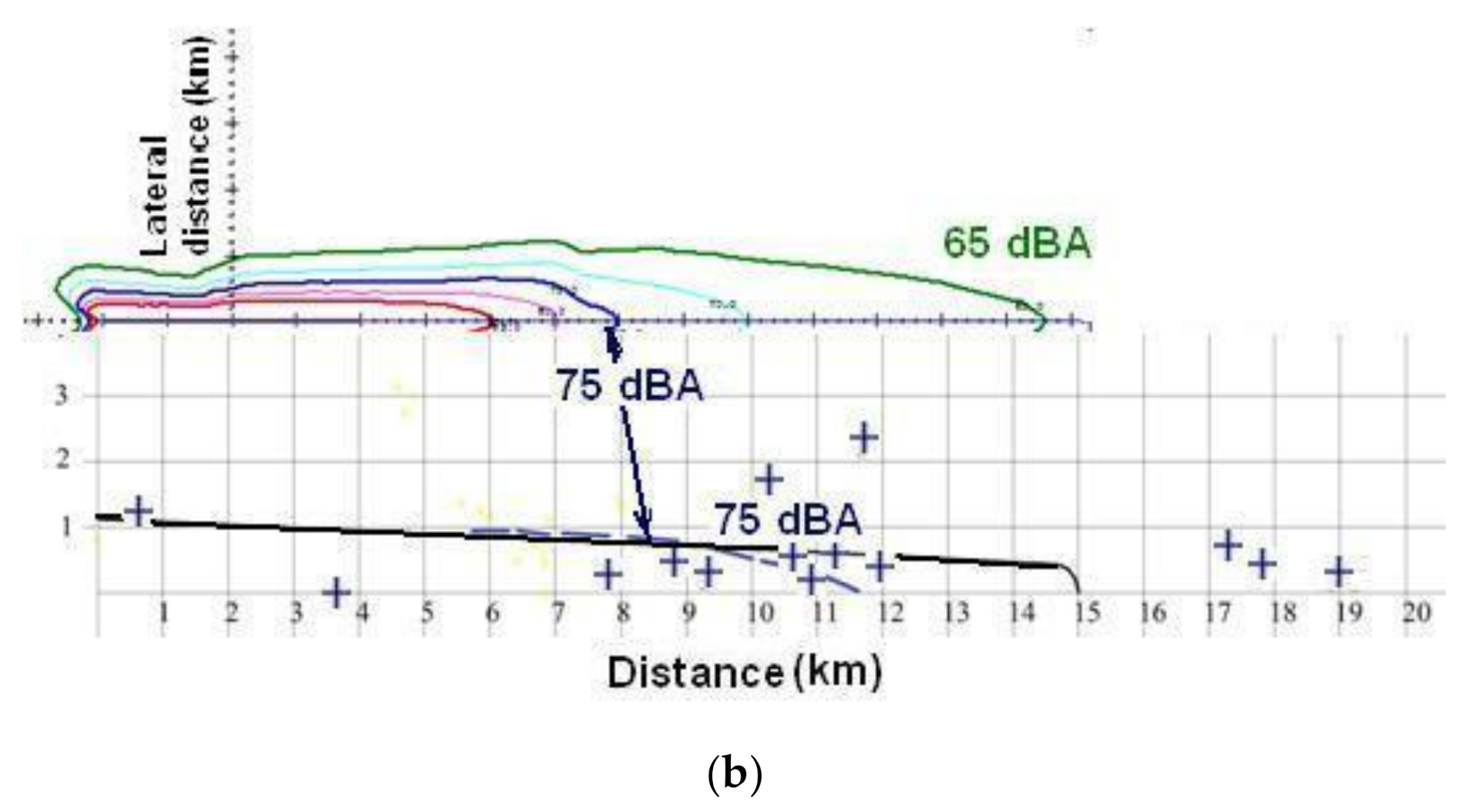
Flight profiles in real operation differ greatly from the results of prediction for balanced motion usually, as for take-off/climbing, so as for descending/landing profiles [21,24]. The differences are observed not only for the height-distance dependences but for the flight speeds and engine thrust settings, which contribute much to the predicted levels of noise also. For the take-off/climbing flight stage noise contour for LAmax = 75 dBA, which is defined by input data for flight parameters observed in operation, may be longer on 3–5 km in comparison to balanced flight input data as shown in Figure 6.
The acoustic basis of any aircraft noise simulation model consists of point sources that move dynamically in time, somewhere, and sometimes represented by line sources along the flight trajectories in horizontal and vertical planes. It includes the effects of geometric propagation (divergence) of sound waves from the source, absorption of their acoustic energy by air, and the effect of their interaction with the earth’s surface (interference of direct and reflected waves from the surface). Different models consider the same physical phenomena but do so with different levels of detalization and different sets of specific computational algorithms.
Flight profiles in real operation differ greatly from the results of prediction for balanced motion usually, as for take-off/climbing, so as for descending/landing profiles (Figure 7). The differences are observed not only for the height-distance dependences but for the flight speeds and engine thrust settings, which contribute much to the predicted levels of noise also (Figure 8).
Review [26] is a good examination of SAE AIR-1845A methodology, realized in the ANP database and both standards [1,17]. The FAA linear regression method for the calculation of aerodynamic and flight performance coefficients was tested, validated, and refined for the six study airplanes. As the regression is developed using procedures for a wide range of airport altitudes, airplane weights, and atmosphere temperatures, the resulting coefficients can reproduce flight profiles over a similar range of conditions. A key attribute of the FAA method is the use of the manufacturer’s flight profile data directly, which are easier and more intuitive for the industry to produce than the ANP database coefficients. This distinction also simplifies error checking, and the bounds of the matrix of flight profile data determine the range of applicability of the coefficients.
3.4. Arrival Flight Profile Parameter Analysis
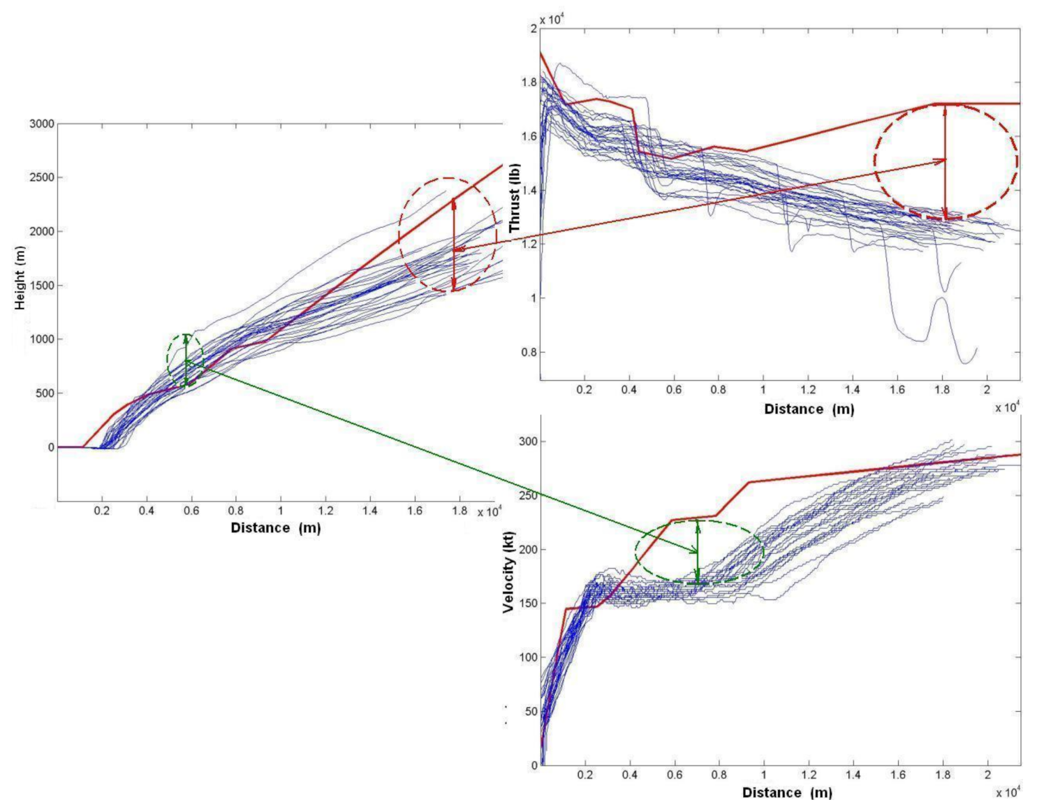
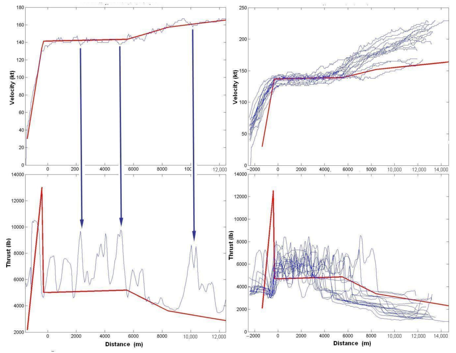
In Figure 9 (combined from four figures, which were taken from [21]) the data for arrivals for two types of aircraft are shown. If to look at the flight speed (on the top of Figure 9) it should be found that operational speeds (blue lines) vary along the glide path and sometimes their values may be reduced below the flight safety requirements (value of balanced flight solution, which is defined in accordance with safety requirements also, is shown as a red line in Figure 9 at the top-left picture). In these cases a pilot must operate with thrust, making engine operation mode higher, trying to return the speeds to the safe values–so in reality we must consider overbalanced thrusts (due to flight control from pilot to return the velocity into safe diapason—by arcs every reduced velocity in the top left picture is connected with an increased thrust of the engine in the bottom left picture in Figure 10). It was found that the thrusts may be two-times higher than the balanced predictions for them. For some types of aircraft, the balanced predictions were found much less than observed thrust in operation (Figure 10, on the right), which may be accessed as a mistake in input values for coefficients (aerodynamic or thrust) in used databases.
By correction of the thrust at final glide slope descend for B-734 the LAmax is higher on 9–10 dBA than for similar ANP database result. Because of the very close location of this difference i9n flight operation to the runway, it influences the smaller in size contour 85 dBA making it 1–2 km longer as calculated by the IsoBella model and software (Figure 10). For smaller LAmax the contours are not affected sufficiently by these flight control measures. If balanced thrust and speed are seriously different from their measured and averaged values (Figure 10, on the right) the influence of this difference will be observed for all the contours (65–85 for LAmax) under investigation, not only for the smallest ones (for higher LAmax).
3.5. Departure Flight Profile Parameter Analysis
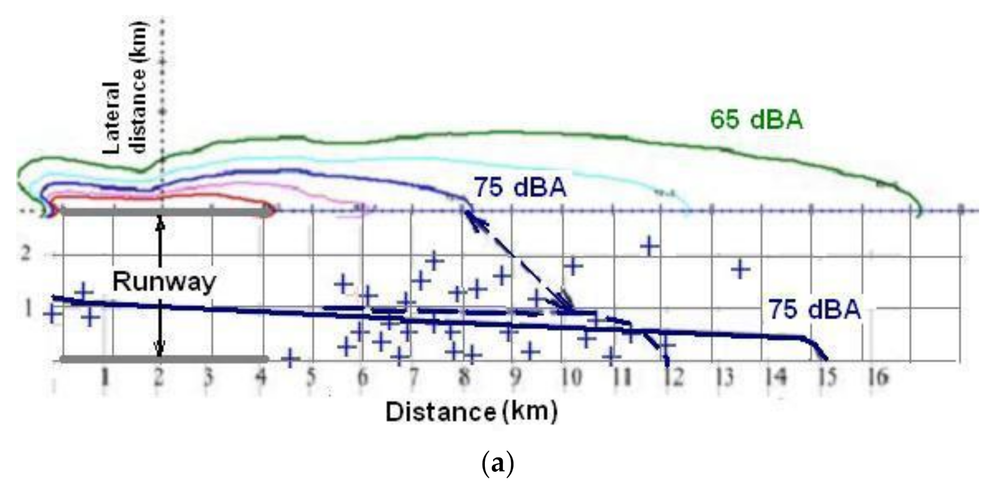
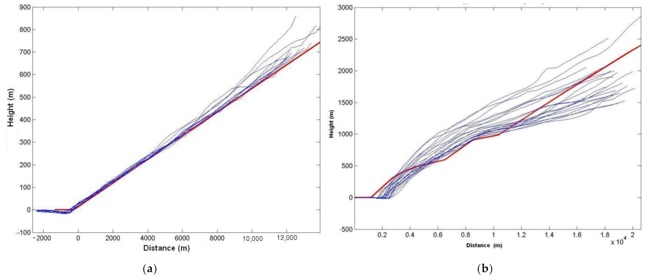
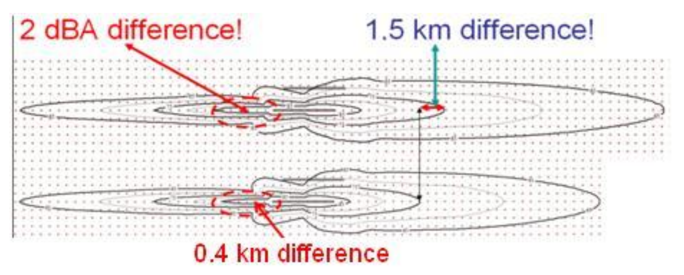
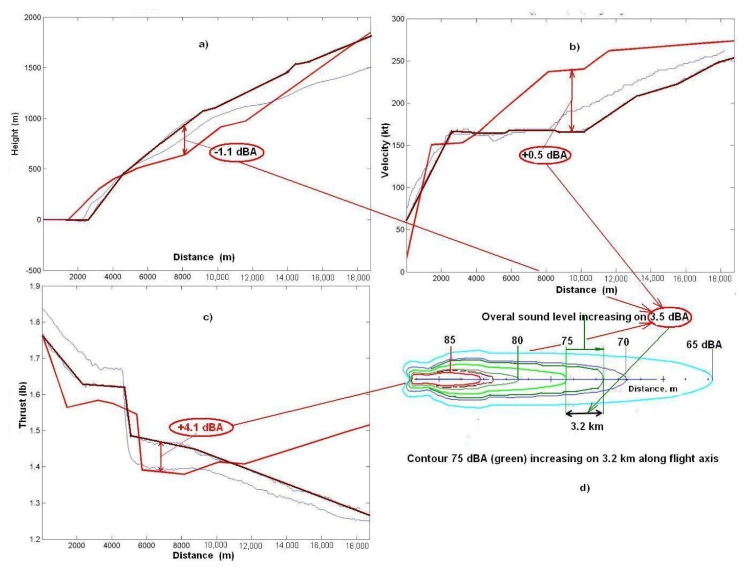
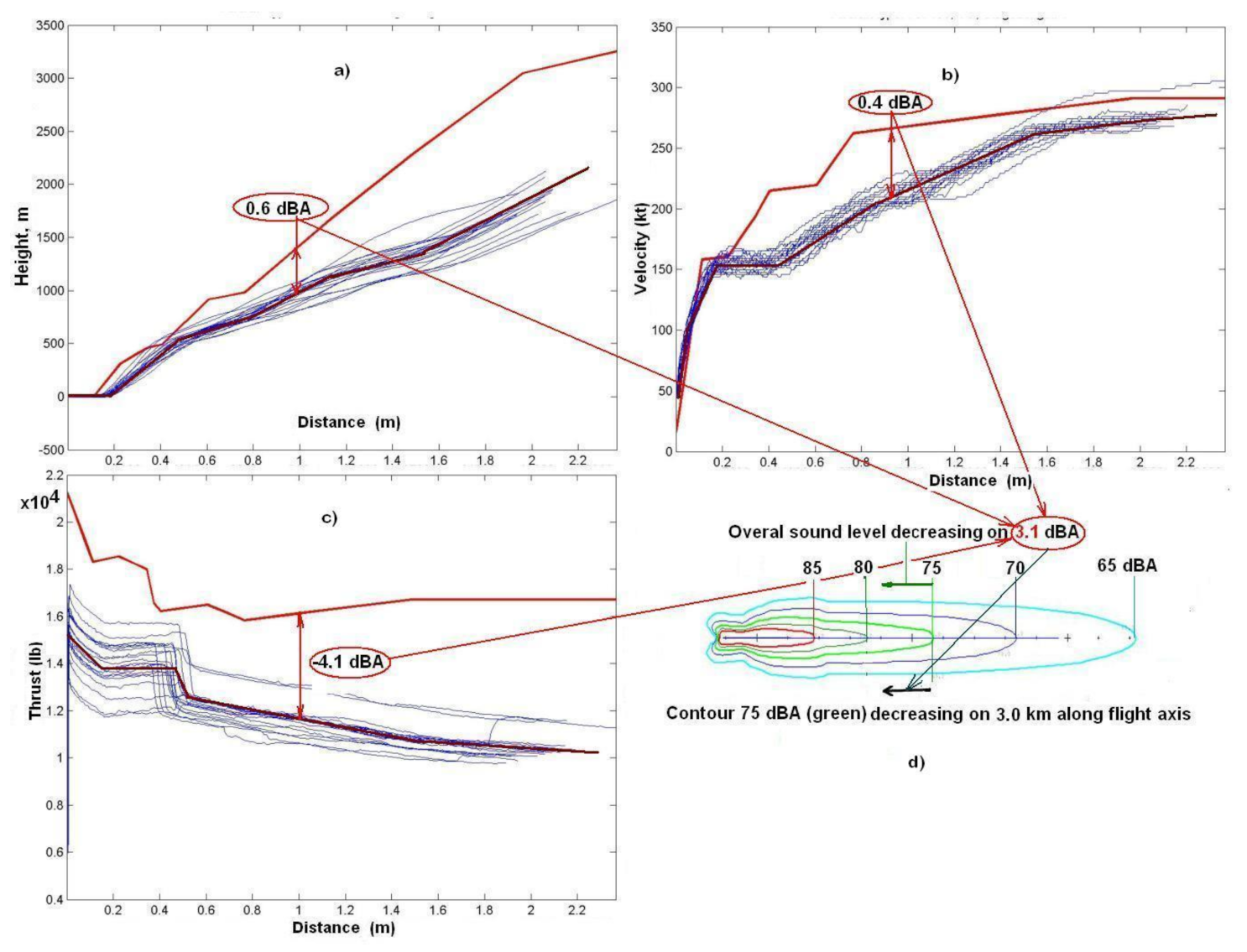
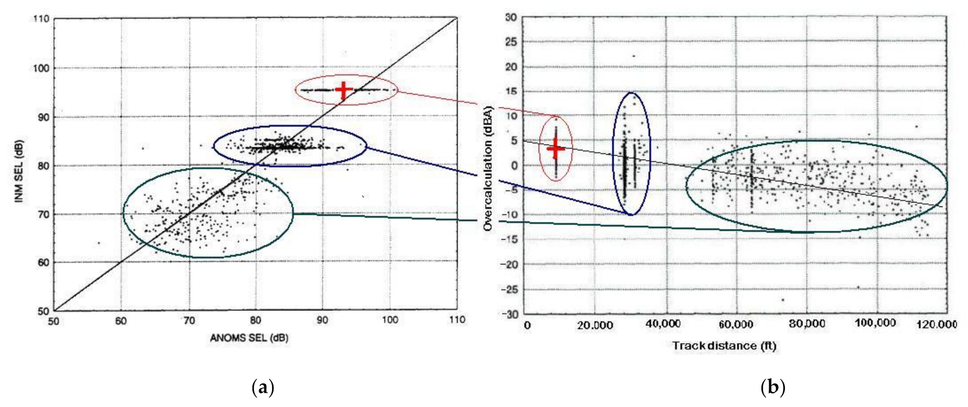
In Figure 8 the data for aircraft departure flight path are shown. To look at the flight speed (bottom figure), it should be found that operational speeds (blue) vary along the take-off/climbing stage of the flight path and usually are less than balanced values (red). Appropriate operational thrusts are much less also (right figure), but both of them—speed and thrust—are located in safe diapason, these data are the results of pilot operational qualification/safety culture and may be defined for every airport/airline/aircraft via statistical analysis. Fewer values for flight speed (right bottom in Figure 9) provide higher altitudes for the flight path in comparison with balanced solution, fewer values for thrust provides smaller altitudes for the flight path. By correction of the thrust with correspondent height and speed at climb out the contour for the LAmax = 75 dBA is predicted longer on 1.5 km comparing with balanced flight input data for standard atmosphere conditions as shown in Figure 11. The resulting difference between the real and balanced data may enhance the noise exposure in point and footprint like shown in Figure 11 (the real contour for the LAmax = 75 dBA is predicted longer on 3.2 km comparing with balanced flight input data), and/or reduce–like shown in Figure 12 (the real contour for the LAmax = 75 dBA is predicted shorter on 2.9 km comparing with balanced flight input data). Underestimation of sound level, both at departure and arrival, as a function to track distance, is observed elsewhere for particular flight events, for example, as shown for US INM ver. 5.1 Figure 13 for aircraft type Boeing-737 in [26]. Close to runway overcalculation may be observed (Figure 13b). On average INM predictions are about 3–5 dB lower than measured values at high SEL (closer to runway) and till 10 dB lower at low SEL (far from the runway). Such a pattern is typical for most analyses made elsewhere. The main contribution to this is provided by the huge difference between the calculated balanced thrust of the engine and the thrust observed in real flight (Figure 11c and Figure 12c). Improvements for engine thrust calculations must provide essential contribution in more accurate SEL (and LAmax) assessment for separate flyover noise.
In particular, the results of the study of aircraft noise in operational conditions show significant differences in flight profile (dependence of flight altitude on the distance in the vertical plane), flight speed, and mode of engine operation from the values obtained when calculating the equation of balanced motion, which are the basis of integrated models such as INM (USA) and IsoBella (Ukrainian analog developed at National Aviation University).
3.6. Corrections for More Accurate Sound Level Assessment
If the calculation of noise levels for individual segments of the flight profile is inaccurate on 1 dBA, the noise contour for the normative value of the sound level LAma = 75 dBA is shifted by 1.5–2 km in the direction of flight (Figure 10). Comparisons with real measurements usually show the smaller calculated values of sound levels for single events in most of the cases. In our practice of the portable noise measurements (noise control points were chosen on distances up to 2 km from runway, few of them very close to the arrival/departure nominal route and beneath the flight path, some of them–up to 1 km aside of it, aircraft fleet consists of short and middle distance airplanes like A-320, A-319, B-737, B-738, B-735, EMB-195, MD-83, DH-8, ATR-72, ATR-42, F-70, SAAB-2000, RJ-85) the diapason of changes at every point is quite huge, even for the same type of the aircraft and same flight mode, but their difference from the predictions is much greater. If the maximum levels were calculated between 75–92 dBA for these points, the maximum measured were between 78–99 dBA, the minimum–between 69–87 dBA, standard deviation between measured and calculated σ = 1.2–3.9 dBA [25].
For the terminals of the continuous noise monitoring system located within 2–4 km from the end of the runway, the averaged (arithmetic mean with standard deviation σcт = 0.3–1.0 dBA) measured values of LAmax were greater than those calculated by 0.8–1.2 dBA for different types of medium-haul aircraft (MD 81–90, Boeing 737-500−800), although in some cases differences for LAmax were observed up to 2–5 dBA (Figure 12 and Figure 13). Similarly, for the take-off/altitude phase along with flight segments that contribute to the sound level on certain monitors (ΔLAmax = 0.3–0.5 dBA, σcт = 0.2–0.5 dBA), the flight speed is usually observed to be lower than the balanced value by 20–50 m/s, and the actual operational thrust of the engines is observed both higher and lower than the balanced value, which generally causes a difference in sound levels ΔLAmax ± 4–5 dBA (Figure 11 and Figure 12). The noise circuit for LAmax 75 dBA (noise standard for the night according to the requirements of State Sanitary Rules [7]) for the takeoff of the aircraft type MD 81 increases along the flight axis more than 3 km in this case.
The method of aircraft trajectory segmentation takes into account the peculiarities of changes in flight parameters along with segments and their impact on sound level for the current segment. In particular, the linearized equation for estimating the angle of elevation along a rectilinear segment of the trajectory with a constant flight speed has the form:
where the coefficient k = 1.01 according to the methodology of the SAE-AIR-5662 [19] standard takes into account the increased climbing gradient due to headwinds with a speed wv ≈ 4.1 m/s, and the equivalent airspeed inherent in climbing, v = 82.3 m/s, Fn/δam—the available thrust of the engine, N—the number of engines, R—reverse aerodynamic quality, namely, the ratio of drag to lift coefficient CX/CУ for a given set of wing mechanization (flaps, slats, etc.), G is the total weight of the aircraft, δam = p/p0—the ratio of atmospheric pressure p at the point on the trajectory to the standard value of air pressure at sea level (p0 = 101,325 kPa).
In conditions of the actual operation, the value of the efficiency k is observed smaller, in a number of investigations its value for the type Boing-737 (−400–800) varied between 0.79–0.845; for type MD81-MD90—in the range of 0.93–0.985, but for MD81 in some cases the value k = 1.075. Accordingly, the calculated values of sound levels for departures are less than measured for the Boing-737-400 till ~3 dBA, for MD-81~3.5 dBA [27].
4. Ground Effect Correction
From an acoustic phenomenon only it is somewhat difficult to accept that if one is 400 m out to the side of an aircraft flight path and the aircraft is only several tens of meters above the ground surface or less, that one could expect an additional attenuation in the order of 10 dB (A) would result from ground effect—a calculation scheme for this phenomena is shown in Figure 14a. It is somewhat even more difficult to accept that, if one considers the same horizontal position but now increase the aircraft to few hundreds of meters above ground level that there would be excess attenuation across the ground in the order of 7 dB—these values are provided by the method incorporated in current standards and recommendations [1,13,17,19].
4.1. Homogeneous Atmosphere
If one is utilizing NPD measurements from the aircraft directly above the measurement position–directly how NPD data for the aircraft type should be evaluated [1,17], any reflection from the ground surface (Figure 15) would have already been incorporated in the results. The basic values of NPD-dependences are obtained during certification measurements (for flight path altitudes of 100–700 m over the point of noise measurement on a surface) for both takeoff and landing flight stages and if the microphone is installed at a height of 1.2 m above the ground surface, both direct and reflected sound rays are formed (in homogeneous atmosphere—as straight lines) and reach the microphone, the interference between them creates the ground effect even at the longitudinal plane (at points directly beneath the flight path, Figure 15c), not only for lateral to the trajectory points of noise control, Figure 15b. That is, the correction for “lateral attenuation of aircraft noise” is a methodologically incorrect definition, better to use “ground effect” for this phenomenon. However, this fact is currently not taken into account by the ICAO Doc 9911 methodology and the standard SAE AIR 5662 [19].
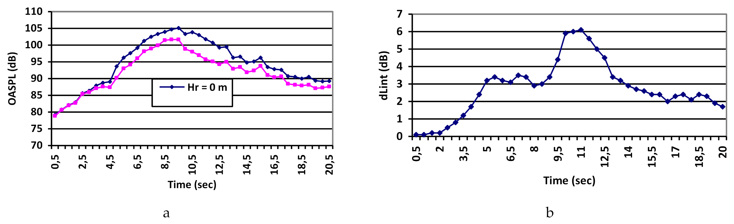
To increase the accuracy of single noise event calculation, it is necessary to calculate the correction for ground effect Λ(β,l) with higher accuracy and to use together with NPD-dependencies from the ANP database to determine the sound level of a particular segment of the flight path (Figure 14). Thus, for the take-off and descending flight profile at the microphone installation points beneath the trajectory, the interference effect is up to 6 dBA (Figure 16), which also introduces an error in the calculation of the maximum sound level under conditions of neglecting the ground effect in a plane of the flight path. If the ground effect was included in noise certification measurements thus the NPD-curves include it also and the direct usage of the model (2) in such case will provide the account of ground effect twice. For such case, the correction Λ(β,l) in model (2) must be the difference between ground effects just beneath the flight path and for (lateral) point aside flight path plane. The values of ground effect, as they are defined by the current ICAO Doc 9911 methodology, should be appropriate for usage with NPD-data with excluded ground effect only.
4.2. Inhomogeneous Atmosphere
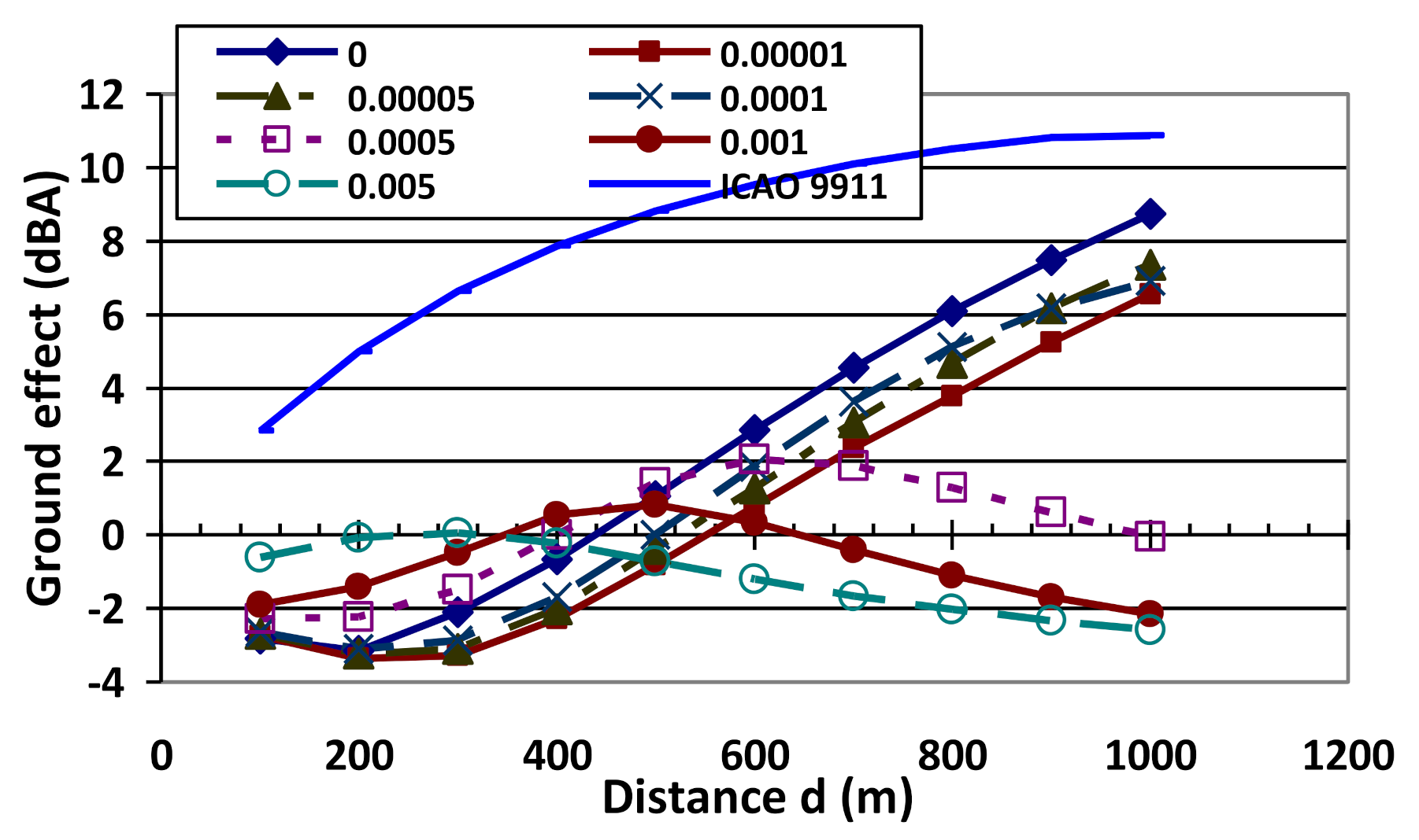
The last point of concern about the accuracy of ground effect assessment in any possible condition—how the wind speed gradient along the height over the ground surface and direction of the wind and also the temperature gradient influence the sound refraction between the aircraft (source) and point of noise measurement (receiver). With positive sound refraction (the sound speed increases with the altitude-sound waves are refracted down to the ground) ground effect may decrease, with negative (the average sound speed is decreasing with altitude, typically at daytime)—increase, in both cases the influence of sound incidence angle change will be most essential for total ground effect change. The influence of sound rays refraction on the ground effect was studied and it is shown in Figure 17 for sound speed gradient change in a range 0–0.005 s−1, it can be seen that for its positive value the ground effect decreases with increasing gradient: within the influence of the temperature gradient (a = 0.00001–0.0005 m−1) by 1–2 dBA, in the presence of wind (a = 0.001–0.005 m−1) downwards the propagation of sound, the effect may be at the level of its neglecting.
Figure 18 show a comparison of estimated from four airport’s short-term measurements of lateral attenuation of ground-to-ground (LA/GTG) sound propagation (source of noise is located on the ground, as a receiver microphone) with the calculated values of ground attenuation for NOITRA model with (a > 0) and without refraction (a = 0) and for equation from SAE AIR5662 [28]: for wind conditions “Upwind”, “Calm” and “Downwind”, respectively. The measurements were done similarly to noise trials at Figure 17—by microphones at Standard height 1.2 m and close to surface ~0.0 m, where interference effect or ground attenuation was defined by the difference between the measured values. SAE AIR5662 [19] does not include 1.5 dB of engine installation effects for airplanes with wing-mounted jet engines. The measured data for ground attenuation are located between the “Upwind” and “Downwind” calculation curves from [29], closely to “Calm” curve, which provides smaller values in comparison with current ICAO Doc 9911 [1].
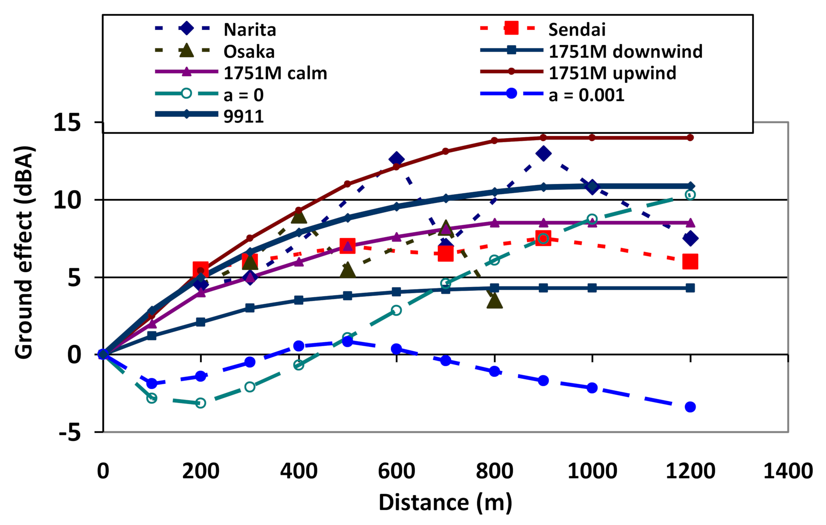
Figure 19 shows a comparison of the Air-to-Ground (ATG) component of lateral attenuation by using data of long-term noise monitoring at Narita airport from 50 selected stations located beneath and beside the straight flight route of the aircraft take-off. The shown in Figure 20 1751M-data (red line) were calculated with the modified reformulation of AIR 1751A [18] in accordance with proposed equations in [29].
Instead of constant 1.089 in the definition of distance factor Γ(λ) in [1,13,17] the term of G0(Vw, Tg) was introduced, it expresses a contribution of vector wind Vw using a sigmoid function and the second term considers the effect of temperature gradient Tg using a product of two sigmoid functions of respectively temperature gradient and vector wind [29,30]:
and Λ(β) is long-range air-to-ground lateral attenuation given by
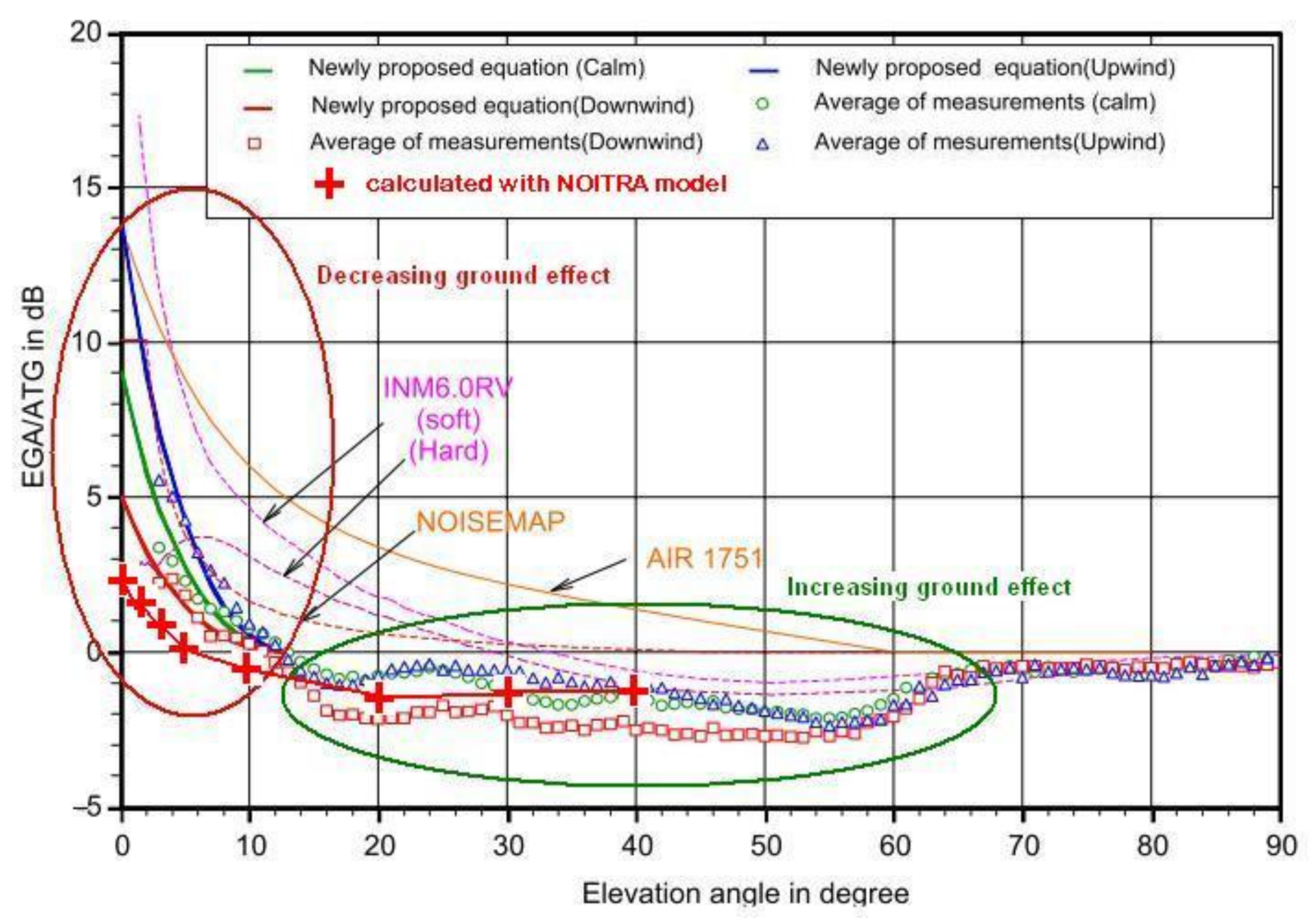
Both Figure 18 and Figure 19 show clearly that comprehensive measurements of the ground effect including meteorological effects on aircraft noise propagation aside of flight path, which were made with analysis of long-term observations of unattended noise monitoring of aircraft flyover noise around the airports, mostly at Narita Airport [28]. The results were divided into 3 classes of wind conditions, which are highly influencing sound refraction, but the observed meteorological conditions include the changes of seasons, temperature and humidity, wind and cloud in fact [28]. The calculated data with NOITRA model for calm conditions and averaged spectral class of the aeroplane noise at arrivals, also shown in Figure 19, confirm that ground effect in dependence to elevation angle changes dramatically from attenuation at quite small angles to amplifying effect at bigger elevation angles, which are in good correspondence with measurement results [28,29,30].
4.3. Inhomogeneous Atmosphere Influence on NPD-Data
The vertical gradient of the temperature exists always, for the standard atmosphere it is negative −6.5 °C/km. The study of the influence of the atmospheric state was performed to assess the NPD-data in dependence on temperature, pressure, humidity, which differ from the values of the standard atmosphere at sea level and along the altitude. In a homogeneous (non-refracting) atmosphere with changes in temperature and humidity (they have the greatest effect on the value of atmospheric sound absorption) within temperature −30 °C < t < +30 °C and humidity 1% < h < 85% of the values of sound exposure levels may differ from the ANP-data (which were defined for t = 25 °C and h = 70%) within diapason between −10 dBA and +15 dBA (larger deviations are observed for very dry air) for different aircraft spectral classes (used in current ANP database) in the flight modes of arrival and departure.
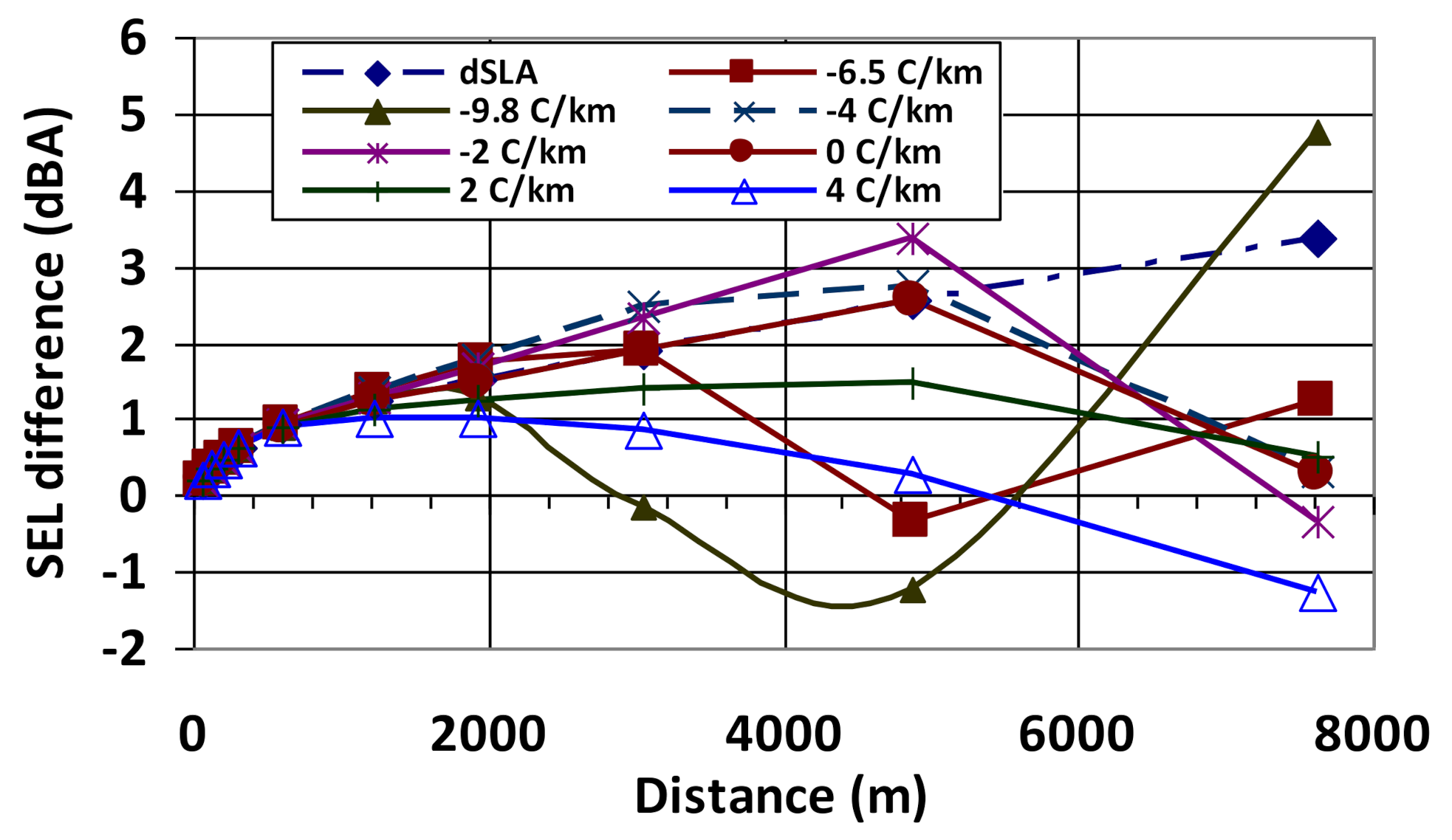
Under conditions of the inhomogeneous atmosphere, the influence of different profiles of temperature, pressure, humidity with altitude on the values of NPD-data for different spectral classes from the ANP database: for conditions of the standard atmosphere (GOST 4401-81) with a vertical temperature gradient −6.5 °C/km and the dependence of atmospheric sound absorption in accordance with GOST 31295.2-2005 (ISO 9613/2), the calculated values differ from the tabular ones on average up to ±2 dBA (Figure 20), their difference from other possible vertical temperature gradients in the atmosphere is insignificant. Influence of changes in the vertical humidity profile (in the range of 30–85% on the ground surface and up to 1% at the height of the maximum distance used in ANP database) from the values of GOST 31295.2-2005 and with constant temperature along the height over the ground surface—within ±1 dBA.
The dependencies “noise-power-distance” or NPD-dependence are decisive in the sound levels calculation, both for the single flight noise events and flight scenarios at the airport. In the current ANP database, their tabular values are given for the type of engine installed on aircraft, although for modern aircraft the contribution of aerodynamic noise produced by airflow around the wing and its mechanization is also significant, especially during the arrival stages of flight, where the engine operation mode is close to idle and the flaps and slats of the wing and gear are in a deflected position.
For aircraft with turbojet engines with high by-pass degrees (men > 10), the contribution of airframe noise is significant even at the departure flight of the aircraft. Therefore, neglecting the contribution of airframe noise today also significantly affects the accuracy of sound level calculations for both takeoff and landing. For A-320 and Boeing-737 aircraft of various modifications, the noise exposure from engines during aircraft arrival is ~10 dBA lower than the airframe noise exposure, so the study of aircraft noise, especially during arrival stages, should be used as the aerodynamic configuration of the aircraft-engine mode-distance or NAPD-dependence.
According to the improved integrated model for calculating noise from the aircraft in flight, the sound level generated by a separate segment of the flight path Lmax, seg, without any obstacle along the sound propagation path should be described by the formula:
the contribution to the sound exposure level LAE from each flight path segment is calculated by the formula:
where Lmax(P,A,d) and LE∞(P,A,d) are the values of sound levels from a particular segment of the flight path, which is determined based on the interpolation of NAPD tabular data (instead of NPD-data in Equation (2)) for the actual values of thrust or engine power P, aerodynamic configuration A and distance d. Other corrections in Equations (7) and (8) are the same as in the current model for aircraft noise calculation (2).
5. Discussion
The Noise-Power-Distance-relationship is a basic concept to calculate aircraft noise contours for air traffic in the airport nowadays. Current ICAO [1] and ECAC [13] recommendations, such as the complementarily standards [17,18,19], provide necessary accuracy for the calculation of equivalent levels and noise indices for the traffic scenario on their basis. Separate flyover noise events are still assessed with poor accuracy, never mind the requirements to operate with sound levels SEL and LAmax in a number of noise management tasks are very high.
Two main subjects of model improvements are discussed in the article—the difference between flight parameters in real operation and their values defined from solving a balanced system of aircraft movement. Statistical preparation of the data, observed in operation at the airport under consideration, provides more accurate values for flight thrust and velocity. The statistical values for coefficient k in Formula (4) from real operation allow to use more accurately the NPD-data and to cover the difference up to 5 dBA between calculated and measured sound levels under the flight paths.
Second important observation—how is influencing on calculated results the principal assumption of the method [1,7,8,9,10,11,12,13,14,15,16,17,18,19] about homogeneous atmosphere conditions. At the first stage for every compared integral model [2,3,4,5,6], the aircraft flight parameters are assessed for conditions with changed atmosphere parameters (air pressure, temperature, and humidity) along with the altitude. At the second stage, the noise levels are assessed for conditions of the homogeneous atmosphere, which is looking like methodological violation from one side, and from another side—new inaccuracy is produced in sound level assessment. If to look in Figure 15 for equal values of lateral distance at Figure 14a and vertical distance at Figure 15b the equal NPD-data should be used, it is appropriate with basic assumption. In real atmosphere due to change with an altitude of the meteorological parameters the NPD-data in case of Figure 15a,b will be quite different due to the contribution of different conditions for sound refraction, sound absorption (in case of Figure 15a it may be concerned as constant per distance unit, in case of Figure 14b the calculated influence is shown in Figure 20) and sound attenuation due to ground effect as shown in Figure 17, Figure 18 and Figure 19. The calculation accuracy may be improved till 5 dBA for separate flyover noise events by consideration of inhomogeneous conditions for sound propagation in the assessment of NPD-data and ground effect.
The ground effect itself should be considered as existing just beneath the flight path, so the “lateral attenuation” effect is methodically wrong. For future editions of the recommendations and standards [1,13,17,18,19], the term “ground effect” is looking enough.
For newish types of aircraft or their various modifications, especially with high by-pass engines in power plants (by-pass ratio till 10–12), the noise exposure from engines during aircraft arrival may be lower up to 10 dBA in comparison with airframe noise exposure. The current study of aircraft flyover noise exposure, especially during arrival stages, recommends using an aerodynamic configuration in basic noise-power-distance table data–namely NAPD-data. This new approach is not considered in detail in this article but will be a principal issue in near future.
6. Conclusions
The improvement of the integral noise model to calculate the sound exposure level LAE and maximum sound level LAmax for a single flight noise event according to the requirements to their accuracy may be achieved only with improvements of all basic elements of the current ICAO Doc 9911 [1] guidance. The main element of the model is the “noise-power-distance” dependence (NPD-dependence), which is recommended by the ICAO Doc 9911 and the Standard [17], should be replaced on “noise-power-airframe-distance”-dependence (NPAD-dependence), including the contribution of airframe noise dependent from various possible aerodynamic configurations. The always measured deviations of flight parameters from their balanced values (means the values, which are the solution of the system of equation for balanced motion) and real parameters of the state of atmosphere also contribute to the current inaccuracy of the single flight noise event assessment. The error in estimating the sound levels from the individual segments of the trajectories during departure after take-off and arrival before landing may be reduced on 5–10 dBA.
The model for estimating the ground effect (interference of direct and reflected from ground surface sound rays) should be improved in comparison with its current model of the ICAO Doc 9911 [1], which is overestimating the effect and inappropriate for the types of aircraft in use today. This may reduce the error by 4–6 dBA when calculating the sound levels LAmax and LAE to assess a single flight noise event by removing the contribution of the interference effect from NPD-dependencies and taking into account the correction for each spectral class of aircraft (turbojet, turbofan, turboprop/propeller) for two types of sound reflection surface–acoustically soft and hard.
The data from different research were reviewed in an article to show the similar view of other experts on similar effects of sound propagation first of all. So the improvement of the method [1,13,17,18,19] is of the highest importance in near future and the ways for this are assessed and recommended.
Author Contributions
Conceptualization, O.Z.; methodology, O.Z.; software, O.Z. and L.L.; validation, O.Z. and L.L.; formal analysis, O.Z.; investigation, O.Z. and L.L.; resources, O.Z. and L.L.; data curation, O.Z. and L.L.; writing—original draft preparation, O.Z. and L.L.; writing—review and editing, O.Z.; visualization, O.Z. and L.L.; supervision, O.Z.; project administration, O.Z. All authors have read and agreed to the published version of the manuscript.
Funding
This research received no external funding.
Institutional Review Board Statement
Not Applicable.
Informed Consent Statement
Not Applicable.
Data Availability Statement
Not Applicable.
Acknowledgments
Acknowledgement to EC ANIMA (Aviation Noise Impact Management through Novel Approaches) project No. H2020-MG-2017-SingleStage-INEA-769627.
Conflicts of Interest
The authors declare no conflict of interest.
References
- Recommended Method for Computing Noise Contours Around Airports, 2nd ed.; ICAO Doc 9911; ICAO: Montreal, QC, Canada, 2018; ISBN 978-92-9258-360.
- Volpe, J.A. Integrated Noise Model (INM) Version 7.0 Technical Manual; FAA-AEE-100; Office of Environment and Energy, the U.S. Department of Transportation, National Transportation Systems Center (Volpe Center) Acoustics Facility: Cambridge, MA, USA; The ATAC Corporation: Sunnyvale, CA, USA, 2015; p. 211, FAA-AEE-08-01. Available online: https://www.faa.gov/about/office_org/headquarters_offices/apl/research/models/inm_model/inm7_0c/media/INM_7.0_Technical_Manual.pdf (accessed on 2 April 2021).
- Ollerhead, J.B.; Rhodes, D.P.; Viinikainen, M.S.; Monkman, D.J.; Woodley, A.C. The UK Civil Aircraft Noise Contour Model ANCON: Improvements in Version 2; R&D Report 9842; National Air Traffic Services Ltd: Kingsway, London, 1999; p. 41. ISBN 0-86039-924-9. Available online: www.caa.co.uk (accessed on 2 April 2021).
- STAPES. SysTem for AirPort Noise Exposure Studies; Final Report; EUROCONTROL: Bruxelles, Belgium, 2009; p. 111, TREN/05/ST/F2/36-2/2007-3/S07.77778. [Google Scholar]
- Study on Current and Future Aircraft Noise Exposure at and around Community Airports; Final Report PAN012-4-0; MPD Group Limited: London, UK, 2003; p. 99. Available online: https://ec.europa.eu/transport/modes/air/studies/environment_en (accessed on 2 April 2021).
- Zaporozhets, O. Aircraft Noise Models for Assessment of Noise around Airports—Improvements and Limitations; ICAO Environmental Report; ICAO: Montreal, QC, Canada, 2016; pp. 50–55. Available online: https://www.icao.int/environmental-protection/Documents/EnvironmentalReports/2016/ENVReport2016_pg50-55.pdf (accessed on 2 April 2021).
- DSP 173-96. State sanitary rules of planning and development of settlements [ДСП 173-96. Державні санітарні правила планування та забудoви населених пунктів]; No. 379/1404;1996; Ministry of Justice of Ukraine: Kyiv, Ukraine, 2008; Available online: https://dnaop.com/html/2375/doc-%D0%94%D0%A1%D0%9F_173-96 (accessed on 2 April 2021). (In Ukrainian)
- Aviation Rules of Ukraine Requirements to the Aerodrome Operator Regarding the Spatial Zoning of the Area around the Airport from the Conditions of Exposure to Aviation Noise; No. 381 26; Civil Aviation Authority of Ukraine: Kyiv, Ukraine, 2019. Available online: https://zakon.rada.gov.ua/laws/show/z0461-19 (accessed on 2 April 2021). (In Ukrainian)
- ISO/CD 20906. Acoustics—Unattended Monitoring of Aircraft Sound in the Vicinity of Airports; ISO Central Secretariat, Vernier: Geneva, Switzerland, 2009; p. 36. [Google Scholar]
- Zaporozhets, O. AIRCRAFTNOISE: Assessment, Prediction and Control; Zaporozhets, O., Tokarev, V., Attenborough, K., Eds.; CRC Press Reference: Abingdon, UK, 2017; p. 420. ISBN 9781138073029. [Google Scholar]
- Zaporozhets, O.; Tokarev, V. Aircraft noise modelling for environmental assessment around airports. Appl. Acoust. 1998, 55, 99–127. [Google Scholar] [CrossRef]
- ICAO Technical Manual for Environment Specified the Usage of Methods for Aircraft Noise Certification; Doc. 9501 AN; ICAO: Montreal, QC, Canada, 1995.
- Report on Standard Method of Computing Noise Contours around Civil Airports, 4th ed; ECAC. CEAC Doc 29; ECAC: Cédex, France, 2016; Volumes 1–3, Available online: https://www.ecac-ceac.org/ecac-documents?p_p_id=101&p_p_lifecycle=0&p_p_state=maximized&p_p_mode=view&_101_struts_action=%2Fasset_publisher%2Fview_content&_101_assetEntryId=245876&_101_type=content&_101_urlTitle=ecac-directors-general-endorse-the-new-edition-of-ecac-doc-29-on-standard-method-of-computing-noise-contours-around-civil-airports (accessed on 2 April 2021).
- ICAO Standard and Recommended Practice. Environmental Protection. Annex 16 to the Convention on International Civil Aviation. Aircraft Noise, 8th ed.; ICAO: Montreal, QC, Canada, 2017; Volume 1. [Google Scholar]
- Recommendations for the Establishment of Zones of Restriction of Residential Development in the Vicinity of Civil Aviation Airports from Noise Conditions [Рекoмендациипoустанoвлениюзoнoграниченияжилoйзастрoйкивoкрестнoстяхаэрoпoртoвгражданскoйавиацииизуслoвийшума—М.: НИИСФ, ГoсНИИГА, МНИИгигиены]; State Research Institute of Civil Aviation: Moscow, Russia, 1987. (In Russian)
- Recommended Method for Computing Noise Contours Around Airports; Circular 205 AN/1/25; ICAO: Montreal, QC, Canada, 1988.
- SAE AIR 1845A. Procedure for the Calculation of Airplane Noise in the Vicinity of Airports; SAE Standard; SAE International: Warrendale, PA, USA, 2012. [Google Scholar]
- SAE AIR 1751A. Prediction Method for Lateral Attenuation of Airplane Noise During Takeoff and Landing; SAE Standard; SAE International: Warrendale, PA, USA, 2012. [Google Scholar]
- SAE AIR 5662. Method for Predicting Lateral Attenuation of Airplane Noise; SAE Standard; SAE International: Warrendale, PA, USA, 2019. [Google Scholar]
- Fleming, G.G.; Senzig, D.A.; McCurdy, D.A.; Roof, C.J.; Rapoza, A.S. Engine Installation Effccts of Four Civil Transport Airplancs: Wallops Flight Facility Study; NASA/TM-2003-212433; VA 33681-3199; NASA Langley Research Center: Hampton, VA, USA, 2003; p. 69. [Google Scholar]
- Idar, L.; Granøien, N. Comparison of INM Profiles and Measured Flight Profiles at GARDERMOEN; SINTEF Report STF40 A02032; SINTEF Telecom and Informatics: Trondheim, Norway, 2002. [Google Scholar]
- ADS-B Implementation and Operations Guidance Document, 11th ed.; ICAO APAC: Bangkok, Thailand, 2018.
- Measurement and Assessment of Aircraft Sound; Beuth Verlag GmbH: Berlin, Germany, 2011; DIN 45643; Available online: https://www.beuth.de/de/norm/din-45643/136846081 (accessed on 2 April 2021).
- Plotkin, K.J. Analysis of Acoustic Modeling and Sound Propagation in Aircraft Noise Prediction. NASA/CR-2006-214503 Wyle Lab. 2006. [Google Scholar]
- Zaporozhets, O.; Kartyshev, O. Aircraft noise assessment in the vicinity of airports with different descriptors. In Proceedings of the Aircraft Noise and Emissions Reduction Symposium (ANERS-2011), Marseille, France, 25–27 October 2011; Available online: www.aners2011.com; http://airportnoiselaw.org/symposia.html (accessed on 2 April 2021).
- Forsyth, D.W.; Gulding, J.; DiPardo, J. Review of Integrated Noise Model (INM) Equations and Processes. NASA/CR-2003-212414 2003, 56. [Google Scholar]
- Zaporozhets, O.; Levchenko, L. Detailed flight operation data for accurate aircraft noise assessment. In Proceedings of the World Aviation Congress, Kyiv, Ukraine, 10–12 October 2018; Available online: http://conference.nau.edu.ua/index.php/Congress/Congress2018/paper/viewFile/5402/4299 (accessed on 2 April 2021).
- Shinohara, N.; Nakazawa, T. Verification of comparison between measurement and prediction results of lateral attenuation derived from equations used in aircraft noise prediction. In Proceedings of the INTER-NOISE and NOISE-CON Congress and Conference Proceedings, Madrid, Spain, 16–19 June 2019; p. 10, Paper No. 2057. [Google Scholar]
- Yamada, I.; Shinohara, N. Developing an aircraft noise prediction model considering ground effects dependent on meteorological conditions. In Proceedings of the INTER-NOISE and NOISE-CON Congress and Conference Proceedings, Honolulu, HI, USA, 3–6 December 2006. [Google Scholar]
- Shinohara, N.; Makino, K.; Tsukioka, H.; Yoshioka, H.; Yamada, I. Evaluation of excess ground attenuation considering meteorological conditions. In Proceedings of the INTER-NOISE and NOISE-CON Congress and Conference Proceedings, Prague, Czech Republic, 22–25 August 2004. [Google Scholar]
- Granøien, I.L.N.; Randeberg, R.T. Corrective measures for aircraft noise models, new algorithms for lateral attenuation. In Proceedings of the Joint Baltic-Nordic Acoustics Meeting, Mariehamn, Åland, 8–10 June 2004; p. 9, Paper 041. [Google Scholar]
Figure 1.
Noise footprint for the departure of the aircraft with two certification points inside: 1—sideline point at take-off; 2—flight axis point at take-off and initial climbing.
Figure 1.
Noise footprint for the departure of the aircraft with two certification points inside: 1—sideline point at take-off; 2—flight axis point at take-off and initial climbing.

Figure 2.
Dependence of noise level LAmax with distance for departure (blue) and arrival (magenta) flight paths [15]: (a) longitudinal dependence, the departure from runway end of roll during take-off; arrival from the runway end of landing; (b) lateral dependence.
Figure 2.
Dependence of noise level LAmax with distance for departure (blue) and arrival (magenta) flight paths [15]: (a) longitudinal dependence, the departure from runway end of roll during take-off; arrival from the runway end of landing; (b) lateral dependence.

Figure 3.
Aircraft engine directivity pattern. Where: (a) Turbojet and turbofan with small by-pass ratio engine [15]; (b) Propeller and turboprop engine [15]; (c) Comparison with ICAO Doc 9911 for the backward direction.

Figure 4.
Measured lateral attenuation versus elevation angle and versus SAE prediction [21]: installation effect contribution for the airplane with engines in the tail is higher than or under the wing.
Figure 4.
Measured lateral attenuation versus elevation angle and versus SAE prediction [21]: installation effect contribution for the airplane with engines in the tail is higher than or under the wing.

Figure 5.
Construction of noise restriction zones taking into account the possible deviation of aircraft from standard route [15]: (a) the corridors for departure and arrival; (b) noise contours: 1—for the nominal route; 2—with an account of possible deviation of aircraft from the nominal route.
Figure 5.
Construction of noise restriction zones taking into account the possible deviation of aircraft from standard route [15]: (a) the corridors for departure and arrival; (b) noise contours: 1—for the nominal route; 2—with an account of possible deviation of aircraft from the nominal route.

Figure 6.
Comparison of measured and calculated noise contours for B-737 (a) and A-320 (b) aircraft during departure flight: blue crosses and dashed line are shown for locations where the LAmax was measured in airfield conditions; black contour–RF Acoustic Lab result of calculation; colored (85-red, 75-blue, 65-green) contours–US INM result of calculation [25].


Figure 7.
Flight profiles (height via distance) observed in operation (blue-colored) in comparison with balanced prediction (red-colored) [21]: (a)—arrival; (b)—departure.
Figure 7.
Flight profiles (height via distance) observed in operation (blue-colored) in comparison with balanced prediction (red-colored) [21]: (a)—arrival; (b)—departure.

Figure 8.
Balanced predictions for departure thrusts are much less than observed in operation thrusts. The data for the figure is used from [21].
Figure 8.
Balanced predictions for departure thrusts are much less than observed in operation thrusts. The data for the figure is used from [21].

Figure 9.
Comparison between observed in operation (blue) velocities and thrusts and predicted balanced values (red). The data for the figure is from [21].
Figure 9.
Comparison between observed in operation (blue) velocities and thrusts and predicted balanced values (red). The data for the figure is from [21].

Figure 10.
IsoBella results for B-737-400 noise contours (approach/landing and take-off/climbing): over—with input data for flight parameters observed in operation and below—for balanced input data for flight parameters.
Figure 10.
IsoBella results for B-737-400 noise contours (approach/landing and take-off/climbing): over—with input data for flight parameters observed in operation and below—for balanced input data for flight parameters.

Figure 11.
Contributions of the inaccuracy in calculation of the flight profile parameters in an overall calculation accuracy of the sound levels and noise contours for MD-81 departure. The flight data for the figure is used from [21]: (a)—flight path height contribution; (b)—flight path velocity contribution; (c)—flight path thrust contribution; (d)—overall sound level is rising on 3.5 dBA and noise contour 75 dBA increasing on 3.2 km along the axis of departure.

Figure 12.
Contributions of the inaccuracy in calculation of the flight profile parameters in an overall calculation accuracy of the sound levels and noise contours for B-734 takeoff. The flight data for the figure is used from [21]: (a)—flight path height contribution; (b)—flight path velocity contribution; (c)—flight path thrust contribution; (d)—overall contribution to sound level and noise contours.

Figure 13.
Comparison between measured and INM 5.1a calculated SEL for B-733 (combined from the figures, which are taken from [26]): (a)—correlation between the measured and calculated data; (b)—overcalculation as a function to track distance.
Figure 13.
Comparison between measured and INM 5.1a calculated SEL for B-733 (combined from the figures, which are taken from [26]): (a)—correlation between the measured and calculated data; (b)—overcalculation as a function to track distance.

Figure 14.
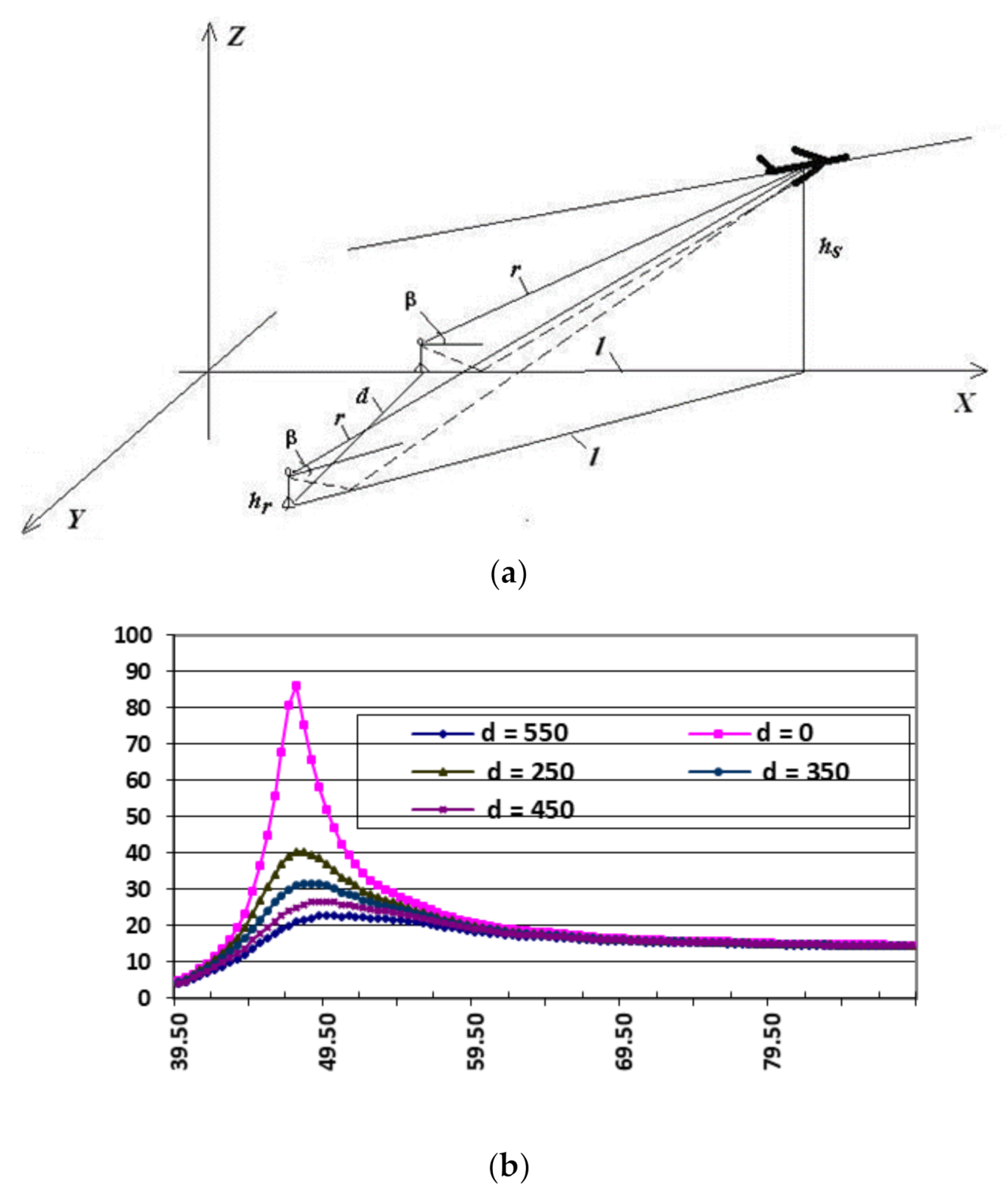
Elevation angle for point of noise measurement beneath and lateral to flight path: (a)—scheme to define the elevation angle β and distance l to the noise source; (b)—dependence of elevation angle β from the lateral distance d (in meters).
Figure 14.
Elevation angle for point of noise measurement beneath and lateral to flight path: (a)—scheme to define the elevation angle β and distance l to the noise source; (b)—dependence of elevation angle β from the lateral distance d (in meters).

Figure 15.
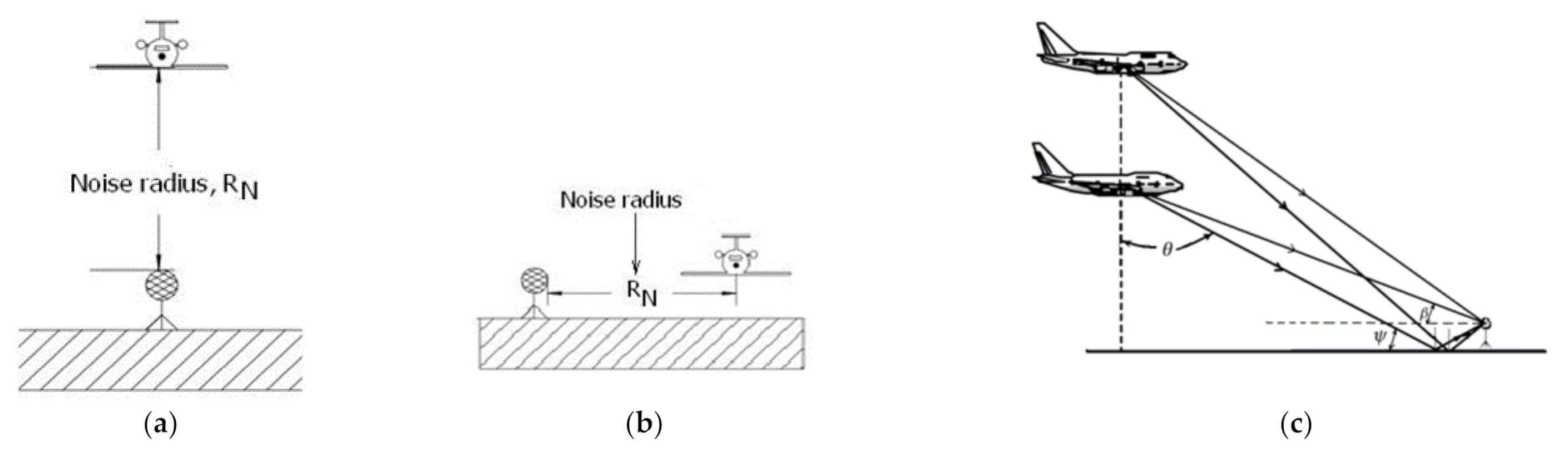
Elevation angle for point of noise measurement beneath (a) and lateral (b) to the flight path, and ahead of the airplane (c) in the vertical plane: β—the elevation angle, θ—incidence angle, ψ—grazing angle and distance R to the noise source.
Figure 15.
Elevation angle for point of noise measurement beneath (a) and lateral (b) to the flight path, and ahead of the airplane (c) in the vertical plane: β—the elevation angle, θ—incidence angle, ψ—grazing angle and distance R to the noise source.

Figure 16.
Sound interference effect (or ground effect) measured beneath the take-off/climbing trajectory: (a) overall sound pressure levels dependence with (for the microphone at height Hr = 1.2 m) and without (for the microphone at height Hr = 0.0 m) ground effect; (b) ground effect d Lint itself.

Figure 17.
Influence of the vertical gradient of the sound speed on ground effect (soft acoustic surface—grass cover) [27].
Figure 17.
Influence of the vertical gradient of the sound speed on ground effect (soft acoustic surface—grass cover) [27].

Figure 18.
Comparison of lateral attenuation of ground-to-ground (LA/GTG) at 4 airports in Japan [28] (small dash lines) with existing formulas from the standards [18,19] and refraction influence investigation with NOITRA (dash lines).

Figure 19.
Results of the average of estimated EGA/ATG respectively for the three wind conditions (upwind, calm, and downwind) [28] compared with EGA/ATG value from standards [18,19]: ground effect decreasing the overall sound level is observed for elevation angles β < 12°; for higher elevation angles (12° < β < 70°) the ground effect may increase the overall sound level at the point of noise control.

Figure 20.
Influence of the vertical gradient of atmospheric air temperature on the difference of the calculated data in comparison to tabular values of NPD-dependences [27].
Figure 20.
Influence of the vertical gradient of atmospheric air temperature on the difference of the calculated data in comparison to tabular values of NPD-dependences [27].


Table 1.
Simplified scheme of integrated aircraft noise model development in historical perspective.
Table 1.
Simplified scheme of integrated aircraft noise model development in historical perspective.
| Integrated Aircraft Noise Model Structure | Period | |||
|---|---|---|---|---|
| Source (Aircraft) Performances Model | Noise Performance Model | |||
| Lateral Distribution of the Flight Routes | Vertical Flight Path | Noise-Distance Relationship | Corrections | |
| Tracks and flight corridors from the Flight Chart | Flightpath for specific flight stage and aircraft group | Dependence of noise level with distance along flight axis | Lateral sound level change from longitudinal value along flight axis | 1970–1980s |
| Calculated flight path for specific flight stage and specific aircraft type | NPD-curves for the specific aircraft type (with specified engine type in power plant) | averaged for overall aircraft fleet corrections for engine installation effect, lateral effect, the directivity of noise propagation | 1990s | |
| Tracks and flight corridors from the Flight Chart + lateral distribution of the flight | Calculated flight path for specific flight stage and specific aircraft type in accordance with real meteorological parameters | NPD-curves for specific aircraft type with the possibility to recalculate them in accordance with real meteorological parameters and a spectral class of the aircraft | Corrections for engine installation effect for the tail and under the wing-mounted engines, the directivity of noise propagation for by-pass and propeller engines, lateral effect still general for overall fleet | 2000–2010s |
| Real tracks (from the airport radar data) | Real flight paths (from the airport radar data) | NPD-curves for specific aircraft type recalculated in accordance with real meteorological parameters and a spectral class of the aircraft | ||
| Real flight tracks (from the airport radar data or ADS-B data) | Real flight paths (from the airport radar data or ADS-B data) | Corrections for engine installation effect for the specific aircraft type, directivity of noise propagation, and ground (not lateral) effect for specific aircraft type or spectral class | 2010–2020s | |
| Real flight tracks and taxiing tracks (from the ADS-B data) | ||||
Publisher’s Note: MDPI stays neutral with regard to jurisdictional claims in published maps and institutional affiliations. |
© 2021 by the authors. Licensee MDPI, Basel, Switzerland. This article is an open access article distributed under the terms and conditions of the Creative Commons Attribution (CC BY) license (https://creativecommons.org/licenses/by/4.0/).
Share and Cite
MDPI and ACS Style
Zaporozhets, O.; Levchenko, L. Accuracy of Noise-Power-Distance Definition on Results of Single Aircraft Noise Event Calculation. Aerospace 2021, 8, 121. https://0-doi-org.brum.beds.ac.uk/10.3390/aerospace8050121
AMA Style
Zaporozhets O, Levchenko L. Accuracy of Noise-Power-Distance Definition on Results of Single Aircraft Noise Event Calculation. Aerospace. 2021; 8(5):121. https://0-doi-org.brum.beds.ac.uk/10.3390/aerospace8050121
Chicago/Turabian StyleZaporozhets, Oleksandr, and Larisa Levchenko. 2021. "Accuracy of Noise-Power-Distance Definition on Results of Single Aircraft Noise Event Calculation" Aerospace 8, no. 5: 121. https://0-doi-org.brum.beds.ac.uk/10.3390/aerospace8050121
Note that from the first issue of 2016, this journal uses article numbers instead of page numbers. See further details here.