An Explosion Based Algorithm to Solve the Optimization Problem in Quadcopter Control

Abstract

This paper presents an optimization algorithm named Random Explosion Algorithm (REA). The fundamental idea of this algorithm is based on a simple concept of the explosion of an object. This object is commonly known as a particle: when exploded, it will randomly disperse fragments around the particle within the explosion radius. The fragment that will be considered as a search agent will fill the local space and search that particular region for the best fitness solution. The proposed algorithm was tested on 23 benchmark test functions, and the results are validated by a comparative study with eight well-known algorithms, which are Particle Swarm Optimization (PSO), Artificial Bee Colony (ABC), Genetic Algorithm (GA), Differential Evolution (DE), Multi-Verse Optimizer (MVO), Moth Flame Optimizer (MFO), Firefly Algorithm (FA), and Sooty Tern Optimization Algorithm (STOA). After that, the algorithm was implemented and analyzed for a quadrotor control application. Similarly, a comparative study with the other algorithms stated was done. The findings reveal that the REA can yield very competitive results. It also shows that the convergence analysis has proved that the REA can converge more quickly toward the global optimum than the other metaheuristic algorithms. For the control application result, the REA controller can better track the desired reference input with shorter rise time and settling time, lower percentage overshoot, and minimal steady-state error and root mean square error (RMSE).

1. Introduction

Over the past few years, the popularity of metaheuristic optimization techniques to solve complex real-life problems has grown among researchers. The main reason for using metaheuristic optimization techniques is that they are relatively simple, flexible, non-transferable, and can avoid local stagnation [1]. The simplicity of the metaheuristic algorithms is derived from straightforward concepts that are typically inspired by physical phenomena, animal behavior, or evolutionary ideas. Flexibility refers to applying metaheuristic algorithms to different problems without any specific structural changes in its algorithm. Metaheuristic algorithms are easily applied to a variety of issues since they usually assume problems as black boxes. Most metaheuristic algorithms have mechanisms that are free of derivation.

In contrast to gradient-based optimization approaches, these algorithms stochastically optimize the problems. This optimization process begins with a random solution(s), and there is no need to calculate the derivative of the search spaces to find the optimum value. This makes metaheuristic algorithms highly suitable for real problems with expensive or unknown information on derivatives.

Compared to conventional optimization techniques, metaheuristic algorithms have a superior capability in avoiding local optima. Due to these algorithms’ stochastic nature, it is possible to prevent stagnation in local optima and search extensively throughout the search space. The real problem area is usually unknown and complicated with many local optima, so metaheuristic algorithms are excellent for optimizing these challenging problems.

Generally, metaheuristic algorithms can be divided into two categories: single-solution and multi-solution based. On a single-solution basis, the search process begins with one candidate solution improved throughout the iterations. Whereas multi-solution-based optimization was carried out using an initially random set of population solutions, these populations will be enhanced during the iterations. Multiple solutions (population) based optimization has some advantages over single-solution-based optimization [2]:

• There are multiple possible best solutions.
• There is information sharing between the multiple solutions that can assist each other to avoid local optima.
• Exploration in the search space of multiple solutions is more significant than a single solution.

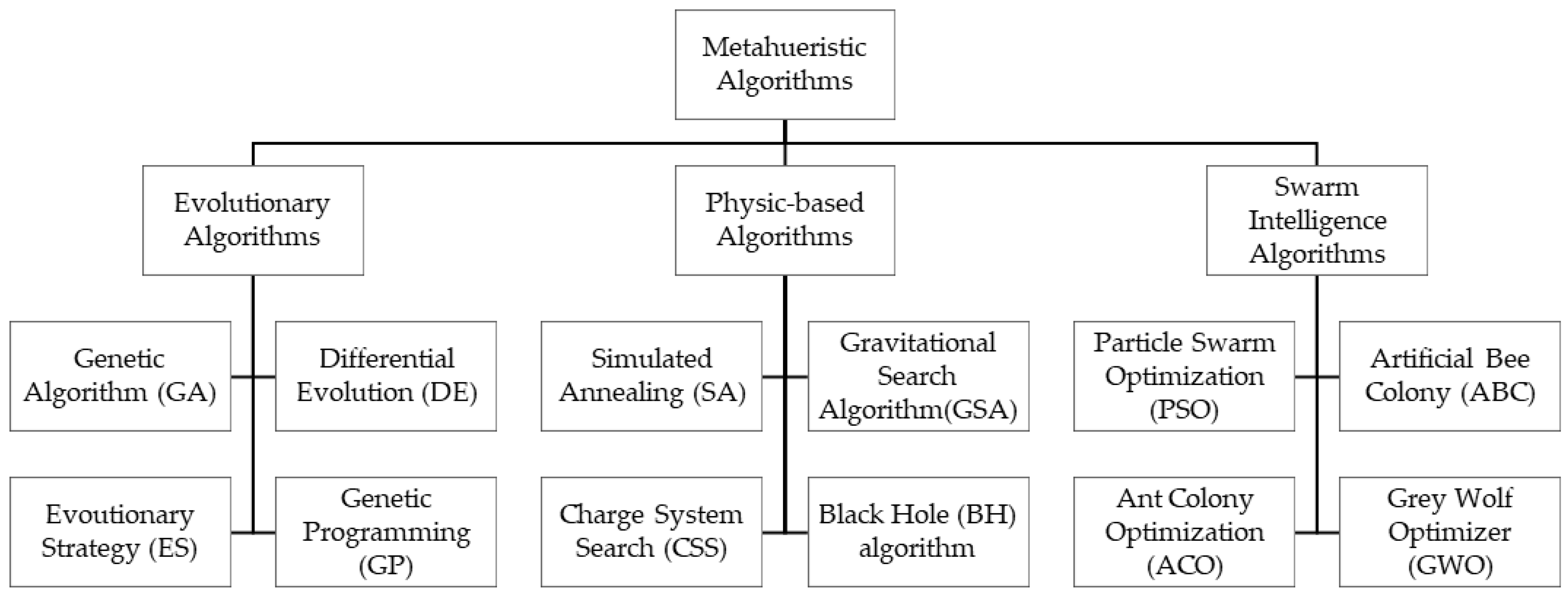
Furthermore, these metaheuristic algorithms can be classified further into three classes which are evolutionary-based, physical-based, and swarm-based methods [3], as shown in Figure 1. The first class is a generic population-based algorithm based on biological evolution, such as reproduction, mutation, recombination, and selection. This method often provides close-to-optimal solutions to all types of problems as it does not make any assumptions about the basic fitness landscape. Some of the popular metaheuristic algorithms based on the concept of evolution (EA) in nature are Genetic Algorithm (GA) [4], Differential Evolution (DE) [5], Evolution Strategy (ES) [6,7], Genetic Programming (GP) [8], and Biogeography-Based Optimizer (BBO) [9].

The second class of metaheuristic optimization is an algorithm based on physics. Such an optimization algorithm communicates with each search agent. The search agent moves across the search space according to the laws of physics, such as gravitational forces, electromagnetic forces, inertia, etc. These metaheuristic algorithms are Simulated Annealing (SA) [10], Gravitational Search Algorithm (GSA) [11], Black Hole (BH) algorithm [12], Ray Optimization (RO) algorithm [13], Big-Bang Big-Crunch (BBBC) [14], Central Force Optimization (CFO) [15], Charge System Search (CSS) [16], Small World Optimization Algorithm (SWOA) [17], Artificial Chemical Reaction Optimization Algorithm (ACROA) [18], Galaxy-based Search Algorithm (GbSA) [19], and Curve Space Optimization (CSO) [20].

The third class of metaheuristic optimization is swarm-based algorithms. These algorithms are based on social creatures’ collective behavior. Collective intelligence is based on the interaction of the swarms with each other and their environment. A few well-known Swarm Intelligence (SI) techniques are Particle Swarm Optimization (PSO) [21], Ant Colony Optimization (ACO) [22], Artificial Bee Colony (ABC) [23], Monkey Search (MS) [24], Cuckoo Search (CS) [25], Bat-inspired Algorithm (BA) [26], Dolphin Partner Optimization (DPO) [27], Firefly Algorithm (FA) [28], Bee Collecting Pollen Algorithm (BCPA) [29], and Marriage in Honey Bees Optimization Algorithm (MBO) [30].

There are two essential components in the metaheuristic algorithms that influence the solution’s efficiency and accuracy: the phases of exploration and exploitation [31,32]. The exploration phase ensures that the algorithm moves and explores the other promising regions in the search space. In contrast, the exploitation phase provides the search for the optimal solutions within the promising regions that have been achieved during the exploration phase [33]. The fine-tuning of these two components is crucial to obtain an optimal solution for the given optimization problems. However, due to the optimization problem’s stochastic nature, it is not easy to balance these two components. This motivates us to develop a new metaheuristic algorithm and to explore its ability to solve optimization problems.

In this paper, we will present a different metaheuristic algorithm for optimization problems. The main objective of this paper is to develop a robust algorithm. The term robust used in this paper is discussed based on the algorithm’s accuracy and consistency in finding the optimal solution for the benchmark function tested in several independent runs. For instance, as we know, a stochastic algorithm will not produce a similar result every time we run the algorithm. Thus, these algorithms will usually need to be run several times to see how many times a good result is achieved. Additionally, the average and standard deviation (typical statistical analysis) of the result can be obtained. This way, the result can be more convincing than a single run’s result. If the algorithm can provide a high consistency output result while maintaining its accuracy, then we can say that the algorithm is robust [34,35,36].

Hence, an algorithm based on the explosion of a set of initial particles that will produce a random scatter particle’s fragment around the initial particles within the explosion radius has been proposed, namely Random Explosion Algorithm (REA). According to the No-Free-Lunch (NFL) theorem [37], no algorithm can solve all the optimization problems alone, which means that a particular algorithm for a specific problem may show outstanding performance. Still, the same algorithm may give a poor performance on different problems. Therefore, it has led us to develop this robust algorithm.

The rest of this paper is organized as follows: Section 2 introduces the proposed algorithm’s concept. In Section 3, the benchmark test functions are presented. Section 4 will discuss the application of the algorithm for quadrotor control. In Section 5, the simulation results and discussion on the algorithm’s performance and the controllers and a comparative study with several other well-known existing algorithms are presented. Finally, a concluding remark is presented in Section 6.

2. Random Explosion Algorithm (REA)

In this section, the basic idea of the proposed REA algorithm is described in detail.

2.1. The Fundamental Concept

The concept of the proposed algorithm is based on the phenomena of an explosion. When a particle is exploded, it will produce numbers of fragments randomly scattered around the particle. Each particle’s fragments will be landed in a particular location called RF within the explosion radius, r_e. In our opinion, the particle’s fragments during the explosion are considered the search agent to search the local space around the particle.

After the first explosion occurs, we assume the fragment will become the new particle and continue to explode. This process will be repeated until it can no longer be exploded, in which whether the stopping criteria have been met or the explosion radius, r_e, is approaching zero. Based on whichever fragment, we chose the closest to the global best solution to select which fragments will become the next particle.

Since there is n-number of fragments produced during the explosion, the probability of finding the local optima or near local optima solution can be guaranteed. If we consider multiple particles, we can also assure that the global optimum can be found and avoid local optima’s stagnation. These particles 1, 2, 3, …, m, will search their own local space and update the best fitness so far based on the global optimum. This process will be repeated until all particles reach the only global optimum.

2.2. Design of the REA

Suppose that the initial position of the particles is defined in Equation (1) as $X_i^P$ is randomly generated within the lower and upper boundaries of search space and the current location of a particle is

$$X_i^P=X_d,\hspace{1em}\hspace{1em}i=1, 2, 3, \dots , m$$

(1)

where d indicates the dimension of the variable in the d dimensional search space. Then, for each particle, it will be exploded to produce randomly scattered fragments within the explosion radius, r_e, around the initial particle. The location of the fragments is determined as in Equation (2):

$$X_j^F=X_i^P+R_j^F,\hspace{1em}\hspace{1em}j=1, 2, 3, \dots , n$$

(2)

where $R_j^F$ is a uniformly distributed random number in the explosion radius, (−r_e, r_e).

Next, a selection of the new particle must be made to continue the explosion as the next generation. The best fragment in each group must replace the old particle that has been exploded before. A selection strategy based on the shortest distance between the current fragment in the current group and the global best solution is used to determine which fragment is the best. The following Equation (3) calculates the distance between the individual fragment and the global best solution, where GB is the global best solution.

$$D_j^i=\left|norm\left(GB-X_i^F\right)\right|$$

(3)

In this algorithm, the explosion radius plays an essential role in determining the performance of the algorithm. To make sure the agent is exploring the search space globally, a high value of explosion radius should be chosen at the beginning of the iteration and gradually decreasing until the end of the iteration. A higher value of the explosion radius will ensure the search agent explores the further search space (better exploration).

A lower value of the explosion radius lets the search agent exploit the potential region better (good exploitation). Furthermore, an appropriate number of fragments also must be chosen so that the chance of finding the best solution is higher. A simple technique to reduce the explosion radius, r_e, which is used in this work, is given in Equation (4), where c is a parameter constant, It is the current iteration, and MaxIt is the total number of iterations.

$$r_{e_{new}}=r_{e_{initial}}\times \exp \left(-c\times \frac{It}{MaxIt}\right)$$

(4)

2.3. Steps of Implementation of REA

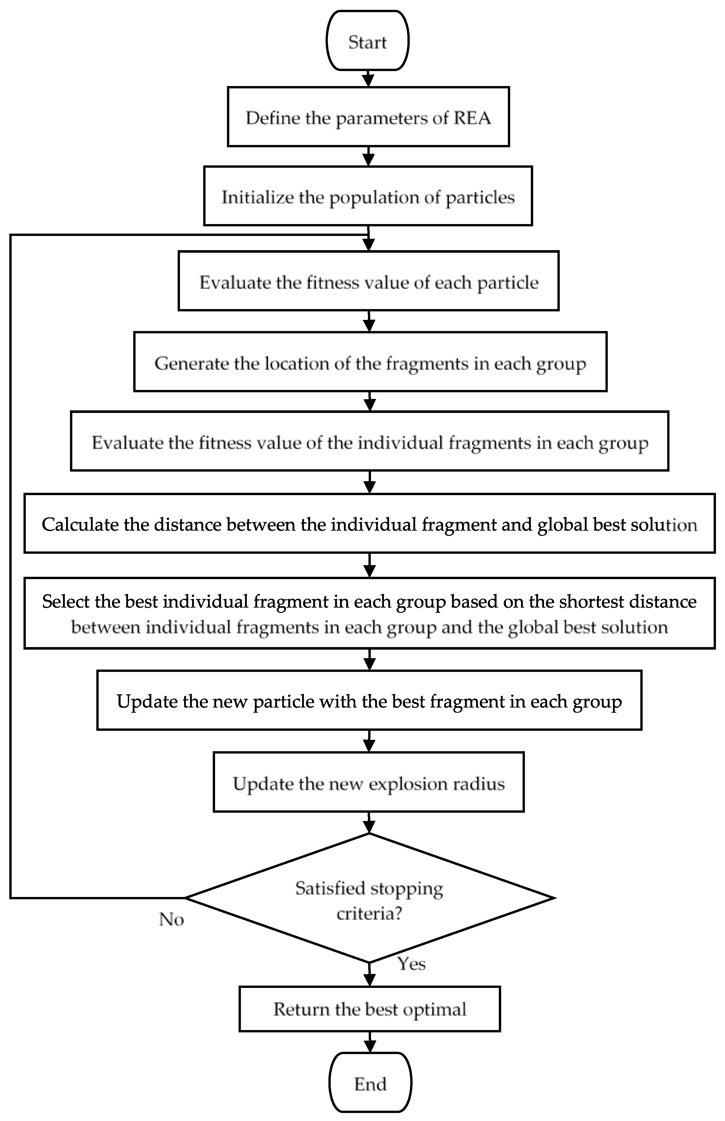
The flowchart of the proposed REA is presented in Figure 2 below.

The steps of implementation of REA are summarized as follows:

Step 1:

Define the parameters of REA (maximum iteration, number of particles, number of fragments, the radius of the explosion, c).

Step 2:

Initialize the particle population, $X_i^P$, within the lower and upper bound of the search space, where i = 1, 2, 3, …, m.

Step 3:

Evaluate the fitness value of each particle.

Step 4:

Explosion: Generate the location of n-number of random fragments, $X_j^F$, within the explosion radius, r_e, in each group (in the first explosion, an initial explosion radius is used; particle 1 will be group 1, particle 2 will be group 2, and so on).

Step 5:

Evaluate the fitness value of an individual fragment in each group.

Step 6:

Calculate the distance between individual fragments in each group and the global best solution.

Step 7:

Selection: Select the best fragment in each group which is the fragment that is nearest (minimum distance) to the global best solution.

Step 8:

Update the new particle with the best fragment in each group obtained in Step 7 to continue the next explosion.

Step 9:

Update the new explosion radius (explosion radius will be decreasing from the initial explosion radius to 0/~0).

Step 10:

If the stopping criterion is satisfied, then the algorithm will be stopped. Otherwise, return to Step 4.

Step 11:

Return the best optimal solution (after the stopping criteria are satisfied).

3. REA for the Benchmark Test Functions

Benchmark test functions are a group of functions that can test the performance and characteristics of any optimization algorithms for the various optimization problems, such as constrained/unconstrained, continuous/discrete, and unimodal/multimodal problems. For any new optimization algorithm developed, testing and evaluating the algorithm’s performance is very important. Therefore, the common practice to test how these new algorithms are performed compared to other algorithms is to test on the benchmark test functions. Furthermore, such benchmarking is also vital to gain a better understanding and greater insight into the pros and cons of the algorithms under-tested [38,39,40,41].

A total of 23 benchmark test functions are applied to the algorithm to demonstrate the algorithm’s efficiency. These benchmark test functions can generally be divided into three main categories, that are unimodal benchmark test functions [42], multimodal benchmark test functions [28] and fixed dimension benchmark test functions [28,42]. These benchmark functions are described in Appendix A in

Table A1. Unimodal benchmark function.

Function	Dim	Range	fmin
$F_1\left(x\right)={{\displaystyle \sum }}_{i=1}^n{x}_i^2$	10	(−100, 100)	0
$F_2\left(x\right)={{\displaystyle \sum }}_{i=1}^n\left|x_i\right|+{{\displaystyle \prod }}_{i=1}^n\left|x_i\right|$	10	(−10, 10)	0
$F_3\left(x\right)={{\displaystyle \sum }}_{i=1}^n{\left({{\displaystyle \sum }}_{j-1}^i{x}_j\right)}^2$	10	(−100, 100)	0
$F_4\left(x\right)=ma{x}_i\left\{\left|x_i\right|,1\le i\le n\right\}$	10	(−100, 100)	0
$F_5\left(x\right)={{\displaystyle \sum }}_{i=1}^{n-1}\left[100{\left(x_{i+1}-x_i^2\right)}^2+{\left(x_i-1\right)}^2\right]$	10	(−30, 30)	0
$F_6\left(x\right)={{\displaystyle \sum }}_{i=1}^n{\left(\left[x_i+0.5\right]\right)}^2$	10	(−100, 100)	0
$F_7\left(x\right)={{\displaystyle \sum }}_{i=1}^{n}i{x}_i^4+random\left(0, 1\right)$	10	(−1.28, 1.28)	0

,

Table A2. Multimodal benchmark function.

Function	Dim	Range	fmin
$F_8\left(x\right)={{\displaystyle \sum }}_{i=1}^n-x_i\sin \left(\sqrt{\left|x_i\right|}\right)$	10	(−500, 500)	−418.9829 × Dim
$F_9\left(x\right)={{\displaystyle \sum }}_{i=1}^n\left[x_i^2-10\cos \left(2\pi x_i\right)+10\right]$	10	(−5.12, 5.12)	0
$F_{10}\left(x\right)=-20\exp \left(-0.2\sqrt{\frac{1}{n}{{\displaystyle \sum }}_{i=1}^n{x}_i^2}\right)-\exp \left(\frac{1}{n}{{\displaystyle \sum }}_{i=1}^n\cos \left(2\pi x_i\right)\right)+20+e$	10	(−32, 32)	0
$F_{11}\left(x\right)=\frac{1}{4000}{{\displaystyle \sum }}_{i=1}^n{x}_i^2-{{\displaystyle \prod }}_{i=1}^n\cos \left(\frac{x_i}{\sqrt{i}}\right)+1$	10	(−600, 600)	0
$$\begin{gathered} F_{12}\left(x\right)=\frac{\pi }{n}\left\{10\sin \left(\pi y_1\right)+{{\displaystyle \sum }}_{i=1}^{n-1}{\left(y_i-1\right)}^2\left[1+10{\sin }^2\left(\pi y_{i+1}\right)\right]+{\left(y_n-1\right)}^2\right\} \\ +{{\displaystyle \sum }}_{i=1}^{n}u\left(x_i, 10, 100, 4\right)y_i=1+\frac{x_i+1}{4} \end{gathered}$$$u\left(x_i, a, k, m\right)=\{\begin{array}{c}k{\left(x_i-a\right)}^m x_i>a\\ 0 -a<x_i<a\\ k{\left(-x_i-a\right)}^m x_i<-a\end{array}$	10	(−50, 50)	0
$$\begin{gathered} F_{13}\left(x\right)=0.1\left\{{\sin }^2\left(3\pi x_1\right)+{{\displaystyle \sum }}_{i=1}^n{\left(x_i-1\right)}^2\left[1+{\sin }^2\left(3\pi x_i+1\right)\right] \\ +{\left(x_n-1\right)}^2\left[1+{\sin }^2\left(2\pi x_n\right)\right]\right\}+{{\displaystyle \sum }}_{i=1}^{n}u\left(x_i, 5, 100, 4\right) \end{gathered}$$	10	(−50, 50)	0
$F_{14}\left(x\right)=-{{\displaystyle \sum }}_{i=1}^n\sin \left(x_i\right)·{\left(\sin \left(\frac{i·x_i^2}{\pi }\right)\right)}^{2m}, m=10$	10	(0, π)	−4.687
$F_{15}\left(x\right)=\left[e^{-{{\displaystyle \sum }}_{i=1}^n{\left(x_i/\beta \right)}^{2m}}-2e^{-{{\displaystyle \sum }}_{i=1}^n{x}_i^2}\right] · {{\displaystyle \prod }}_{i=1}^n{\cos }^2{x}_i, m=5$	10	(−20, 20)	−1
$F_{16}\left(x\right)=\left\{\left[{{\displaystyle \sum }}_{i=1}^n{\sin }^2\left(x_i\right)\right]-\exp \left(-{{\displaystyle \sum }}_{i=1}^n{x}_i^2\right)\right\} ·\exp \left[-{{\displaystyle \sum }}_{i=1}^n{\sin }^2\sqrt{\left|x_i\right|}\right]$	10	(−10, 10)	−1

and

Table A3. Fixed-dimension multimodal benchmark function.

Function	Dim	Range	fmin
$F_{14}\left(x\right)={\left(\frac{1}{500}+{{\displaystyle \sum }}_{j=1}^{25}\frac{1}{j+{{\displaystyle \sum }}_{i=1}^2{\left(x_i-a_{ij}\right)}^6}\right)}^{-1}$	2	(−65.536, 65.536)	1
$F_{15}\left(x\right)={{\displaystyle \sum }}_{i=1}^{11}{\left[a_i-\frac{x_1\left(b_i^2+b_i{x}_2\right)}{b_i^2+b_i{x}_3+x_4}\right]}^2$	4	(−5, 5)	0.00030
$F_{16}\left(x\right)=4x_1^2-2.1x_1^4+\frac{1}{3}{x}_1^6+x_1{x}_2-4x_2^2+4x_2^4$	2	(−5, 5)	−1.0316
$F_{17}\left(x\right)={\left(x_2-\frac{5.1}{4{\pi }^2}{x}_1^2+\frac{5}{\pi }{x}_1-6\right)}^2+10\left(1-\frac{1}{8\pi }\right)\cos x_1+10$	2	(−5, 5)	0.398
$$\begin{gathered} F_{18}\left(x\right)=\left[1+{\left(x_1+x_2+1\right)}^2\left(19-14x_1+3x_1^2-14x_2+6x_1{x}_2+3x_2^2\right)\right] \\ \times \left[30+{\left(2x_1-3x_2\right)}^2 \\ \times \left(18-32x_1+12x_1^2+48x_2-36x_1{x}_2+27x_2^2\right)\right] \end{gathered}$$	2	(−2, 2)	3
$F_{19}\left(x\right)=-{{\displaystyle \sum }}_{i=1}^4{c}_i\exp \left(-{{\displaystyle \sum }}_{j=1}^3{a}_{ij}{\left(x_j-p_{ij}\right)}^2\right)$	3	(0, 1)	−3.86
$F_{20}\left(x\right)=-{{\displaystyle \sum }}_{i=1}^4{c}_i\exp \left(-{{\displaystyle \sum }}_{j=1}^6{a}_{ij}{\left(x_j-p_{ij}\right)}^2\right)$	6	(0, 1)	−3.32
$F_{21}\left(x\right)=-{{\displaystyle \sum }}_{i=1}^5{\left[\left(X-a_i\right){\left(X-a_i\right)}^T+c_i\right]}^{-1}$	4	(0, 10)	−10.1532
$F_{22}\left(x\right)=-{{\displaystyle \sum }}_{i=1}^7{\left[\left(X-a_i\right){\left(X-a_i\right)}^T+c_i\right]}^{-1}$	4	(0, 10)	−10.4029
$F_{23}\left(x\right)=-{{\displaystyle \sum }}_{i=1}^{10}{\left[\left(X-a_i\right){\left(X-a_i\right)}^T+c_i\right]}^{-1}$	4	(0, 10)	−10.5364

, respectively, where Dim indicates the function’s dimension, Range is the search space boundary of the functions, and f_min is the value of the optimum function.

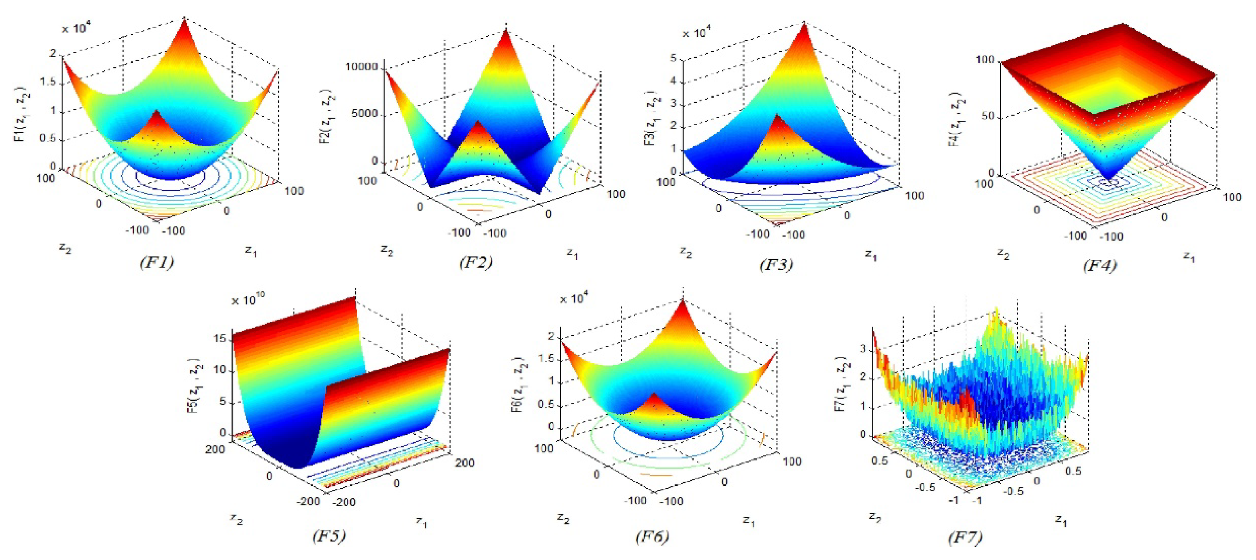
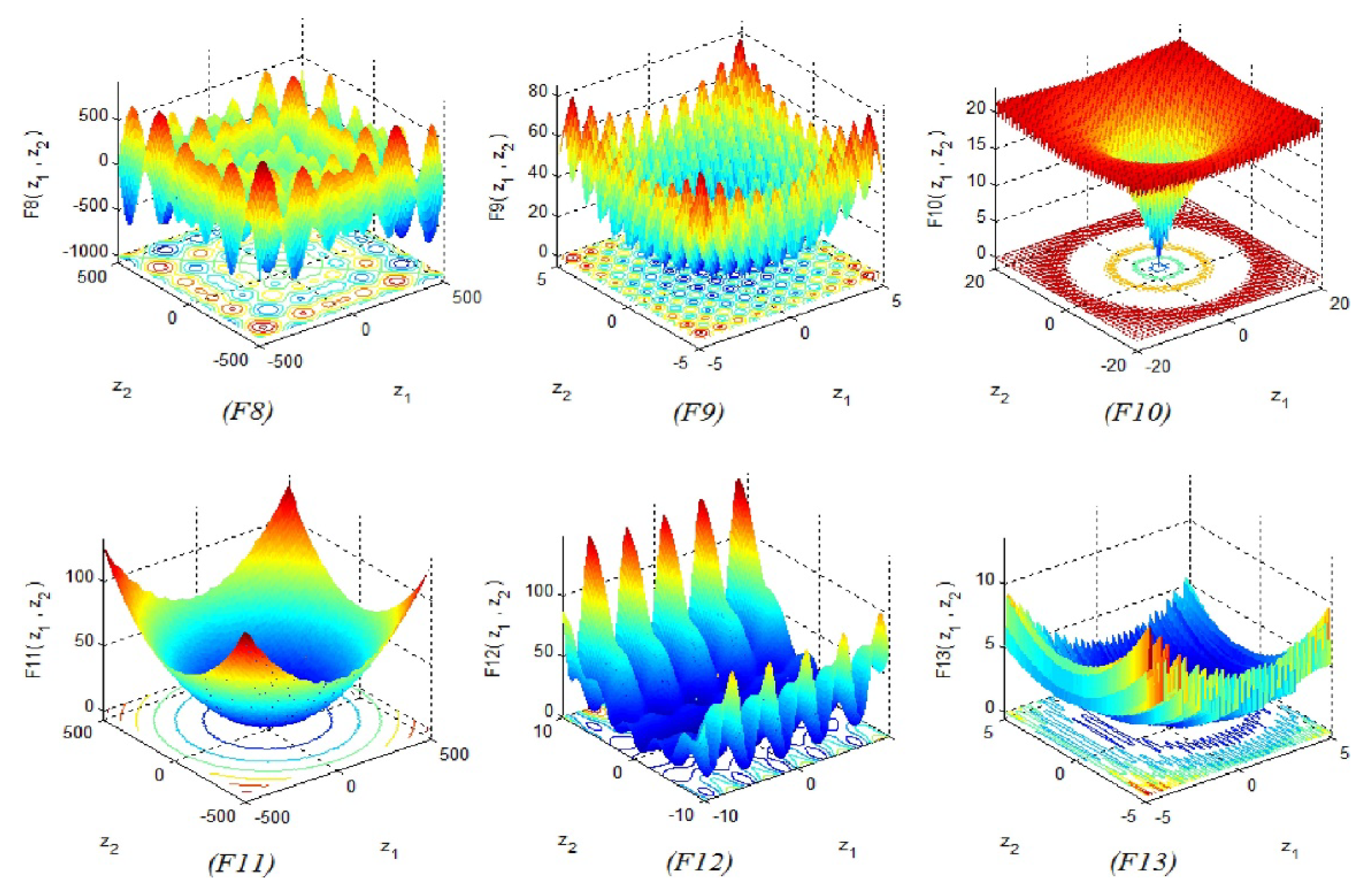
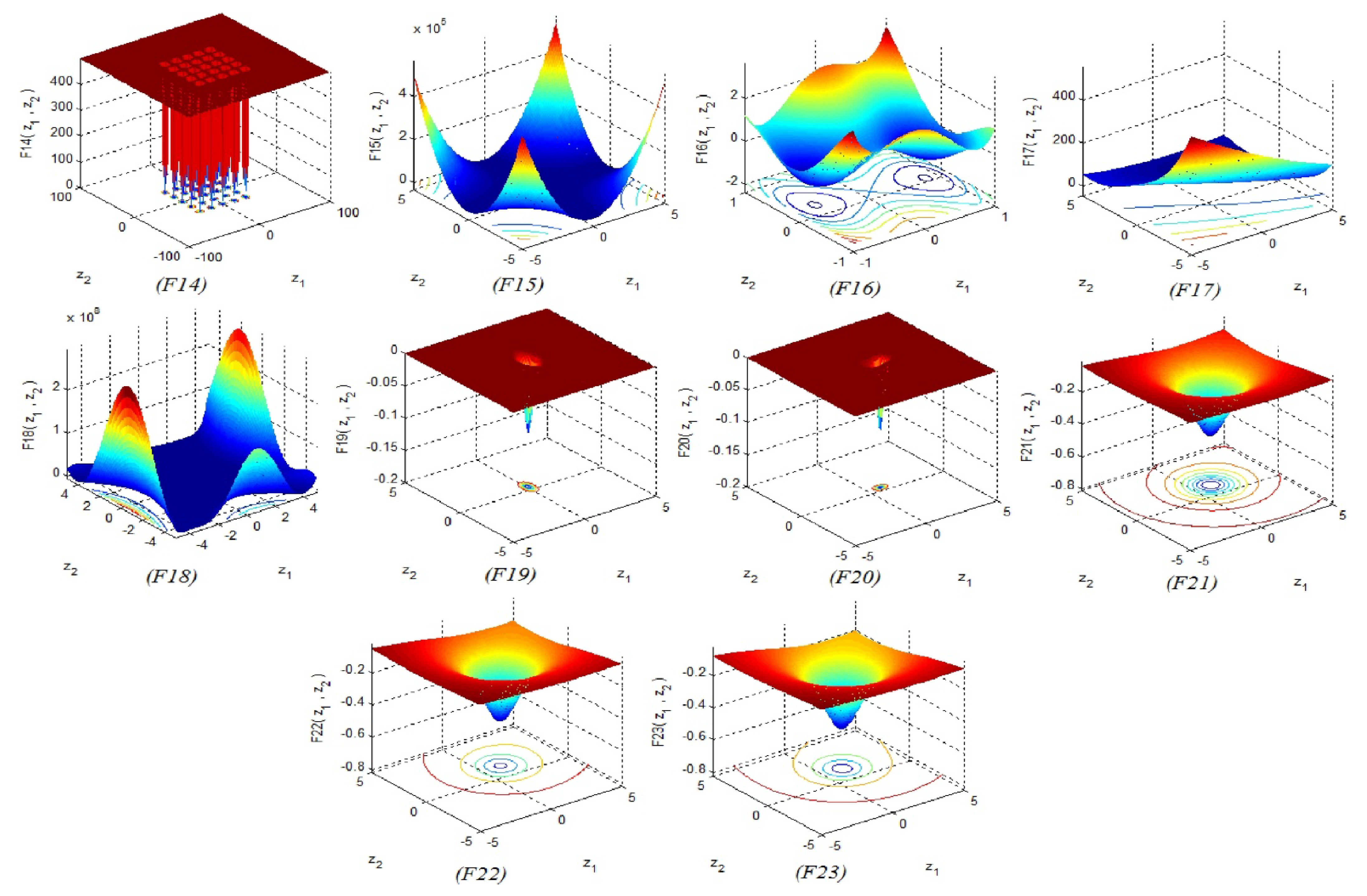
In the first category of the benchmark test functions, the unimodal benchmark functions (F₁–F₇), there is only one global optimum, and there are no local optima. Thus, that makes it suitable for the analysis of the algorithm’s convergence speed and exploitation capability. The second category consists of 9 benchmark functions (F₈–F₁₃), and 10 benchmark functions (F₁₄–F₂₃) are included in the third category. The second and third categories of the benchmark test functions are useful for examining the algorithm’s local optima avoidance and exploration capability as these functions consist of many local optima in addition to the global optimum. The 3D plot of all the benchmark functions is illustrated in Figure 3, Figure 4 and Figure 5 [3].

4. REA for Quadrotor Control Application

After we have tested our algorithm on the benchmark test functions, the proposed algorithm is implemented for the quadrotor control application. The goal here is to tune the controller’s parameters with the proposed algorithm to search for the best performance optimal parameter.

4.1. Mathematical Model of The Quadrotor

Before we can implement the algorithm, it is necessary to define the quadrotor’s dynamic equation first. The dynamics equation of the quadrotor used here is based on the Newton-Euler theory. Several assumptions must be considered to derive these equations, which are [43] (1) the structure of the quadrotor is rigid and symmetrical, (2) the center of gravity of the quadrotor and the origin of the body-fixed frame must coincide, and (3) thrust and drag forces are proportional to the square of the rotor’s speed. The complete dynamics equation of the quadrotor is given in Equation (5) below [44]:

$$\begin{gathered} \ddot{\varphi }=\frac{\left(I_y-I_z\right)}{I_x}\dot{\psi }\dot{\theta }+\frac{l}{I_x}{U}_2 \\ \ddot{\theta }=\frac{\left(I_z-I_x\right)}{I_y}\dot{\psi }\dot{\varphi }+\frac{l}{I_y}{U}_3 \\ \ddot{\psi }=\frac{\left(I_x-I_y\right)}{I_z}\dot{\theta }\dot{\varphi }+\frac{1}{I_z}{U}_4 \\ \ddot{x}=\left(\cos \varphi \sin \theta \cos \psi +\sin \varphi \sin \psi \right)\frac{1}{m}{U}_1 \\ \ddot{y}=\left(\cos \varphi \sin \theta \sin \psi -\sin \varphi \cos \psi \right)\frac{1}{m}{U}_1 \\ \ddot{z}=-g+\left(\cos \varphi \cos \theta \right)\frac{1}{m}{U}_1 \end{gathered}$$

(5)

where I_x, I_y, I_z are the inertia in the x, y, and z-axis, respectively, l is the length of the rotor to the center of the quadrotor, m is the mass of the quadrotor, g is the gravity constant, and U_i(I = 1, 2, 3, 4) is the control input to the quadrotor. It can be expressed as in Equation (6) below. The parameters of the quadrotor used are given in

Table 1. Parameters of the quadrotor.

Parameter	Value	Unit
Mass, m	1.12	Kg
Arm length, l	0.23	m
Inertia x-axis, Ix	1.19 × 10−2	Kgm2
Inertia y-axis, Iy	1.19 × 10−2	Kgm2
Inertia z-axis, Iz	2.23 × 10−2	Kgm2
Rotor inertia, Jr	8.50 × 10−4	Kgm2
Thrust coefficient, b	7.73 × 10−6	Ns2
Drag coefficient, d	1.28 × 10−7	Nms2

below [45]:

$$\begin{gathered} U_1=b\left({\mathsf{\Omega }}_1^2+{\mathsf{\Omega }}_2^2+{\mathsf{\Omega }}_3^2+{\mathsf{\Omega }}_4^2\right) \\ {U}_2=b\left(-{\mathsf{\Omega }}_2^2+{\mathsf{\Omega }}_4^2\right) \\ {U}_3=b\left(-{\mathsf{\Omega }}_1^2+{\mathsf{\Omega }}_3^2\right) \\ {U}_4=d\left(-{\mathsf{\Omega }}_1^2+{\mathsf{\Omega }}_2^2-{\mathsf{\Omega }}_3^2+{\mathsf{\Omega }}_4^2\right) \end{gathered}$$

(6)

4.2. A Hybrid PD2-LQR Controller

In this study, only four states will be chosen for the control purpose: the altitude (z) and the three Euler angles (ϕ, θ, ψ). In order to control and stabilize the system, an appropriate control law for the system must be designed to accomplish the desired control performance. The structure of the hybrid PD2-LQR controller is depicted in Figure 6 below:

Let a state-space representation of a linear system is described as in Equation (7) below:

$$\dot{X}=AX+BU$$

(7)

Now, from the above control structure, the control law of the system can be represented as in Equation (8) below:

$$U=-K_T+E{K}_e$$

(8)

From there, we can see that the gain K_T is the total gain of the original LQR controller’s gain and the PD2 controller’s gain and is defined as Equation (9) below, and Ke is the system’s error gain.

$$K_T=KX+K_{p}CX+\left(K_{d1}+K_{d2}\right)C\frac{dX}{dt}$$

(9)

E is the error signal between the output y and the reference input defined in Equation (10). Now, combining the Equations (9) and (10), the control input of the system can be expressed as Equation (11) below:

$$E=-y+r_d=-CX+r_d$$

(10)

$$U=-KX-K_{p}CX-K_{e}CX-\left(K_{d1}+K_{d2}\right)C\frac{dX}{dt}+K_e{r}_d$$

(11)

4.3. Objective Function

The evaluation of the control performance will be determined based on the objective function. Generally, the typical objective functions that are mostly used to optimize the controller’s parameter are Integral Absolute Error (IAE), Integral Square Error (ISE), Integral Time Absolute Error (ITAE), and Integral Time Square Error (ITSE). The IAE objective function was used in this study to optimize the controller’s parameters so that the error between input/output of the system is minimum/0.

Hence, the algorithm considers the system’s overshoot (which is also related to the rise time) and steady-state error to achieve this. With these interdependent relationships among parameters, we can be sure that the algorithm minimizes all involved parameters (or at least within the acceptable limit), so the input/output of the system is minimal.

Additionally, the objective function has been modified to accommodate some other performance indexes such as the rise time (RT), percentage overshoot (OS), and steady-state error (SSE). This modification was made based on the findings made by [44], who claimed that the system’s response shows an improvement where a faster rise time, short settling time, small overshoot, and minimal steady-state error are produced when such objective function is used. The IAE and the new objective function are given in the Equations (12) and (13) respectively:

$$IAE={{\displaystyle \int }}_0^T\left|e\left(t\right)\right|dt$$

(12)

$$IAE={{\displaystyle \int }}_0^T\left|e\left(t\right)\right|dt$$

(13)

4.4. Experimental Setup

The parameter settings for the proposed algorithm and other selected algorithms are shown in

Table 2. Parameter setting for the algorithm.

No.	Algorithms	Parameters	Value
1	Random Explosion Algorithm (REA)	No. of fragments, nF Explosion radius, re c	90 (triple of the population size) (Ub, ~0) 70
2	Particle Swarm Optimization (PSO)	Inertia coefficient, w Cognitive and social coefficient, c1, c2	0.75 1.8, 2
3	Artificial Bee Colony (ABC)	Parameter limit	Number of food source × dimension, (number of food source = number of populations, dimension = dimension of solution)
4	Genetic Algorithm (GA)	Crossover Mutation	0.9 0.05
5	Differential Evolution (DE)	Crossover Scale factor	0.9 0.5
6	Multi-Verse Optimizer (MVO)	Wormhole existence probability Traveling distance rate	(0.2, 1) (0.6, 1)
7	Moth Flame Optimizer (MFO)	Convergence constant Logarithmic spiral	(−1, −2) 0.75
8	Firefly Algorithm (FA)	Randomness factor, α Light absorption coefficient, γ	0.2 1
9	Sooty Tern Optimization Algorithm (STOA)	Controlling variable, Cf Sa	2 (Cf, 0)

. These parameters are set according to the literature reported. For our algorithm, the selection of the parameter is made based on several preliminary experiments. We found that our algorithm works quite well with the parameters setting reported in Table 2. However, it is worth noting some guidelines for tuning these parameters.

Firstly, for the number of fragments, it is advisable to choose based on the number of populations, the complexity of the problem, and how big the search space is. Suppose the number of populations is less than 10. In that case, it is recommended to use a high value of the number of fragments such as five or more times of population size, while for populations greater than 10, it is sufficient to use only triple times of population size (used in this study).

For a complicated problem, it is recommended to increase the number of fragments instead of the number of the population since it only has a minor effect on the computational time, while increasing the population size will increase the computational time significantly. For a small search space, it is sufficient to use a low number of fragments (triple of populations size), but for a large search space, it is recommended to use a high number of fragments because the search radius will be larger, so low number of fragments is not appropriate to search such large space.

Secondly, for the parameter constant, c, it is advisable to choose based on the maximum number of iterations. In this study, with a maximum iteration of 1000, we use c = 70, but the range can be between 70–100 where the algorithm can still perform sufficiently. Different maximum iteration has a different range of c value. This value must be chosen carefully since it affects the search radius that will indirectly affect the algorithm’s exploration and exploitation capability.

Experimentation and algorithms are implemented in the MATLAB R2020a version (MathWorks, Natick, MA, USA), and the simulation was run on the Microsoft Windows 10 with 64-bit on Core i5 processor with 2.4 GHz and 8 GB of memory. The mean and standard deviation of the best fitness achieved until the last iteration is calculated as the performance metrics. For each of the benchmark test functions, the algorithms were run for 10 separate runs, with each run using 1000 times of iterations.

5. Results and Discussion

The simulation and experimentation to evaluate the performance of the proposed algorithm are presented in this section. The algorithm was tested on 23 benchmark test functions. The performance of the proposed algorithm is also validated by comparing it with eight other well-known algorithms. Particle Swarm Optimization (PSO) [21], Artificial Bee Colony (ABC) [23], Genetic Algorithm (GA) [4], Differential Evolution (DE) [5], Multi-Verse Optimizer (MVO) [46], Moth Flame Optimizer (MFO) [47], Firefly Algorithm (FA) [28], and Sooty Tern Optimization Algorithm (STOA) [48] are the algorithms chosen.

For all algorithms, the number of search agents (population) used is 30, the maximum iteration is set to be 1000, and each algorithm was run for 10 separate runs. Furthermore, the controller’s performance using the proposed algorithm is also evaluated similarly to the first part of this study by comparing the result with the different algorithms used. The controller’s performance will be assessed in terms of the rise time, settling time, percentage overshoot, steady-state error, and RMSE of a system’s response.

5.1. Performance Comparison of REA

A comparative study with eight other well-known algorithms on unimodal, multimodal, and fixed dimensional multimodal benchmark test functions was conducted to demonstrate the proposed algorithm’s performance. The unimodal benchmark functions consist of one global optimum and are therefore suitable for analyzing the algorithm’s exploitation capability. According to the results in

Table A4. Minimization results for the Unimodal, Multimodal, and Fixed-dimension Multimodal benchmark functions. Results were averaged from 10 individual runs, with a population size of N = 30 and the maximum number of iterations of T = 1000.

	F	REA		PSO		ABC		GA		DE		MVO		MFO		FA		STOA
		Ave	Std	Ave	Std	Ave	Std	Ave	Std	Ave	Std	Ave	Std	Ave	Std	Ave	Std	Ave	Std
Unimodal	F1	9.72E-58	2.40E-58	1.82E-08	2.62E-08	8.79E-17	2.14E-17	6.76E-02	1.36E-01	1.13E-43	3.57E-43	4.08E-03	1.48E-03	2.52E-29	6.14E-29	7.58E-18	2.63E-18	6.58E-38	1.28E-37
	F2	7.91E-30	9.88E-31	6.42E-06	6.62E-06	3.12E-16	6.94E-17	3.71E-03	6.53E-03	2.01E-28	4.21E-28	1.69E-02	4.40E-03	1.32E-18	1.91E-18	6.80E-10	8.94E-11	5.21E-22	5.92E-22
	F3	1.08E-57	1.81E-58	2.22E-02	2.21E-02	1.97E+01	1.64E+01	2.23E+02	1.19E+02	1.85E-04	3.46E-04	2.79E-02	1.93E-02	1.37E-06	2.29E-06	1.24E-17	3.71E-18	1.20E-23	2.88E-23
	F4	1.81E-29	1.56E-30	2.00E-02	1.82E-02	5.97E-03	2.09E-03	1.19E+00	3.94E-01	1.47E+00	1.47E+00	4.66E-02	1.92E-02	2.53E-01	5.14E-01	1.62E-09	2.55E-10	2.45E-14	3.67E-14
	F5	4.81E+00	1.71E+00	5.68E+00	1.62E+00	1.24E-01	1.51E-01	3.03E+01	2.80E+01	4.73E+00	2.44E+00	6.40E+01	9.78E+01	2.89E+01	5.21E+01	5.93E-01	1.51E+00	7.19E+00	4.23E-01
	F6	0.00E+00	0.00E+00	6.83E-08	1.22E-07	9.84E-17	5.24E-17	2.20E-02	2.34E-02	9.27E-20	2.93E-19	3.97E-03	2.37E-03	9.49E-31	1.38E-30	8.23E-18	2.58E-18	1.25E-01	1.76E-01
	F7	1.34E-04	6.06E-05	1.36E-03	6.20E-04	9.02E-03	4.40E-03	4.28E-03	5.70E-03	1.81E-03	6.87E-04	2.13E-03	1.13E-03	6.52E-03	4.18E-03	1.90E-04	2.23E-04	7.70E-04	6.85E-04
Multimodal	F8	−3.10E+02	3.85E+02	−2.78E+02	3.24E+02	−4.19E+02	9.59E-13	−3.67E+02	9.99E+01	−3.80E+02	1.55E+02	−3.00E+02	2.62E+02	−3.30E+02	3.53E+02	−3.55E+02	2.77E+02	−2.64E+02	2.48E+02
	F9	1.60E+01	6.25E+00	6.88+E00	2.46E+00	0.00E+00	0.00E+00	2.31E-03	4.13E-03	3.29E+00	3.81E+00	1.56E+01	6.29E+00	1.91E+01	8.15E+00	8.16E+00	3.03E+00	6.97E-01	2.20E+00
	F10	4.44E-15	0.00E+00	4.43E-05	3.12E-05	7.64E-15	2.02E-15	3.87E-02	5.68E-02	7.13E-11	2.25E-10	2.51E-02	5.34E-03	5.51E-15	1.72E-15	1.10E-09	1.84E-10	3.98E+00	8.40E+00
	F11	2.62E-01	1.48E-01	1.69E-01	9.87E-02	1.72E-03	5.45E-03	6.11E-02	3.76E-02	3.72E-02	2.01E-02	3.61E-01	1.23E-01	2.13E-01	1.55E-01	6.08E-02	1.32E-02	2.25E-02	5.29E-02
	F12	4.71E-32	1.15E-47	3.77E-10	4.12E-10	7.88E-17	2.13E-17	2.43E-04	2.01E-04	4.76E-32	1.23E-33	1.36E-04	7.16E-05	9.33E-02	2.10E-01	7.03E-20	1.97E-20	2.81E-02	1.50E-02
	F13	1.35E-32	2.89E-48	3.49E-09	7.31E-09	9.41E-17	1.39E-17	4.71E-03	5.50E-03	1.40E-32	1.56E-33	1.82E-03	3.55E-03	4.39E-03	5.67E-03	3.99E-19	5.62E-20	1.33E-01	7.34E-02
Fixed-dimension Multimodal	F14	9.98E-01	0.00E+00	4.06E+00	2.52E+00	9.98E-01	1.05E-16	9.98E-01	1.44E-10	9.98E-01	0.00E+00	9.98E-01	4.70E-12	1.79E+00	1.30E+00	9.98E-01	2.67E-16	1.59E+00	9.58E-01
	F15	3.07E-04	5.71E-20	4.32E-03	8.46E-03	6.37E-04	9.97E-05	1.40E-03	5.48E-04	5.88E-04	4.32E-04	6.70E-03	9.43E-03	3.02E-03	6.10E-03	3.07E-04	1.86E-09	1.05E-03	3.74E-04
	F16	−1.03E+00	0.00E+00	−1.03E+00	0.00E+00	−1.03E+00	1.96E-16	−1.03E+00	2.52E-06	−1.03E+00	0.00E+00	−1.03E+00	1.10E-07	−1.03E+00	0.00E+00	−1.03E+00	1.66E-16	−1.03E+00	4.31E-07
	F17	3.98E-01	0.00E+00	3.98E-01	0.00E+00	3.98E-01	0.00E+00	3.98E-01	3.54E-07	3.98E-01	0.00E+00	3.98E-01	2.10E-07	3.98E-01	0.00E+00	3.98E-01	0.00E+00	3.98E-01	2.04E-05
	F18	3.00E+00	4.68E-16	3.00E+00	2.09E-16	3.00E+00	4.53E-06	3.00E+00	2.47E-07	3.00E+00	1.48E-15	3.00E+00	9.97E-07	3.00E+00	1.55E-15	3.00E+00	7.40E-16	3.00E+00	7.04E-06
	F19	−3.86E+00	4.68E-16	−3.86E+00	8.24E-16	−3.86E+00	5.34E-16	−3.86E+00	1.01E-04	−3.86E+00	9.36E-16	−3.86E+00	2.85E-07	−3.86E+00	9.36E-16	−3.86E+00	4.91E-16	−3.85E+00	2.31E-05
	F20	−3.20E+00	9.26E-08	−3.29E+00	5.74E-02	−3.32E+00	3.63E-16	−3.07E+00	6.70E-01	−3.26E+00	6.27E-02	−3.25E+00	6.17E-02	−3.23E+00	6.52E-02	−3.27E+00	6.14E-02	−3.01E+00	1.43E-01
	F21	−1.02E+01	1.87E-15	−6.90E+00	3.54E+00	−1.02E+01	1.87E-15	−7.17E+00	3.86E+00	−1.02E+01	5.92E-16	−7.62E+00	2.67E+00	−7.39E+00	3.01E+00	−1.02E+01	2.37E-15	−5.50E+00	4.31E+00
	F22	−1.04E+01	0.00E+00	−7.67E+00	3.58E+00	−1.04E+01	5.13E-12	−8.11E+00	3.70E+00	−1.04E+01	2.37E-15	−7.81E+00	3.43E+00	−8.21E+00	3.54E+00	−1.04E+01	1.57E-15	−6.45E+00	5.05E+00
	F23	−1.05E+01	0.00E+00	−6.71E+00	4.05E+00	−1.05E+01	3.19E-15	−1.00E+01	1.70E+00	−1.05E+01	1.87E-15	−9.46E+00	2.27E+00	−8.47E+00	3.39E+00	−1.05E+01	1.32E-15	−7.25E+00	4.38E+00

Note: The green value indicates the algorithm’s best minimum value, while the red value indicates the worst value obtained by the algorithm.

in Appendix B, REA provided a competitive outcome compared to the others.

In particular, REA outperforms the other algorithms on F₁, F₂, F₃, F₄, F₆, and F₇ benchmark functions with the lowest mean and standard deviation. For F₅ only, with the lowest mean and standard deviation, ABC performs better than REA. Based on these results, we can say that REA can provide superior performance in exploiting the optimum with a faster convergence speed than the other algorithms.

Unlike the unimodal benchmark functions, the multimodal benchmark functions consist of many local optima, which increase exponentially with the dimension. For this reason, it makes them suitable for evaluating the algorithm’s exploration capability and local stagnation avoidance. Based on the findings reported in Table A4 in Appendix B for multimodal benchmark functions (F₈–F₁₃) and fixed dimension multimodal benchmark functions (F₁₄–F₂₃), we can see that REA has a good exploration capability in finding the global optimum solution for the benchmark functions tested. These results show that out of the 16 (F₈–F₂₃) benchmark functions tested, REA can give a better performance for 12 benchmark functions (F₁₀, F₁₂, F₁₃, F₁₄, F₁₅, F₁₆, F₁₇, F₁₈, F₁₉, F₂₁, F₂₂, and F₂₃) while ABC is outperforming REA for F₈, F₉, F₁₁, and F₂₀ benchmark functions.

However, it can also be noted that some other algorithms produce the same outcome as REA for fixed dimension multimodal benchmark functions. In F₁₄, the algorithms that can give the same average value as REA are ABC, GA, DE, MVO, and FA, but only DE has the same standard deviation as REA. In F₁₅, only FA has the same average value as REA. In F₁₆, PSO, DE, and MFO have the same average value and standard deviation as REA, while the rest of the algorithms only have the same average value. In F₁₇, PSO, ABC, DE, MFO, and FA have the same average value and standard deviation as REA, while the rest only have the same average value.

In F₁₈, all algorithms produced the same results for the average value, but only PSO has the best standard deviation. In F₁₉, all algorithms except STOA have the same average value as REA, while only REA has the best standard deviation. In F₂₁, REA, ABC, DE, and FA have the same average value, but only DE has the best standard deviation. In F₂₂ and F₂₃, REA, ABC, DE, and FA have the same average value, but only REA has the best standard deviation. These findings show that REA can obtain a very competitive outcome in most multimodal benchmark functions and has good merit in exploration capability and local optima avoidance.

5.2. Convergence Analysis

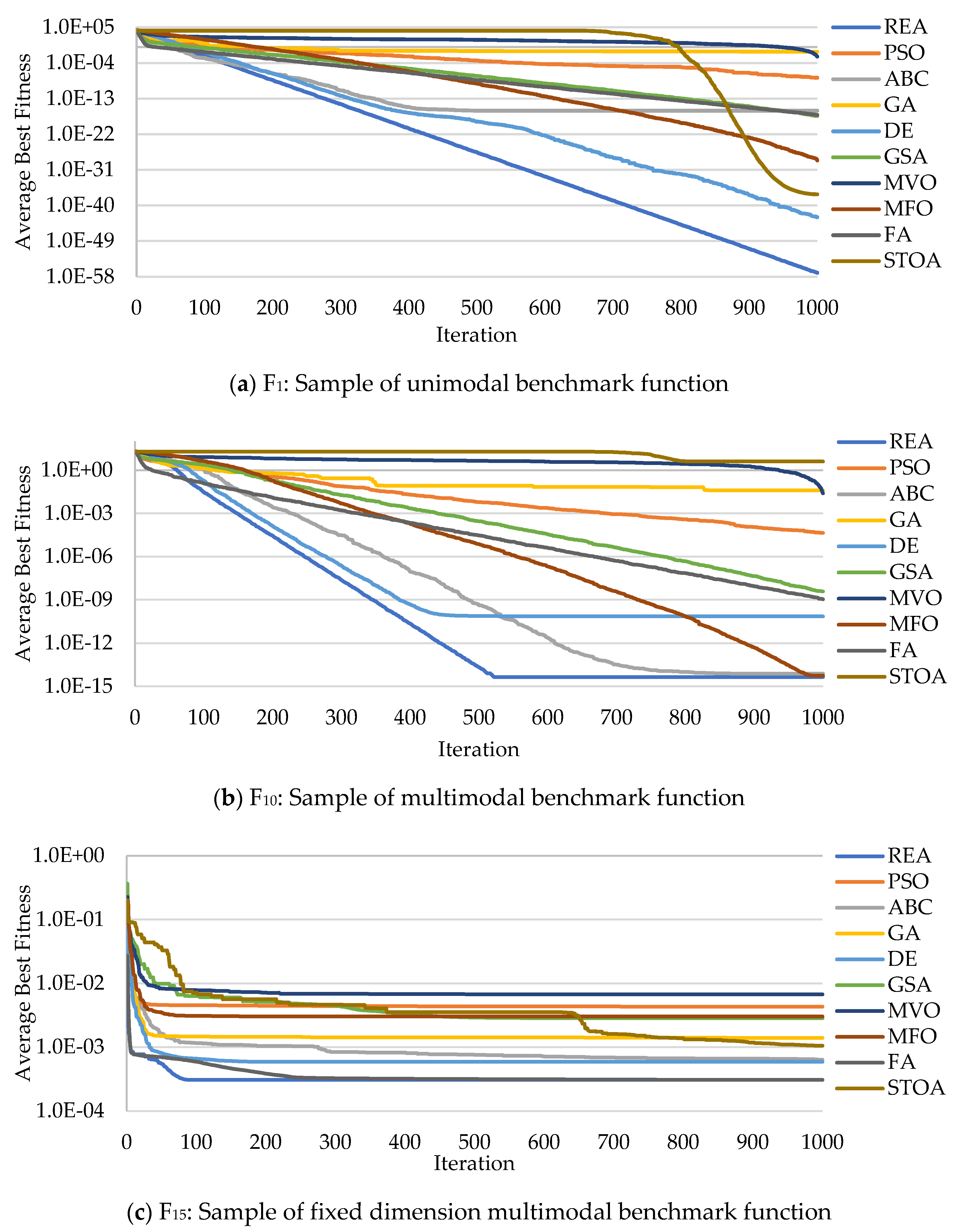
The convergence curve of all algorithms is plotted in Figure 7 to visualize the REA algorithm’s evolution over iterations. For this analysis, three distinct benchmark functions were contemplated: F₁ (for unimodal benchmark functions), F₁₀ (for multimodal benchmark functions), and F₁₅ (for fixed dimension multimodal benchmark function). These figures are plotted to illustrate the speed at which the algorithms converge and the algorithm’s exploration and exploitation capability. From these figures, we can see that REA has a very competitive result compared to the other algorithms.

At the initial stage of the iteration process, we can see that REA can explore the promising region in the search space and quickly converge towards a global optimum compared to other algorithms. After a certain amount of iteration, the REA finally converges towards the optimum when the final iteration is reached. With these findings, we can conclude that REA has a better balance between exploration and exploitation capability to find a global optimum. REA’s convergence speed is also faster and more accurate than the other algorithms.

5.3. Performance Comparison of REA Based PD2-LQR Controller

Since the number of populations affects the algorithms’ performance, all algorithm’s population size was chosen to be the same. The specific parameters that describe the properties of the algorithm were selected according to the literature stated before. The system’s initial condition is set to be (0, 0, 0, 0), and the final state will be (1, 1, 1, 1) for the roll, pitch, yaw, and altitude motions, respectively.

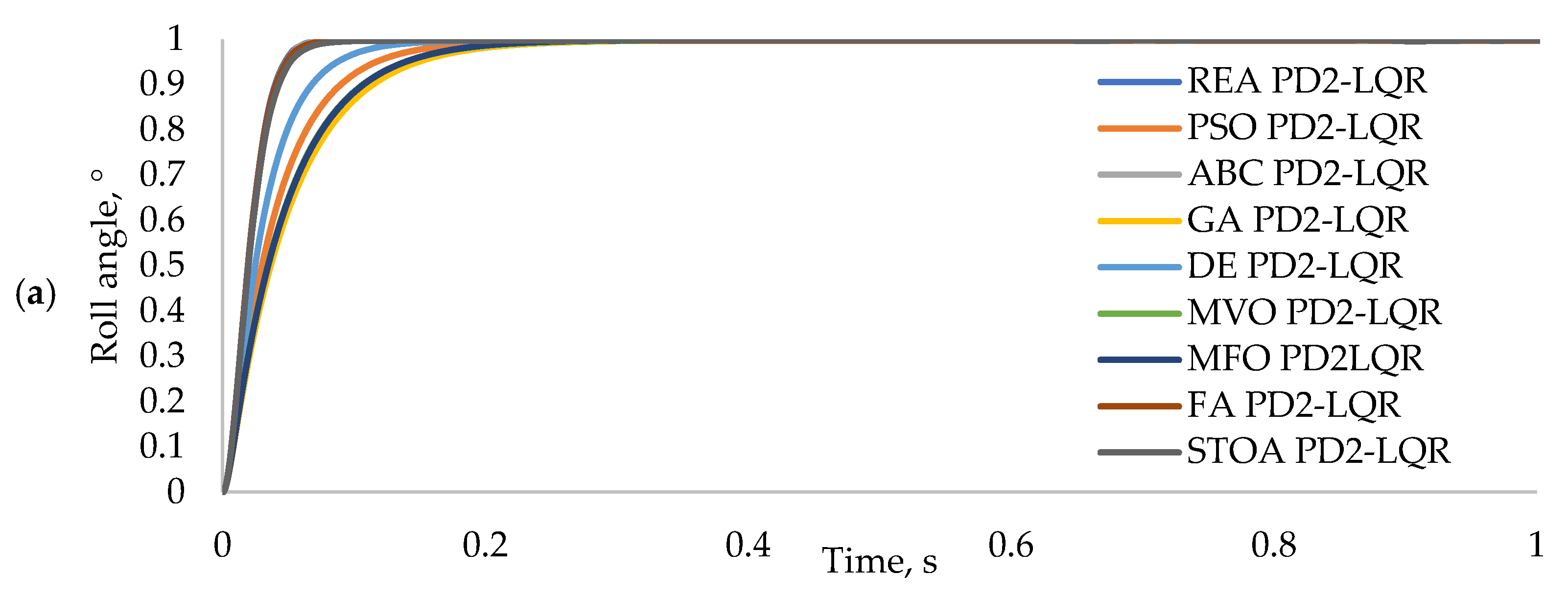
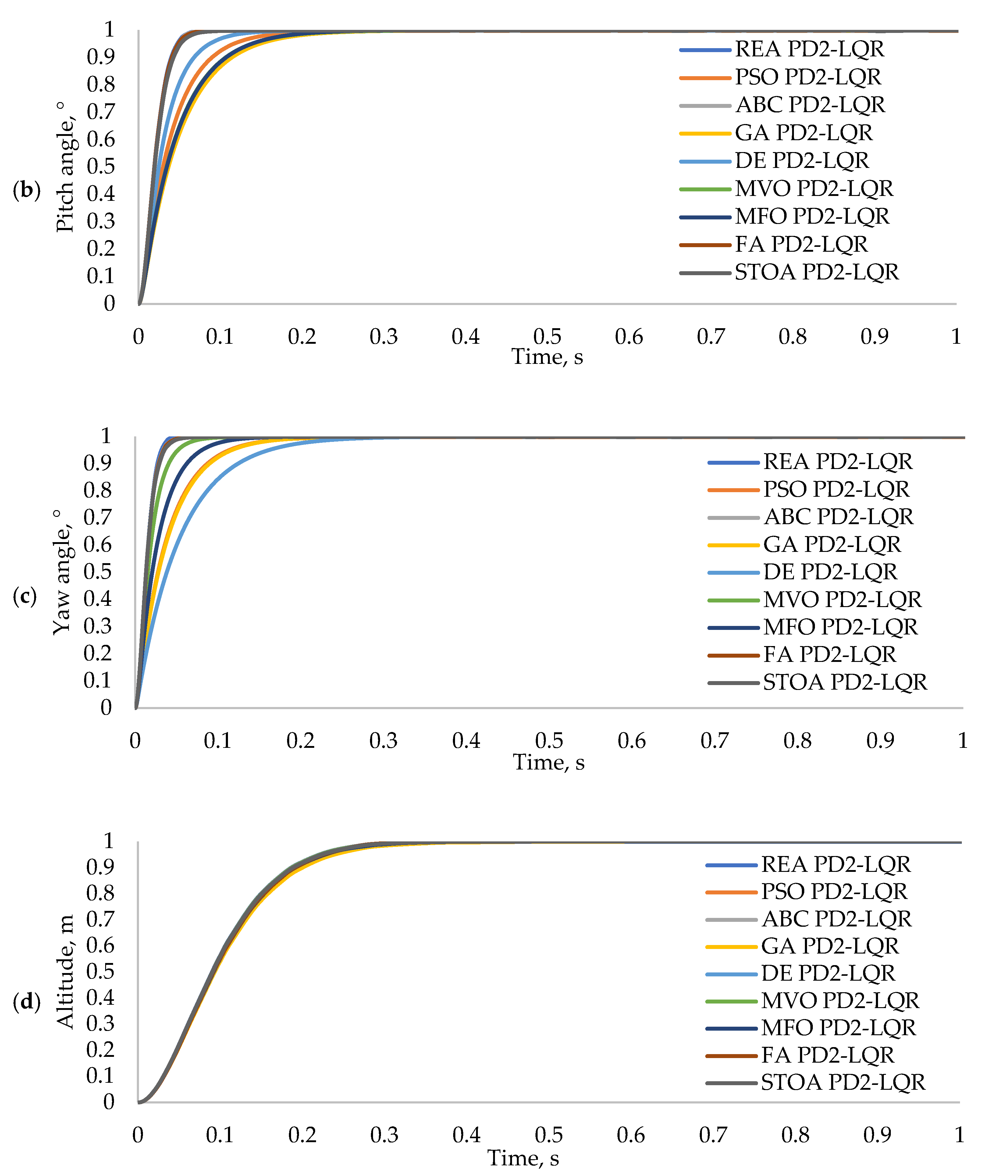
For evaluation purposes, there are five performance criteria used for the comparisons: rise time, settling time, percentage overshoot, steady-state error, and RMSE of the system’s response. The system’s response using the REA PD2-LQR controller in comparison with various other algorithms is presented in Figure 8 for the roll, pitch, yaw, and altitude motions. It could be evident that from the simulation result obtained in

Table 3. Performance comparison of the controller for all motion.

Motion	Algorithm	Rise Time, s	Settling Time, s	Overshoot, %	Steady-State error	RMSE
Roll	REA	0.03361	0.05713	0.00000E+00	6.44466E-06	0.23449
	PSO	0.08200	0.15520	0.00000E+00	3.20000E-03	0.22620
	ABC	0.03441	0.05765	0.00000E+00	5.65577E-04	0.24068
	GA	0.10570	0.19360	0.00000E+00	7.61930E-04	0.21840
	DE	0.06060	0.11330	0.00000E+00	7.05810E-04	0.22930
	MVO	0.09870	0.18210	0.00000E+00	1.50000E-03	0.21630
	MFO	0.09909	0.18101	2.32631E-02	1.73851E-04	0.21664
	FA	0.03422	0.05853	0.00000E+00	8.42488E-04	0.23436
	STOA	0.03677	0.06488	0.00000E+00	2.30451E-03	0.23422
Pitch	REA	0.03361	0.05713	0.00000E+00	6.44466E-06	0.23449
	PSO	0.08200	0.15520	0.00000E+00	3.20000E-03	0.22620
	ABC	0.03441	0.05765	0.00000E+00	5.65577E-04	0.24068
	GA	0.10570	0.19360	0.00000E+00	7.61930E-04	0.21840
	DE	0.06060	0.11330	0.00000E+00	7.05810E-04	0.22930
	MVO	0.09870	0.18210	0.00000E+00	1.50000E-03	0.21630
	MFO	0.09909	0.18101	2.32631E-02	1.73851E-04	0.21664
	FA	0.03422	0.05853	0.00000E+00	8.42488E-04	0.23436
	STOA	0.03677	0.06488	0.00000E+00	2.30451E-03	0.23422
Yaw	REA	0.02294	0.03742	0.00000E+00	1.17230E-04	0.20431
	PSO	0.08120	0.15000	0.00000E+00	2.40000E-03	0.18440
	ABC	0.02400	0.04160	0.00000E+00	6.79900E-04	0.20090
	GA	0.08390	0.15290	0.00000E+00	9.52840E-04	0.17360
	DE	0.11720	0.21080	4.50000E-03	1.34400E-04	0.16930
	MVO	0.03580	0.06770	0.00000E+00	1.60000E-03	0.19580
	MFO	0.05722	0.10487	1.55229E-02	9.20977E-05	0.18574
	FA	0.02437	0.04236	0.00000E+00	9.06897E-04	0.20156
	STOA	0.02537	0.04526	0.00000E+00	7.96213E-04	0.19670
Altitude	REA	0.15748	0.26129	0.00000E+00	3.93389E-06	0.40235
	PSO	0.16270	0.27240	1.71030E-05	8.18330E-10	0.39760
	ABC	0.15810	0.26280	0.00000E+00	1.81070E-04	0.40250
	GA	0.16879	0.28837	0.00000E+00	1.14450E-05	0.40447
	DE	0.16090	0.27070	0.00000E+00	1.92650E-04	0.40040
	MVO	0.15850	0.26310	2.94720E-06	6.36660E-11	0.39700
	MFO	0.16196	0.27312	0.00000E+00	7.35813E-05	0.40057
	FA	0.16110	0.26372	2.64186E-05	1.92583E-11	0.40152
	STOA	0.15958	0.26455	1.52380E-04	3.30136E-09	0.40270

Note: The green value indicates good performance, while the red value indicates bad performance.

and the step response depicted in Figure 8 below, all of the controllers were able to drive the quadrotor to the desired reference altitude and angle and manage to stabilize the system in a very fast period with a good performance.

However, there is still a significant difference in the performance response among these controllers. From these figures and table, we can see that the REA based controller produced the best overall performance in all motion. In contrast, the worst overall performance can be said to be GA based controller in roll, pitch, and altitude motion and DE based controller in yaw motion.

Nevertheless, to properly visualize how much the proposed REA based controller can improve the system’s performance, we need to calculate and show the percentage improvement for better understanding. The REA based controller’s percentage improvement with respect to the other individual controllers is presented in

Table 4. Percentage improvement of the REA based controller for all motions.

Motion	Algorithm	Rise Time	Settling Time	Overshoot	Steady-State Error	RMSE
Roll	PSO	−59.01713	−63.19033	-	−99.79860	3.66322
	ABC	−2.34674	−0.90504	-	−98.86052	−2.57302
	GA	−68.20629	−70.49142	-	−99.15417	7.36547
	DE	−44.54463	−49.57757	-	−99.08691	2.26175
	MVO	−65.95142	−68.62789	-	−99.57036	8.40786
	MFO	−66.08584	−68.43815	−100.00000	−96.29299	8.23617
	FA	−1.79735	−2.39915	-	−99.23504	0.05346
	STOA	−8.60110	−11.94595	-	−99.72035	0.11473
Pitch	PSO	−59.01713	−63.19033	-	−99.79860	3.66322
	ABC	−2.34674	−0.90504	-	−98.86052	−2.57302
	GA	−68.20629	−70.49142	-	−99.15417	7.36547
	DE	−44.54463	−49.57757	-	−99.08691	2.26175
	MVO	−65.95142	−68.62789	-	−99.57036	8.40786
	MFO	−66.08584	−68.43815	−100.00000	−96.29299	8.23617
	FA	−1.79735	−2.39915	-	−99.23504	0.05346
	STOA	−8.60110	−11.94595	-	−99.72035	0.11473
Yaw	PSO	−71.75218	−75.05260	-	−95.11540	10.79617
	ABC	−4.42820	−10.04543	-	−82.75771	1.69643
	GA	−72.66123	−75.52577	-	−87.69674	17.68902
	DE	−80.42898	−82.24805	−100.00000	−12.77503	20.67817
	MVO	−35.92952	−44.72511	-	−92.67310	4.34532
	MFO	−59.91605	−64.31817	−100.00000	27.28919	9.99415
	FA	−5.87671	−11.66429	-	−87.07347	1.36461
	STOA	−9.58509	−17.32273	-	−85.27651	3.86803
Altitude	PSO	−3.21109	−4.07913	−100.00000	480,621.16279	1.19500
	ABC	−0.39497	−0.57517	-	−97.82742	−0.03694
	GA	−6.70340	−9.39138	-	−65.62806	−0.52366
	DE	−2.12831	−3.47675	-	−97.95801	0.48734
	MVO	−0.64634	−0.68854	−100.00000	6,178,842.43626	1.34794
	MFO	−2.77157	−4.33162	-	−94.65369	0.44420
	FA	−2.25051	−0.92294	−100.00000	20,426,901.9929	0.20802
	STOA	−1.31845	−1.23301	−100.00000	119,059.40416	−0.08551

Note: The green value indicates the performance was improved, while the red value indicates the performance was not improved.

for the roll, pitch, yaw, and altitude motion.

From the table above, we can see that the improvement is very significant and very good in terms of the rise time and settling time for all four motions. The REA based controller seems to outperform all the other controllers. The overshoot and steady-state error of a certain controller is minimal, and thus we can neglect these values or approximate them to zero.

Finally, the value of RMSE for the REA based controller is not likely to have much improvement, but if we look carefully, it only has a small difference; thus, it still can be acceptable. For example, let us take the DE based controller for yaw motion with the highest percentage increase; we can see that it is only 0.03501 indifferent with the REA based controller. Therefore, we can conclude that the REA based controller can produce a better overall result than the other controllers.

5.4. Robustness Test of REA Based PD2-LQR Controller

In this section, the REA-based controller’s robustness test under the presence of unknown external disturbance and sensor noise will be presented. This simulation was conducted to simulate the real-world application of the quadrotor. When flying in an outdoor environment, the quadrotor is constantly subjected to unknown disturbance such as wind gust [49]. It is also known that when implemented on a real quadrotor system, the feedback data from the sensor are always noisy and distorted due to the mechanical vibration produced by the electronic equipment [50]. Usually, the experimental (disturbance present) data will diverge from the simulation data due to circumstances stated previously [51,52,53,54]. Hence these simulations were conducted with and without disturbance and noise to see how much deviation there would be between the simulation results.

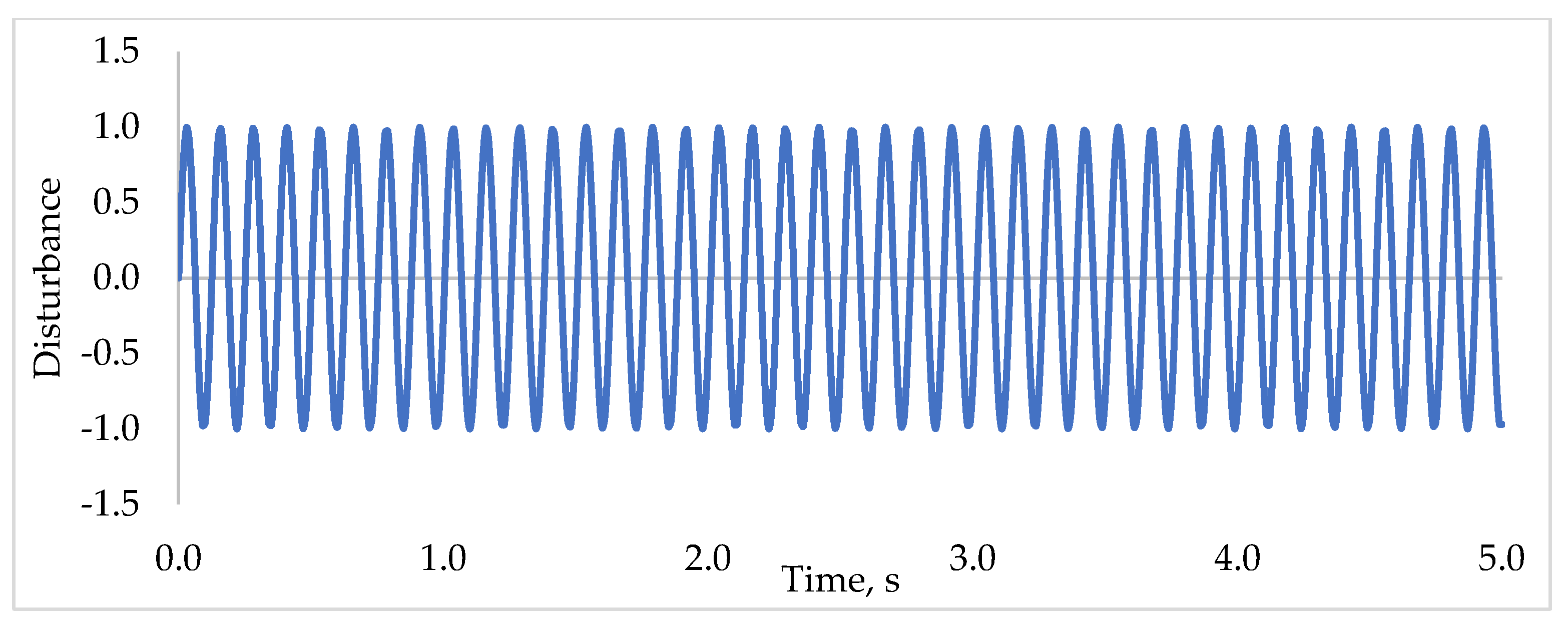
In the first test, it is assumed that the quadrotor is flying in an environment where it was constantly subjected to an unknown external disturbance throughout the flight time. The external disturbance force used for the simulation was modeled using a sinusoidal wave function with the amplitude of 1 and the frequency of 8 Hz, as shown in Equation (14). The use of this type of wind gust profile is because according to [55], this type of wind gust profile and step gust profile occurs relatively often in nature. Both step and sinusoidal functions can be used to construct an arbitrary wind gust profile. The choice of the amplitude and the frequency of the modeled disturbance were based on various researchers’ work, as shown in

Table A5. Review of Sinusoidal wind gust profile.

References	Sinusoidal Wind Gust Profile
	Amplitude	Frequency
Yang and Yan [70]	0.002–0.01	π/100
Khebbache and Tadjine [71]	0.004–0.008	0.1
Razmi and Afshinfar [72]	0.01	0.01
Dong and He [73]	0.1–0.15	0.1π
Barikbin and Fakharian [56]	0.1–0.2	0.3–0.5
Alkamachi and Erçelebi [74]	0.2	0.5
Li, Ma [75]	0.2	1.5–2
Doukhi and Lee [49]	0.8	0.6
Zhen, Qi [76]	1	1
Nadda and Swarup [77]	1	2
Budiyono, Kang [78]	1	≈0.16
Luque-Vega, Castillo-Toledo [79]	1	0.1
Ru and Subbarao [80]	1	10
Fethalla, Saad [81]	1–2.5	0.1–4
Wang and Chen [82]	10–60	1.2–3
Ha and Hong [83]	(3t + 5), (2t)	1–2

in the Appendix C. Based on Table A5, we can see that the amplitude and frequency used were as low as 0.002 and π/100, respectively, while the highest values were up to 60 and 10, respectively. Therefore, an amplitude of 1 and 8 Hz frequency have been chosen for this work, which is within the prescribed ranges mentioned earlier. This model is sufficient to be used for approximating the external disturbance face by the quadrotor [49,56]. The external disturbance was injected into both the altitude and attitude subsystem. The plot of the disturbance’s model is presented in Figure 9.

d(t) = 1sin(8t)

(14)

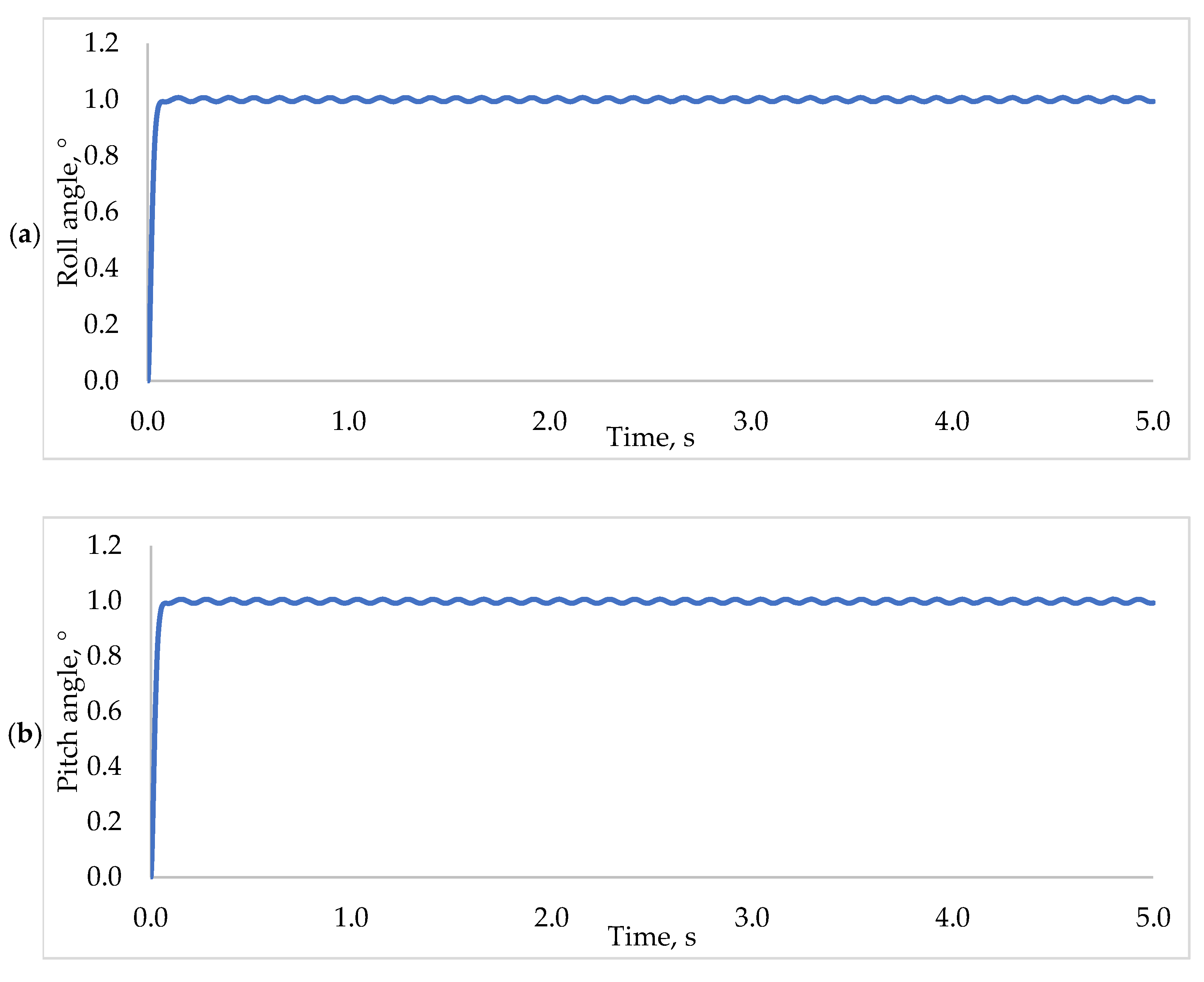
The step response of the system using the proposed REA based PD2-LQR controller subjected to the unknown external disturbance are shown in Figure 10a–d, for the roll, pitch, yaw, and altitude motion respectively.

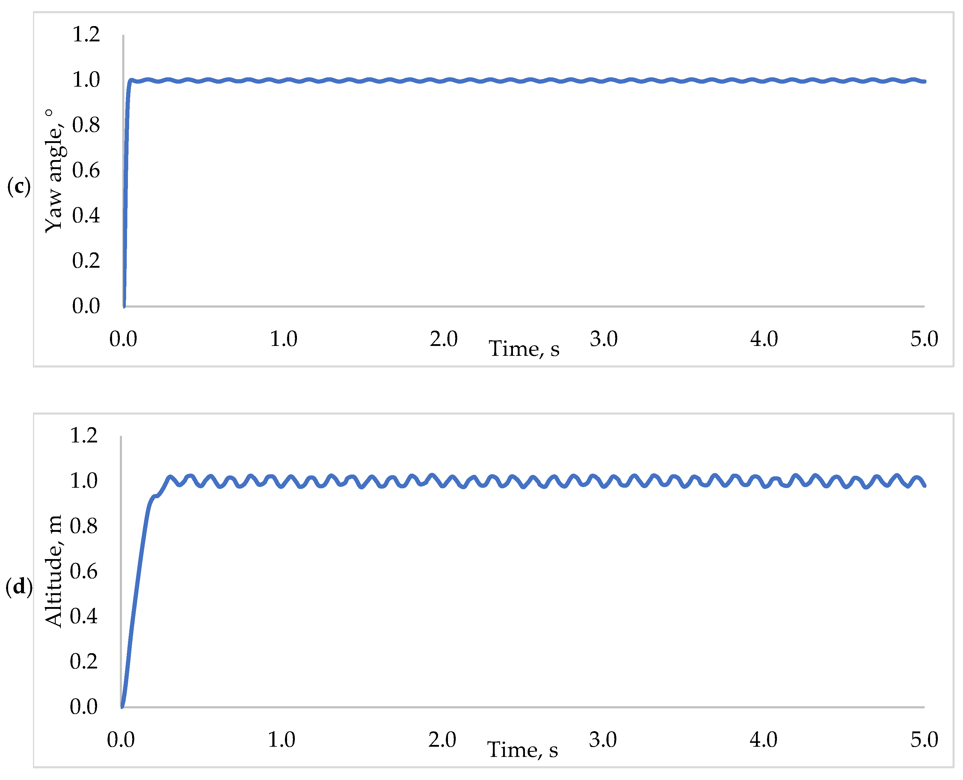
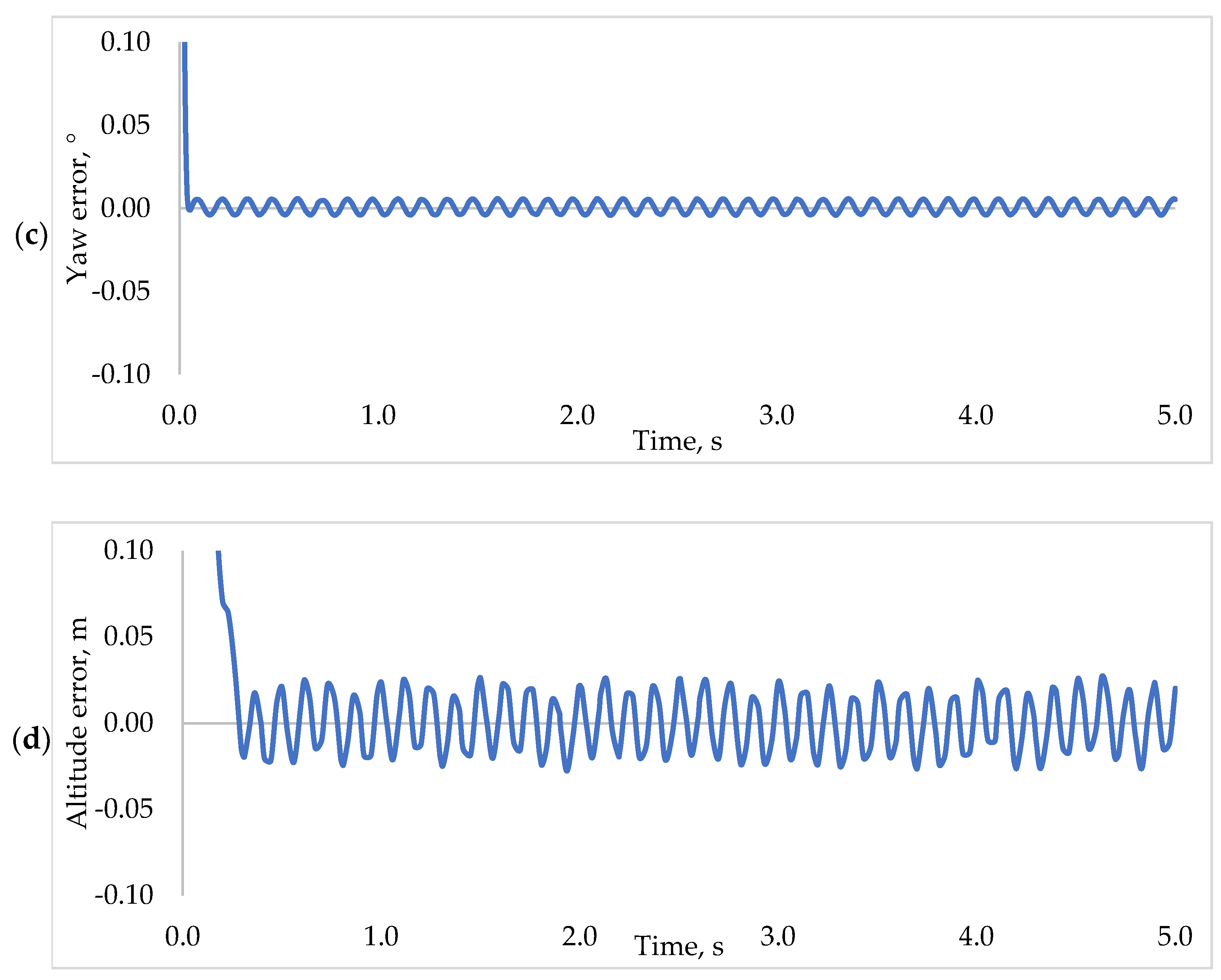
From these figures, it is observed that there is a little bit of attenuation in the system’s response around the desired reference point. This attenuation occurs because of the time-varying disturbance that we have defined earlier. However, the controller could still control and stabilize the quadrotor within the desired reference altitude and angle without any severe degradation in its performance. Suppose we can see from the altitude and attitude error response of the system in Figure 11. In that case, the error produced is not too significant, and the deviation is only around ±0.01° for roll, pitch, and yaw motion, respectively, and ±0.03 m for the altitude motion.

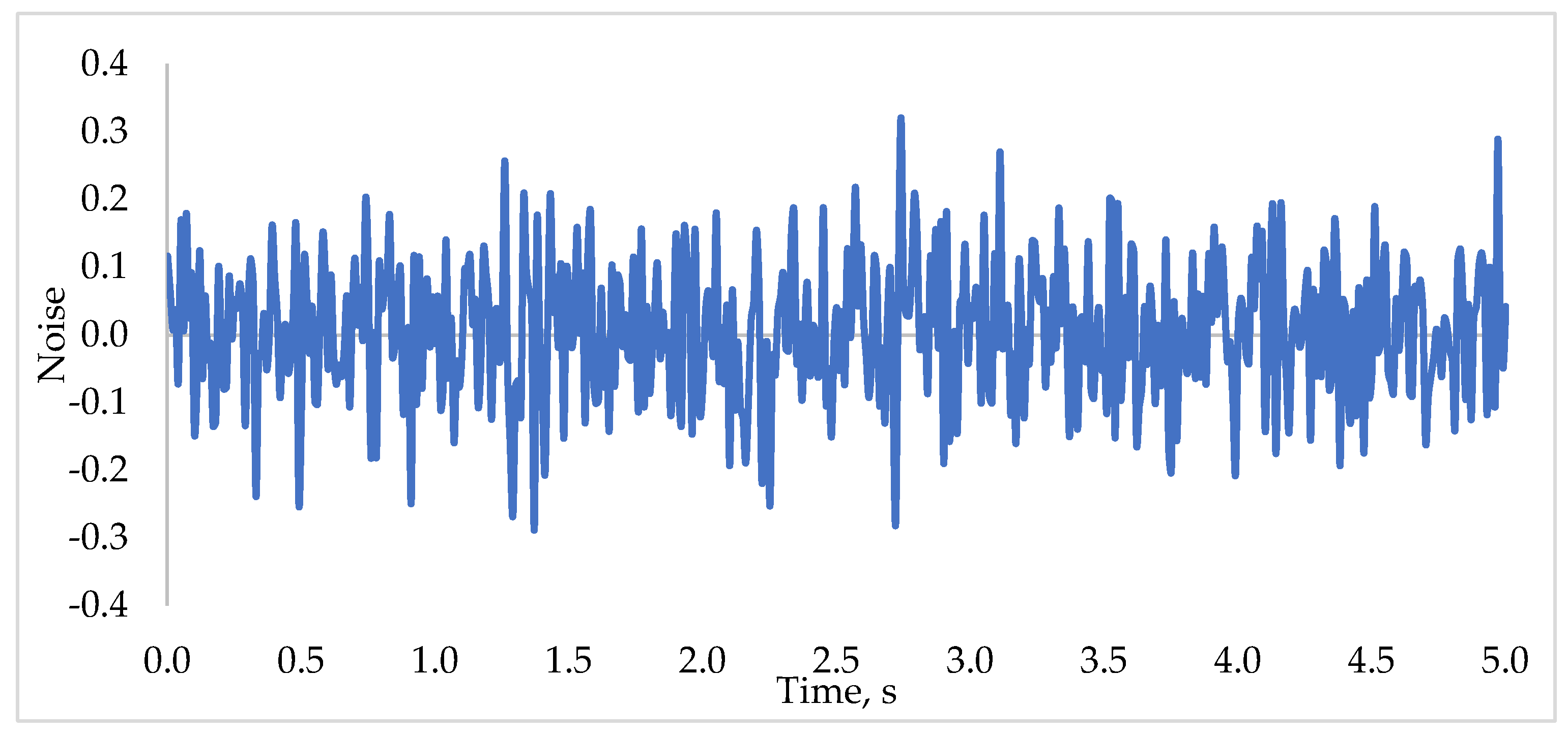
In the second test, we assume that the system is contaminated with the noisy signal coming back from the feedback loop sensor. White Gaussian noise with a zero mean value and variance of 0.01 was applied [57] to simulate the sensor noise present in the feedback signal. The generated noise was fed into the feedback loop for both the altitude and attitude subsystems. The plot for the generated sensor noise is presented in Figure 12.

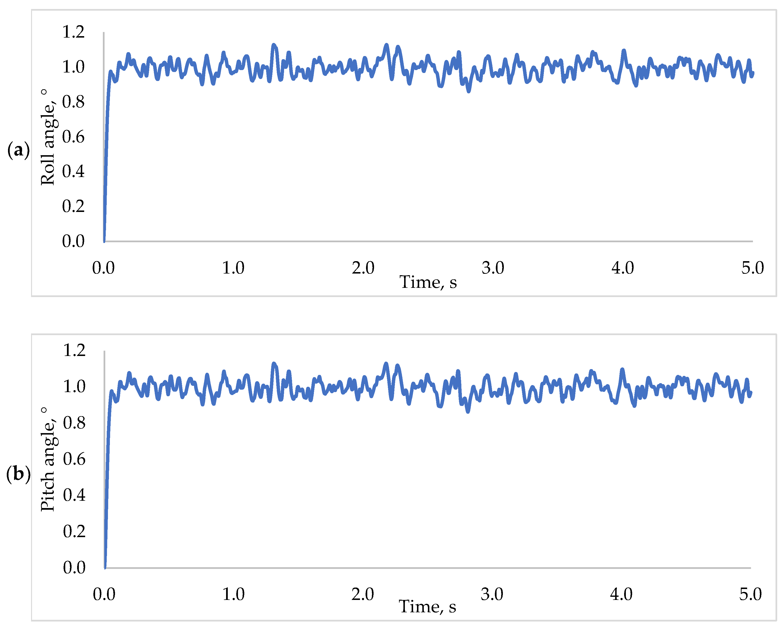
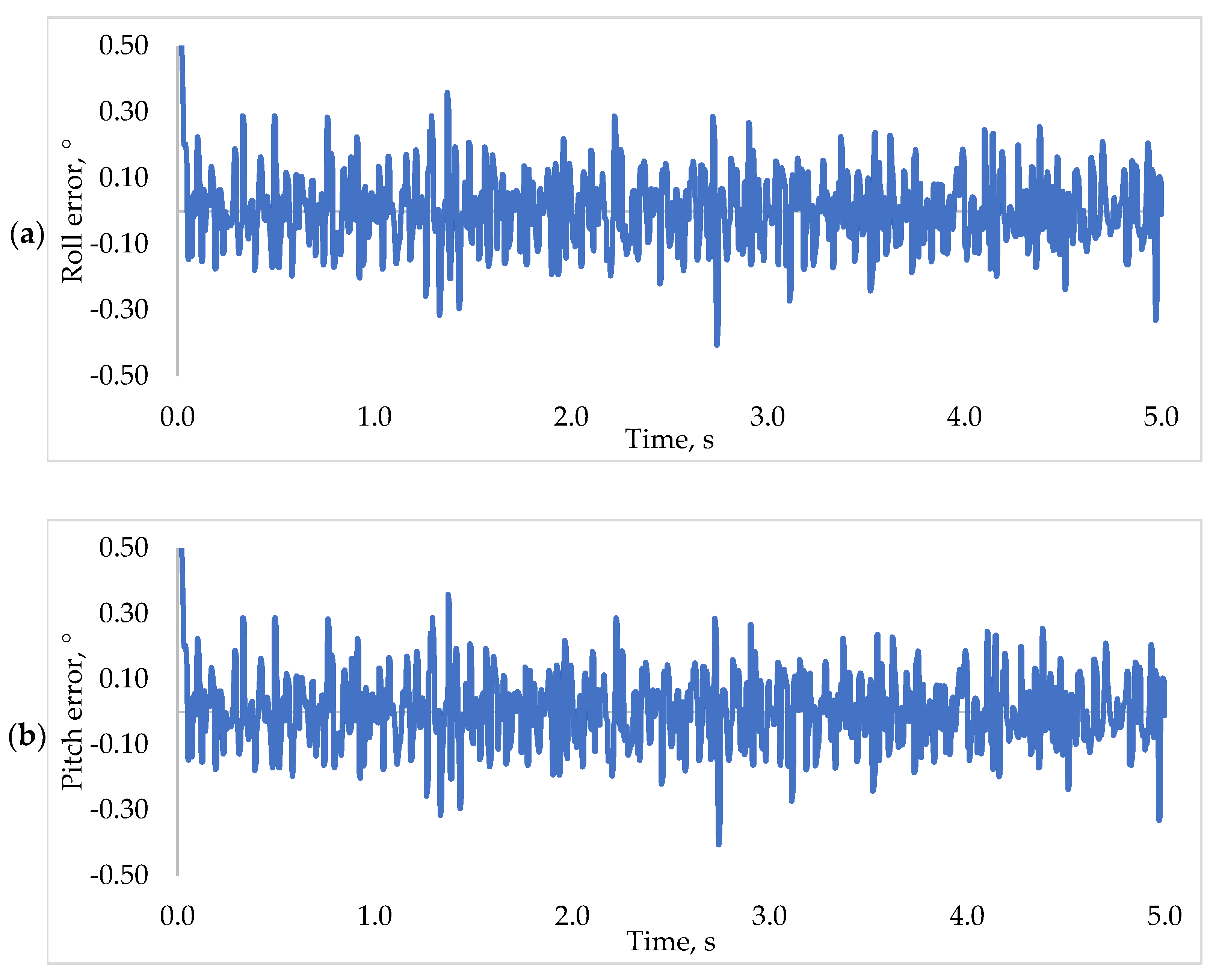
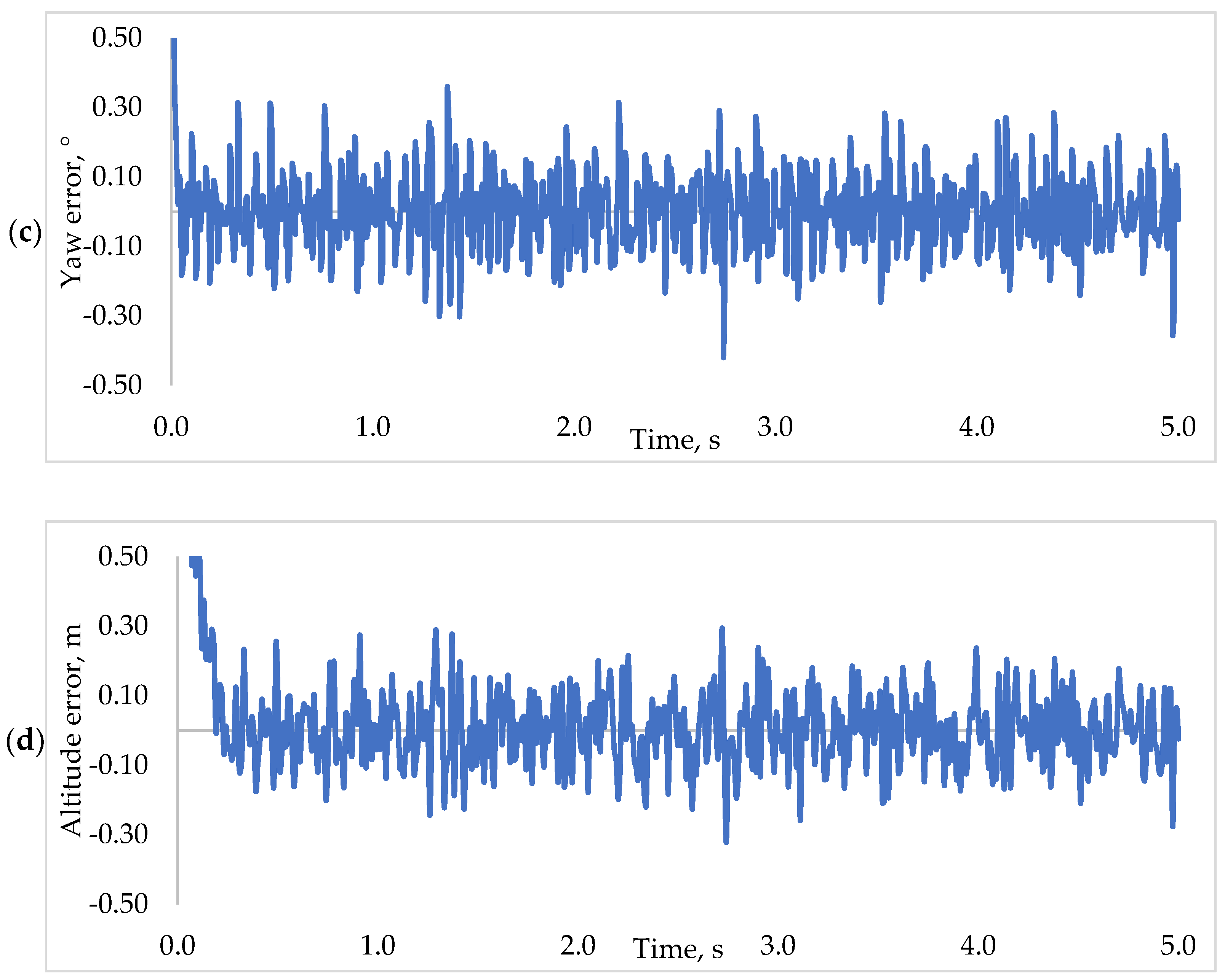
The step responses of the system using the proposed REA based PD2-LQR controller subjected to the sensor noise present in the system are shown in Figure 13a–d for the roll, pitch, yaw, and altitude motion respectively. From these figures, it is observed that the system is a little bit attenuating around the desired reference point since it was constantly exposed to the sensor noise. Nonetheless, the controller could still control and stabilize the quadrotor within the desired reference altitude and angle without a significant deterioration in its performance. Suppose we can see from the altitude and attitude error response of the system in Figure 14. In that case, the error produced is not too large, and the deviation is only around ±0.3° for roll, pitch, and yaw motion, respectively, and also ±0.3 m for the altitude motion.

5.5. Summary

In the previous subsections, the simulation result of the controllers in all four motions, roll, pitch, yaw, and altitude has been presented and discussed. In the first subsection, a comparative study between the proposed algorithm, REA, with eight well-known algorithms like PSO, ABC, GA, DE, MVO, MFO, FA, and STOA has been made in order to demonstrate the effectiveness of the propose algorithm over other algorithms in terms of the exploitation and exploration capability, convergence speed, and the accuracy of the algorithm in finding the optimal solution. The results show that REA delivered a very competitive result compared to the eight other well-known metaheuristic algorithms such as PSO, ABC, GA, DE, MVO, MFO, FA, and STOA.

Next, after we found that the proposed algorithm can provide a satisfactory performance compared to other algorithms when tested on the 23 benchmark test functions as provided in Appendix A, we then implemented all of the algorithm on the proposed PD2-LQR controller. Similarly, a comparative study between the proposed REA PD2-LQR controller and other algorithms based PD2-LQR controller has been conducted. The performance of the controllers was evaluated based on the rise time, settling time, percentage overshoot, steady-state error, and RMSE of the system’s response. Based on the findings, we can realize that the proposed controller can give a superior performance than the other controller. Moreover, the proposed algorithm can provide an optimal solution for the controller’s parameters which led to a better system’s response.

The rise time produce by the REA based controller is 0.03361 s, 0.03361 s, 0.02294 s, and 0.15748 s in roll, pitch, yaw, and altitude motion, respectively, with the settling time of 0.05713 s (roll/pitch), 0.03742 s (yaw), and 0.26129 s (altitude). The REA based controller produced no overshoot in all four motions (0%). However, it is worth noting that some other controllers like PSO, ABC, GA, DE, MVO, FA, and STOA based controller also produce no overshoot in roll and pitch motion, PSO, ABC, GA, MVO, FA, and STOA based controller in yaw motion, and ABC, GA, DE, and MFO based controller in altitude motion.

Concerning the steady-state error, the proposed REA based controller only has the best performance in roll and pitch motion with an error of 6.44466E-06, respectively. In contrast, in the yaw and altitude motion, it was dominated by MFO based controller with 9.20977E-05 and FA based controller with 1.92583E-11, respectively. In terms of RMSE, MVO based controller outperformed REA based controller in roll, pitch, and altitude motion with 0.21630, 0.21630, and 0.39700, respectively, while DE based controller in yaw motion with 0.16930.

On evaluating the worst performance, it is observed that in terms of the rise time, GA and DE based controller is the worst with 0.10570 s in roll/pitch motion, and 0.16879s in altitude motion for GA based controller, while 0.11720 s in yaw motion for DE based controller. In addition, the same controller also has the worst settling time with 0.19360s in roll/pitch motion (GA), 0.28837 s in altitude motion (GA), and 0.21080s in yaw motion (DE). The highest overshoot is produced by MFO based controller with 2.32631E-02%, 2.32631E-02%, and 1.55229E-02% in roll, pitch, and yaw motion, while STOA based controller is the highest in the altitude motion with 1.52380E-04%.

As to steady-state error, it is found that PSO based controller has the highest error in roll (3.20000E-03), pitch (3.20000E-03), and yaw (2.40000E-03), respectively while DE is the highest in altitude motion with an error of 1.92650E-04. Lastly, in RMSE, ABC, REA, and GA based controllers produce the highest error in roll/pitch, yaw, and altitude, respectively. These values are 0.24068 (ABC)(roll/pitch), 0.20431 (REA)(yaw), and 0.40447 (GA)(altitude). If we can notice that the RMSE of the proposed REA based controller is the worst in yaw motion, the highest difference is only 0.03501 with the best controller, which is very minimal; thus, it can still be accepted.

Finally, in order to test the robustness of the proposed controller, a simulation with the present of the unknown external disturbance such as wind gust and sensor noise was conducted to simulate the real-world condition. The external disturbance was modeled using a sinusoidal wave function with the amplitude of 1 and a frequency of 8Hz. The sensor noise was modeled using white Gaussian noise with a zero mean value and variance of 0.01. The external disturbance and the sensor noise were applied for the simulation period. The simulation result shows that the proposed controller can still work effectively even under these condition with minimal error produce.

This study only conducted a simulation work to prove the REA PD2-LQR controller’s superior performance. According to several studies that compare simulation and experimental work, it is found that the performance has some differences when a real implementation is done. Still, the differences between these two works are not too significant. Therefore, we present some references that work on simulation and experimental study of the quadrotor control and stabilization to support our findings further.

Raza and Gueaieb [51] presented their findings that the pitch and roll angle are within (−3, +4)° for simulation, while (−8, +7) and (−6, +12)° in pitch and roll, respectively, for experimental work. Li and Li [58] found that the quadrotor’s attitude angle fluctuated at ±5° from a 0.1° reference angle. In work done by Burggräf, Pérez Martínez [52], the stabilization time for the attitude angle is around 1.3 s for simulation, while for an experiment, it takes 2.2 s to stabilized. Rich and Elia’s [53] results show that simulation and experimental work is almost the same, with approximately less than 10 s to settle at the desired altitude. Hong and Nguyen [54] did the position control of the quadrotor using a gain-scheduling PD controller. They found that the time taken to reach the desired reference is 9.55 s for simulation while 17.5 s for experimental.

Fang and Gao [59] found that all the attitude angles are within ±0.1 radian and the steady-state error of the altitude is ≈0 for the simulation, while the experimental results show that the attitude is almost the same as the simulation, which is also within ±0.1 radian and the altitude has maximum 5 cm deviation. Mohammadi and Shahri [60] found that all the attitude angles are within ≈±1°. The steady-state error of the altitude is within ≈0.1 m for the simulation. At the same time, the experimental results show that the roll angle is within ≈(+2, −1)°, the pitch, and yaw angle is within ≈(+1.5, −1)°, and the altitude is within ≈(−0.03, +0.04) meter.

In Tan and Lu [61], findings show that the roll and pitch angles are stabilized within ≈0°, and the yaw angle is within ≈±0.05° for the simulation, while the experimental results show that the roll and pitch angles are stabilized within ±1°, and the yaw angle is within ±3°. Kim and Nguyen [62] presented findings which show that all the attitude angles are stabilized within ≈0 radians for the simulation, while the experimental result shows that the roll angle is stabilized within ≈±0.02 radian, the pitch angle is within ≈±0.05 radian, and the yaw angle is less than ≈0.1 radian.

Abbasi [63] presented that all the attitude angle are stabilized within ≈0 radians for the simulation, while the experimental results show that the roll angle is stabilized within less than ≈±5° (0.09 radian) and the pitch angle is within less than ≈±3° (0.05 radian). In Xuan-Mung and Hong [64], the altitude error converges to zero within ≈21 s after step input is commanded at 5 s for the simulation. The experimental results show that the quadrotor reaches the desired altitude within ≈45 s after step input is commanded at 10 s. There is a 19 s difference between the simulation and experiment.

In Martins and Cardeira [65], the root mean square error of the x/y/z position and yaw angle are 0.0865 m, 0.0714 m, 0.0556 m, and 0.0095° respectively for the simulation, while the experimental results are 0.1010 m, 0.0781 m, 0.0570 m, and 0.2244° respectively. Wu and Hu [66] presented that all the attitude angles are stabilized within ≈0 radians for the simulation. Simultaneously, the experimental results show that the roll angle is stabilized within less than ≈(+0.4, −0.3) radian, the pitch angle is within less than ≈(+0.1, −0.5) radian. The yaw angle is less than ≈±4 radian.

Choi and Ahn [67], found that the position and attitude angle are stabilized within ≈0 m and degree error respectively for the simulation, while the experimental result show that the x/y position has maximum peak error of less than ≈1.5 m, the altitude error is less than 0.1 m, the roll angle is stabilized within less than ≈(+3, −5)°, and the pitch angle is within less than ≈±0.3°. Lu and Liu [68] found the quadrotor successfully tracks the desired trajectory with almost zero tracking error for the simulation. Simultaneously, the experimental results show tracking error is produced but still within the acceptable range.

Feng [69] found that the roll and pitch angles are stabilized within ≈0 radians for the simulation, while the experimental results show that the roll and pitch angles are stabilized within less than ≈±0.05 and ≈±0.02 radians respectively. In summary, based on these references that work on both simulation and experimental studies, we can conclude that the deviation between the performance in simulation and experiment is not too significant or too severe. Hence, when the proposed controller based on a simulation work implemented on a real platform, it can still be stable even with marginal degrees/meters of error.

6. Conclusions

This paper presented an optimization algorithm called a Random Explosion Algorithm (REA). This algorithm’s fundamental idea is based on a simple concept of an explosion that will produce a randomly dispersed fragment around the initial particle within the explosion radius when a particle is exploded. The algorithm was tested on the 23 benchmark test functions to evaluate the algorithm’s performance in exploration, exploitation, local optima avoidance, and convergence behavior. The results show that REA delivered a very competitive result compared to the eight other well-known metaheuristic algorithms such as PSO, ABC, GA, DE, MVO, MFO, FA, and STOA. About the first benchmark functions (unimodal benchmark functions), REA has a superior exploitation capability to exploit the optimum value of the functions. The second benchmark functions (multimodal and fixed dimensional multimodal benchmark functions) have confirmed that REA could explore the promising region in the search space and escape the local optima and seek the global optimum. The convergence analysis has proved that the REA could converge faster and accurately toward the global optimum than the other algorithms. Besides that, we also implemented the algorithm for the quadrotor control application. The proposed REA based controller’s performance in terms of the rise time, settling time, percentage overshoot, steady-state error, and RMSE of a system’s response has been compared and evaluated with the other optimization-based controller stated before. The simulation result shows that the proposed REA based controller gives the best control performance in terms of the rise time, settling time, and percentage overshoot in all four motions (roll, pitch, yaw, altitude), while producing small steady-state error and RMSE as other controller. Finally, the proposed controller’s robustness test has also been conducted to simulate the real-world application where the quadrotor is always subjected to an unknown external disturbance and suffers from the sensor noise coming from the mechanical vibration in the electronic part. The external disturbance was modeled using the sinusoidal wave function with an amplitude of 1 and a frequency of 8 Hz. The sensor noise was modeled using white Gaussian noise with a zero mean value and variance of 0.01. Under this set of conditions, the simulation result shows that the proposed controller can still work effectively with only minimal error produces. The errors are ±0.01° for the roll, pitch, and yaw motion and ±0.03 m for the altitude motion under the presence of external disturbance, while ±0.3 degrees/meters in all four motion when subjected to the sensor noise. In conclusion, based on these findings, we can say that the proposed REA algorithm and REA based controller are suitable and can be used for the controller’s parameter tuning and quadrotor control and stabilization. More so since it can provide a further improvement to the quadrotor’s system performance in all four motion with an excellent overall result.

References

- Mirjalili, S.; Mirjalili, S.M.; Lewis, A. Grey Wolf Optimizer. Adv. Eng. Softw. 2014, 69, 46–61. [Google Scholar] [CrossRef] [Green Version]
- Dhiman, G.; Kumar, V. Emperor penguin optimizer: A bio-inspired algorithm for engineering problems. Knowl. Based Syst. 2018, 159, 20–50. [Google Scholar] [CrossRef]
- Dhiman, G.; Kumar, V. Spotted hyena optimizer: A novel bio-inspired based metaheuristic technique for engineering applications. Adv. Eng. Softw. 2017, 114, 48–70. [Google Scholar] [CrossRef]
- Holland, J.H. Genetic algorithms. Sci. Am. 1992, 267, 66–73. [Google Scholar] [CrossRef]
- Storn, R.; Price, K. Differential Evolution–A Simple and Efficient Heuristic for global Optimization over Continuous Spaces. J. Glob. Optim. 1997, 11, 341–359. [Google Scholar] [CrossRef]
- Rechenberg, I. Evolutionsstrategien, in Simulationsmethoden in der Medizin und Biologie; Springer: Berlin/Heidelberg, Germany, 1978; pp. 83–114. [Google Scholar]
- Beyer, G.H.P.; Schwefel, H. Evolution strategies–A comprehensive introduction. Nat. Comput. 2002, 1, 3–52. [Google Scholar] [CrossRef]
- Koza, R.J.; Koza, J.R. Genetic Programming: On the Programming of Computers by Means of Natural Selection; MIT Press: Cambridge, MA, USA, 1992; Volume 1. [Google Scholar]
- Simon, D. Biogeography-Based Optimization. IEEE Trans. Evol. Comput. 2008, 12, 702–713. [Google Scholar] [CrossRef] [Green Version]
- Kirkpatrick, S.; Gelatt, C.D., Jr.; Vecchi, M.P. Optimization by simulated annealing. Science 1983, 220, 671–680. [Google Scholar] [CrossRef]
- Rashedi, E.; Nezamabadi-pour, H.; Saryazdi, S. GSA: A Gravitational Search Algorithm. Inf. Sci. 2009, 179, 2232–2248. [Google Scholar] [CrossRef]
- Hatamlou, A. Black hole: A new heuristic optimization approach for data clustering. Inf. Sci. 2013, 222, 175–184. [Google Scholar] [CrossRef]
- Kaveh, A.; Khayatazad, M. A new meta-heuristic method: Ray Optimization. Comput. Struct. 2012, 112–113, 283–294. [Google Scholar] [CrossRef]
- Erol, K.O.; Eksin, I. A new optimization method: Big Bang–Big Crunch. Adv. Eng. Softw. 2006, 37, 106–111. [Google Scholar] [CrossRef]
- Formato, R.A. Central force optimization: A new deterministic gradient-like optimization metaheuristic. OPSEARCH 2009, 46, 25–51. [Google Scholar] [CrossRef]
- Kaveh, A.; Talatahari, S. A novel heuristic optimization method: Charged system search. Acta Mech. 2010, 213, 267–289. [Google Scholar] [CrossRef]
- Du, H.; Wu, X.; Zhuang, J. Small-World Optimization Algorithm for Function Optimization. In Advances in Natural Computation; Springer: Berlin/Heidelberg, Germany, 2006. [Google Scholar]
- Alatas, B. ACROA: Artificial Chemical Reaction Optimization Algorithm for global optimization. Expert Syst. Appl. 2011, 38, 13170–13180. [Google Scholar] [CrossRef]
- Shah-Hosseini, H. Principal components analysis by the galaxy-based search algorithm: A novel metaheuristic for continuous optimisation. Int. J. Comput. Sci. Eng. 2011, 6, 132–140. [Google Scholar]
- Moghaddam, F.F.; Moghaddam, R.F.; Cheriet, M. Curved space optimization: A random search based on general relativity theory. arXiv 2012, arXiv:1208.2214. Available online: https://arxiv.org/pdf/1208.2214.pdf (accessed on 24 April 2021).
- Kennedy, J.; Eberhart, R. Particle Swarm Optimization. In Proceedings of the ICNN’95—International Conference on Neural Networks, Perth, Western Australia, 27 November–1 December 1995. [Google Scholar]
- Dorigo, M.; Birattari, M.; Stützle, T. Ant Colony Optimization: Artificial Ants as a Computational Intelligence Technique. IEEE Comput. Intell. Mag. 2006, 1, 28–39. [Google Scholar] [CrossRef] [Green Version]
- Karaboga, D.; Basturk, B. A powerful and efficient algorithm for numerical function optimization: Artificial bee colony (ABC) algorithm. J. Glob. Optim. 2007, 39, 459–471. [Google Scholar] [CrossRef]
- Mucherino, A.; Seref, O. Monkey Search: A Novel Metaheuristic Search for Global Optimization. In AIP Conference Proceedings; American Institute of Physics: College Park, MA, USA, 2007. [Google Scholar]
- Yang, X.; Suash, D. Cuckoo Search via Lévy Flights. In Proceedings of the 2009 World Congress on Nature & Biologically Inspired Computing (NaBIC), Coimbatore, India, 9–11 December 2009. [Google Scholar]
- Yang, X.-S. A New Metaheuristic Bat-Inspired Algorithm. In Nature Inspired Cooperative Strategies for Optimization (NICSO 2010); González, J.R., Pelta, D.A., Cruz, C., Terrazas, G., Krasnogor, N., Eds.; Springer: Berlin/Heidelberg, Germany, 2010; pp. 65–74. [Google Scholar]
- Shiqin, Y.; Jianjun, J.; Guangxing, Y. A Dolphin Partner Optimization. In Proceedings of the 2009 WRI Global Congress on Intelligent Systems, Xiamen, China, 19–21 May 2009. [Google Scholar]
- Yang, X.-S. Firefly algorithm, stochastic test functions and design optimisation. Int. J. Bio-Inspired Comput. 2010, 2, 78–84. [Google Scholar] [CrossRef]
- Lu, X.; Zhou, Y. A Novel Global Convergence Algorithm: Bee Collecting Pollen Algorithm. In Advanced Intelligent Computing Theories and Applications. With Aspects of Artificial Intelligence; Springer: Berlin/Heidelberg, Germany, 2008. [Google Scholar]
- Abbass, H.A. MBO: Marriage in Honey Bees Optimization-A Haplometrosis Polygynous Swarming Approach. In Proceedings of the 2001 Congress on Evolutionary Computation (IEEE Cat. No. 01TH8546), Seoul, Korea, 27–30 May 2001. [Google Scholar]
- Alba, E.; Dorronsoro, B. The exploration/exploitation tradeoff in dynamic cellular genetic algorithms. IEEE Trans. Evol. Comput. 2005, 9, 126–142. [Google Scholar] [CrossRef] [Green Version]
- Olorunda, O.; Engelbrecht, A.P. Measuring Exploration/Exploitation in Particle Swarms Using Swarm Diversity. In Proceedings of the 2008 IEEE Congress on Evolutionary Computation (IEEE World Congress on Computational Intelligence), Hong Kong, 1–6 June 2008. [Google Scholar]
- Lozano, M.; García-Martínez, C. Hybrid metaheuristics with evolutionary algorithms specializing in intensification and diversification: Overview and progress report. Comput. Oper. Res. 2010, 37, 481–497. [Google Scholar] [CrossRef]
- Shanghooshabad, M.A.; Abadeh, M.S. Robust, interpretable and high quality fuzzy rule discovery using krill herd algorithm. J. Intell. Fuzzy Syst. 2016, 30, 1601–1612. [Google Scholar] [CrossRef]
- Ali, F.A.; Tawhid, M.A. Ahybrid cuckoo search algorithm with Nelder Mead method for solving global optimization problems. Springer Plus 2016, 5, 473. [Google Scholar] [CrossRef] [Green Version]
- Baer, K.; Ericson, L.; Krus, P. Robustness and performance evaluations for simulation-based control and component parameter optimization for a series hydraulic hybrid vehicle. Eng. Optim. 2020, 52, 446–464. [Google Scholar] [CrossRef] [Green Version]
- Wolpert, H.D.; Macready, W.G. Nofree lunch theorems for optimization. IEEE Trans. Evol. Comput. 1997, 1, 67–82. [Google Scholar] [CrossRef] [Green Version]
- Shehab, M.; Khader, A.T.; Al-Betar, M.A. A survey on applications and variants of the cuckoo search algorithm. Appl. Soft Comput. 2017, 61, 1041–1059. [Google Scholar] [CrossRef]
- Tangherloni, A.; Spolaor, S.; Cazzaniga, P.; Besozzi, D.; Rundo, L.; Mauri, G.; Nobile, M.S. Biochemical parameter estimation vs. benchmark functions: A comparative study of optimization performance and representation design. Appl. Soft Comput. 2019, 81, 105494. [Google Scholar] [CrossRef]
- Jamil, M.; Yang, X.-S. A literature survey of benchmark functions for global optimisation problems. Int. J. Math. Model. Numer. Optim. 2013, 4, 150–194. [Google Scholar] [CrossRef] [Green Version]
- Yang, S.X.; He, X.-S.; Fan, Q.-W. Chapter 7-Mathematical framework for algorithm analysis. In Nature-Inspired Computation and Swarm Intelligence; Yang, X.S., Ed.; Academic Press: Cambridge, MA, USA, 2020; pp. 89–108. [Google Scholar]
- Digalakis, G.J.; Margaritis, K.G. On benchmarking functions for genetic algorithms. Int. J. Comput. Math. 2001, 77, 481–506. [Google Scholar] [CrossRef]
- Saud, L.; Hasan, A. Design of an Optimal Integral Backstepping Controller for a Quadcopter. J. Eng. 2018, 24, 46. [Google Scholar] [CrossRef]
- Erkol, H.O. Attitude controller optimization of four-rotor unmanned air vehicle. Int. J. Micro Air Veh. 2017, 10, 42–49. [Google Scholar] [CrossRef]
- Thanh, N.H.L.N.; Hong, S.K. Quadcopter Robust Adaptive Second Order Sliding Mode Control Based on PID Sliding Surface. IEEE Access 2018, 6, 66850–66860. [Google Scholar] [CrossRef]
- Mirjalili, S.; Mirjalili, S.M.; Hatamlou, A. Multi-Verse Optimizer: A nature-inspired algorithm for global optimization. Neural Comput. Appl. 2016, 27, 495–513. [Google Scholar] [CrossRef]
- Mirjalili, S. Moth-flame optimization algorithm: A novel nature-inspired heuristic paradigm. Knowl. Based Syst. 2015, 89, 228–249. [Google Scholar] [CrossRef]
- Dhiman, G.; Kaur, A. STOA: A bio-inspired based optimization algorithm for industrial engineering problems. Eng. Appl. Artif. Intell. 2019, 82, 148–174. [Google Scholar] [CrossRef]
- Doukhi, O.; Lee, D.J. Neural Network-based Robust Adaptive Certainty Equivalent Controller for Quadrotor UAV with Unknown Disturbances. Int. J. Control. Autom. Syst. 2019, 17, 2365–2374. [Google Scholar] [CrossRef]
- Tanveer, M.H.; Hazry, D.; Ahmed, S.F.; Joyo, M.K.; Warsi, F.A.; Kamarudin, H.; Wan, K.; Razlan, Z.M.; Shahriman, A.B.; Hussain, A.T. Feedback sensor noise rejection control strategy for quadrotor UAV system. Aip Conf. Proc. 2015, 1660, 070053. [Google Scholar]
- Raza, S.; Gueaieb, W. Intelligent Flight Control of an Autonomous Quadrotor. In Motion Control; Casolo, F., Ed.; INTECH: Rijeka, Croatia, 2010; p. 580. [Google Scholar]
- Burggräf, P.; Martínez, A.R.P.; Roth, H.; Wagner, J. Quadrotors in factory applications: Design and implementation of the quadrotor’s P-PID cascade control system. SN Appl. Sci. 2019, 1, 722. [Google Scholar] [CrossRef] [Green Version]
- Rich, M.; Elia, N.; Jones, P. Design and Implementation of an H∞ Controller for a Quadrotor Helicopter. In Proceedings of the 21st Mediterranean Conference on Control and Automation, Crete, Greece, 25–28 June 2013. [Google Scholar]
- Hong, K.S.; Nguyen, N.P. Position control of a hummingbird quadcopter augmented by gain scheduling. Int. J. Eng. Res. Technol. 2018, 11, 1485–1498. [Google Scholar]
- Nelson, R.C. Flight Stability and Automatic Control, 2nd ed.; McGraw Hill: New York, NY, USA, 1998. [Google Scholar]
- Barikbin, B.; Fakharian, A. Trajectory tracking for quadrotor UAV transporting cable-suspended payload in wind presence. Trans. Inst. Meas. Control 2018, 41, 1243–1255. [Google Scholar] [CrossRef]
- Guo, Y.; Jiang, B.; Zhang, Y. A novel robust attitude control for quadrotor aircraft subject to actuator faults and wind gusts. IEEE/CAA J. Autom. Sin. 2018, 5, 292–300. [Google Scholar] [CrossRef]
- Li, J.; Li, Y. Dynamic Analysis and PID Control for a Quadrotor. In Proceedings of the 2011 IEEE International Conference on Mechatronics and Automation, Beijing, China, 7–10 August 2011. [Google Scholar]
- Fang, Z.; Gao, W. Adaptive backstepping control of an indoor micro-quadrotor. Res. J. Appl. Sci. Eng. Technol. 2012, 4, 4216–4226. [Google Scholar]
- Mohammadi, M.; Shahri, A.M. Adaptive Nonlinear Stabilization Control for a Quadrotor UAV: Theory, Simulation and Experimentation. J. Intell. Robot. Syst. 2013, 72, 105–122. [Google Scholar] [CrossRef]
- Tan, L.; Lu, L.; Jin, G. Attitude stabilization control of a quadrotor helicopter using integral backstepping. Iet Conf. Proc. 2012, 573–577. [Google Scholar]
- Kim, G.B.; Nguyen, T.K.; Budiyono, A.; Park, J.K.; Yoon, K.J.; Shin, J. Design and Development of a Class of Rotorcraft-Based UAV. Int. J. Adv. Robot. Syst. 2013, 10, 131. [Google Scholar] [CrossRef] [Green Version]
- Abbasi, E. Development and Implementation of a Adaptive Fuzzy Control System for a VTOL Vehicle in Hovering Mode. Int. J. Control Theory Comput. Modeling 2017, 7, 1–14. [Google Scholar] [CrossRef]
- Xuan-Mung, N.; Hong, S.-K. Improved Altitude Control Algorithm for Quadcopter Unmanned Aerial Vehicles. Appl. Sci. 2019, 9, 2122. [Google Scholar] [CrossRef] [Green Version]
- Martins, L.; Cardeira, C.; Oliveira, P. Linear Quadratic Regulator for Trajectory Tracking of a Quadrotor. Ifac Pap. Online 2019, 52, 176–181. [Google Scholar] [CrossRef]
- Wu, Y.; Hu, K.; Sun, X. Modeling and Control Design for Quadrotors: A Controlled Hamiltonian Systems Approach. IEEE Trans. Veh. Technol. 2018, 67, 11365–11376. [Google Scholar] [CrossRef]
- Choi, Y.; Ahn, H. Nonlinear Control of Quadrotor for Point Tracking: Actual Implementation and Experimental Tests. IEEE/ASME Trans. Mechatron. 2015, 20, 1179–1192. [Google Scholar] [CrossRef]
- Lu, H.; Liu, C.; Coombes, M.; Guo, L.; Chen, W. Online optimisation-based backstepping control design with application to quadrotor. IET Control Theory Appl. 2016, 10, 1601–1611. [Google Scholar] [CrossRef] [Green Version]
- Feng, B. Robust Control for Lateral and Longitudinal Channels of Small-Scale Unmanned Helicopters. J. Control Sci. Eng. 2015, 2015, 483096. [Google Scholar] [CrossRef] [Green Version]
- Yang, Y.; Yan, Y. Attitude regulation for unmanned quadrotors using adaptive fuzzy gain-scheduling sliding mode control. Aerosp. Sci. Technol. 2016, 54, 208–217. [Google Scholar] [CrossRef]
- Khebbache, H.; Tadjine, M. Robust fuzzy backstepping sliding mode controller for a quadrotor unmanned aerial vehicle. J. Control Eng. Appl. Inform. 2013, 15, 3–11. [Google Scholar]
- Razmi, H.; Afshinfar, S. Neural network-based adaptive sliding mode control design for position and attitude control of a quadrotor UAV. Aerosp. Sci. Technol. 2019, 91, 12–27. [Google Scholar] [CrossRef]
- Dong, J.; He, B. Novel Fuzzy PID-Type Iterative Learning Control for Quadrotor UAV. Sensors 2019, 19, 24. [Google Scholar]
- Alkamachi, A.; Erçelebi, E. H∞ control of an overactuated tilt rotors quadcopter. J. Cent. South Univ. 2018, 25, 586–599. [Google Scholar] [CrossRef]
- Li, Z.; Ma, X.; Li, Y. Robust tracking control strategy for a quadrotor using RPD-SMC and RISE. Neurocomputing 2019, 331, 312–322. [Google Scholar] [CrossRef]
- Zhen, H.; Qi, X.; Dong, H. An adaptive block backstepping controller for attitude stabilization of a quadrotor helicopter. WSEAS Trans. Syst. Control 2013, 8, 46–55. [Google Scholar]
- Nadda, S.; Swarup, A. Improved Quadrotor Altitude Control Design Using Second-Order Sliding Mode. J. Aerosp. Eng. 2017, 30, 04017065. [Google Scholar] [CrossRef]
- Budiyono, A.; Kang, T.; Dharmayanda, H.R. State space identification and implementation of H∞ control design for small-scale helicopter. Aircr. Eng. Aerosp. Technol. 2010, 82, 340–352. [Google Scholar]
- Luque-Vega, L.; Castillo-Toledo, B.; Loukianov, A.G. Robust block second order sliding mode control for a quadrotor. J. Frankl. Inst. 2012, 349, 719–739. [Google Scholar] [CrossRef]
- Ru, P.; Subbarao, K. Nonlinear Model Predictive Control for Unmanned Aerial Vehicles. Aerospace 2017, 4, 31. [Google Scholar] [CrossRef]
- Fethalla, N.; Saad, M.; Michalska, H.; Ghommam, J. Robust Observer-Based Dynamic Sliding Mode Controller for a Quadrotor UAV. IEEE Access 2018, 6, 45846–45859. [Google Scholar] [CrossRef]
- Wang, H.; Chen, M. Trajectory tracking control for an indoor quadrotor UAV based on the disturbance observer. Trans. Inst. Meas. Control 2015, 38, 675–692. [Google Scholar] [CrossRef]
- Ha, L.N.; Hong, S.K. Robust Dynamic Sliding Mode Control-Based PID–Super Twisting Algorithm and Disturbance Observer for Second-Order Nonlinear Systems: Application to UAVs. Electronics 2019, 8, 760. [Google Scholar] [CrossRef] [Green Version]
Figure 1.
Classification of metaheuristic algorithms.
Figure 2.
Flowchart of the proposed REA.
Figure 3.
The 3D version of unimodal benchmark functions: reprinted from [3].
Figure 4.
The 3D version of multimodal benchmark function: reprinted from [3].
Figure 5.
The 3D version of fixed dimension multimodal benchmark functions: reprinted from [3].
Figure 6.
The structure of the hybrid PD2-LQR controller.
Figure 7.
Comparison of the convergence curve of REA with other algorithms for various benchmark functions.
Figure 8.
Comparison of the step response, (a) roll, (b) pitch, (c) yaw, and (d) altitude.
Figure 9.
Unknown external disturbance variation over time.
Figure 10.
The step response of the system in the presence of unknown external disturbance, (a) roll, (b) pitch, (c) yaw, and (d) altitude motion.
Figure 11.
The error response of the system in the presence of unknown external disturbance, (a) roll, (b) pitch, (c) yaw, and (d) altitude motion.
Figure 12.
Sensor noise signal.
Figure 13.
The step response of the system in the presence of sensor noise, (a) roll, (b) pitch, (c) yaw, and (d) altitude motion.
Figure 14.
The error response of the system in the presence of sensor noise, (a) roll, (b) pitch, (c) yaw, and (d) altitude motion.