
The Use of Machine Learning for the Prediction of the Uniformity of the Degree of Cure of a Composite in an Autoclave

School of Aeronautic Science and Engineering, Beihang University (BUAA), Beijing 100191, China
*
Author to whom correspondence should be addressed.
Aerospace 2021, 8(5), 130; https://0-doi-org.brum.beds.ac.uk/10.3390/aerospace8050130
Submission received: 15 March 2021
/
Revised: 16 April 2021
/
Accepted: 20 April 2021
/
Published: 5 May 2021
Abstract
:The difference in the degree of cure of the composite in an autoclave is one of the main characterization parameters of the uniformity of the degree of cure of the composite material. Therefore, it is very important to develop an effective method for predicting the difference in the curing degree of a composite autoclave to improve the uniformity of the curing degree of the composite materials. We researched five machine learning models: a fully connected neural network (FCNN) model, a deep neural network (DNN) model, a radial basis function (RBF) neural network model, a support vector regression (SVR) model and a K-nearest neighbors (KNN) model. We regarded the heating rate, holding time and holding temperature of the composite material’s two holding-stage cure profile as input parameters and established a rapid estimation model of the maximum curing degree difference at any time during the molding process. We simulated the molding process of the composite material in an autoclave to obtain the maximum difference in the curing degree as the test sample data to train five machine learning models and compared and verified the different models after the training. The results showed that the RBF neural network model had the best prediction effect among the five models and the RBF was the most suitable algorithm for this model.
1. Introduction
Composite materials have the advantages of high specific strength, high specific stiffness and designability of the mechanical properties of materials. They are ideal materials for lightweight and efficient structural designs. Due to their excellent characteristics, composite materials are widely used in aerospace and military industries. Autoclave forming is one of the most common forming processes, which refers to a process method in which a single layer of pre-preg is stacked in a predetermined direction to place a composite material blank in a thermopressed tank and complete the curing process at a given temperature and pressure. The curing process is a critical stage in the manufacture of composite parts. The final quality of the part depends largely on the curing curve used in the curing process. Due to the exothermic phenomenon and low thermal conductivity of composites, the cure process will considerably lead to a nonuniform degree of cure, which is the major factor that causes the residual stress. Therefore, it is of great significance to study the effect of the curing process curve on the uniformity of the degree of cure of the composite material during the molding process of the composite in an autoclave.
So far, the research on the formation of a composite in an autoclave has mostly been in the simulation and experimental stages. Loos and Springer [1] studied 1D cure simulation and provided a temperature distribution and degree of cure of the resin. Bogetti and Gillespie [2] conducted a two-dimensional (2D) cure simulation for thick thermoset composites using the finite difference method by which the transient anisotropic heat transfer equation coupled with cure kinetics was solved to predict the temperature and degree of cure distributions as a function of the autoclave temperature history. Johnston and Joshi [3] introduced an approach using an implicit FE method to simulate the cure process of 2D laminates. Johnston [4] measured the heat transfer coefficient of the thermal history of three types of autoclaves to predict the temperature field distribution of the autoclave and found that the pressure could significantly improve the uniformity of the temperature field of the autoclave and shorten the thermal history time. Although simulations and experiments can provide good results they consume a lot of time and manpower. In order to solve the above problems, this paper investigates different machine learning models, proposes a prediction method for the uniformity of composite materials in an autoclave forming based on machine learning and trains five models including the fully connected neural network (FCNN) model, the deep neural network (DNN) model, the radial basis function (RBF) neural network model, the support vector regression (SVR) model and the K-nearest neighbors (KNN) model. In this paper, a two holding-stage cure profile is considered; a total of six parameters including two heating rates, and , two holding times, and , and two holding temperatures, and , are chosen to represent the cure profile [5]. Blest [6] studied the resin flow, heat transfer models and simulations of the curing composites in an autoclave and found that the numerical simulation results were considered to be approximately valid compared with the existing test data. Therefore, this paper considers sufficient ABAQUS finite element modelings and analysis results as real data to train, test and verify the five models. “One machine learning algorithm may show optimum performance for the discriminative features of a particular problem but fails for others” [7]. Based on the comparison of the training results, this paper draws the best solution. The innovation of this article lies in the application of traditional machine learning methods to the field of composite materials. These models provide a new and effective method for the estimation of the maximum ∆α of a composite in an autoclave forming.
2. Material Description
The composite material was a thermosetting resin matrix composite material, the reinforcement was an AS4 unidirectional fiber and the matrix was epoxy resin. The manufacturing technology of resin matrix composites largely determines the quality, cost and performance of the composite parts. As a currently widely used composite structure molding process, autoclave molding uses a uniform temperature and pressure provided in the tank for curing and molding. When the autoclave is formed, the composite material blank structure is sealed on the surface of the mold with a vacuum bag and vacuum treatment is performed. After the process of heating, pressurizing, heat preservation, cooling and pressure relief, the part is formed.
In this paper, we established a three-dimensional classic temperature field calculation model in ABAQUS first. According to the calculation model of Cheung [8,9] et al., a flat plate with a thickness of 8 mm, a length of 200 mm and a width of 80 mm was established. The material system was an AS4/3501-6 resin matrix composite material and its curing kinetic model is shown in Equation (1) [10]. The thermodynamic properties and curing kinetic model [11] parameters are shown in Table 1.
where is the degree of cure and are the curing reaction rate constants, which follow the Arrhenius equation.
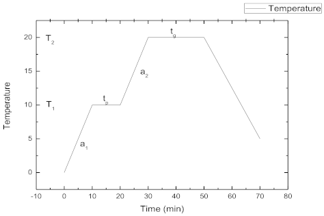
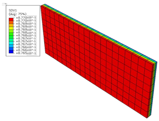
In this paper, according to the subroutine in Gao’s dissertation [11] that calculated the solidification temperature field and stress-strain field, we simulated the solidification temperature field of the three-dimensional model ABAQUS to realize the simulation of the solidification temperature field of the composite in the autoclave forming process. Gao [11] compared the finite element models according to the parameters in references [8,9] and simulated the temperature field of the resin based carbon fiber pre-preg used in his paper, which verified the accuracy of his method and program. The material parameters of the four parts needed to be set for the heat transfer were the density, depvar, user defined field and user material. The section selected was solid and homogeneous. The analysis step type selected the heat transfer. There was convective heat transfer between the flat plate and the surface of the hot air so the surface film condition was set in the interaction part. The cell type was heat transfer. A two holding-stage cure profile was considered, which is shown in Figure 1. A total of six parameters including two heating rates, and , two holding times, and , and two holding temperatures, and were changed to conduct experimental research according to the range of process parameters commonly used in the actual production and processing. The value range of these six parameters are shown in Table 2. The simulation results are shown in Figure 2. After the simulation, we discovered the maximum difference of the degree of cure at all times in the ABAQUS post-processing, which was recorded as Δα. Eighty sets of simulation results regarded as training data were obtained by changing the six parameters. The test data of , , , , , and Δα of the curing curve of the molded parts are shown in Table 3. Due to space limitations, only 10 of them are listed here.
3. Estimation Model
Five machine learning regression models were trained including a fully connected neural network (FCNN) model, a deep neural network (DNN) model, a radial basis function (RBF) neural network model, a support vector regression (SVR) model and a K-nearest neighbors (KNN) model. The tool that was used to implement the machine learning algorithm was TensorFlow. TensorFlow is an open source software library for high performance numerical computations that was originally developed by researchers and engineers from the Google brain team for machine learning and deep neural network research. The system has good generality and can be used in many other fields.
3.1. Data Processing
Due to the large differences in dimensions between the two heating rates of the composite material autoclave forming, the two holding times, the two holding temperatures and the maximum Δα, all data needed to be normalized to avoid the inaccuracy of the estimation models [12]. We converted all data into [−1, 1]. The processing formula for data normalization was as follows:
where were the data after normalization, were the raw data, was the minimum value in a class of data and was the maximum value in a class of data. From the normalized 100 sets of sample data, 80 sets were randomly selected as the training data of the estimation model; the remaining 20 sets of data were randomly selected as the test data and 5 sets were the verification data.
3.2. FCNN
3.2.1. Fully Connected Neural Network
A neural network (ANN) is an information processing system that simulates the structure and function of the human brain by a large number of simple processing units (neurons) connected to each other in a certain topology [13,14]. Among many kinds of ANN models, the fully connected neural network has good nonlinear mapping and reasoning capabilities with the characteristics of self-adaptive, self-organizing and real-time learning [15]. A fully connected neural network consists of an input layer, a hidden layer and an output layer. All neurons in adjacent layers are fully connected while there is no connection between neurons in each layer [16]. The main advantage of a fully connected neural network is that it has an extremely strong nonlinear mapping ability. In theory, a fully connected neural network with three or more layers can approximate a nonlinear function with arbitrary precision as long as the number of hidden layer neurons is sufficient [17].
3.2.2. The Establishment of a Fully Connected Neural Network
A fully connected neural network model can be described by the following expression:
where is the input layer, is the hidden layer, is the output layer, and are the weights, is the weight between the i-th neuron in the input layer and the j-th neuron in the hidden layer, is the weight between the j-th neuron in the hidden layer and the k-th neuron in the output layer, is the activation function and and are the biases [18].
The activation function expression is as follows:
The neural network model includes many weights and biases so an algorithm is needed to adjust these weights. The training of a fully connected neural network includes the forward propagation of the input signal and the backward propagation of the output error. In the forward propagation process, the input samples are transmitted from the input layer to the output layer after being processed by the hidden layer neurons. If the error between the actual output and the expected output of the output layer does not meet the requirements, the process goes to the error reverse propagation process. During back propagation, the error signal is distributed back to the neurons of each layer along the original connection path. At the same time, the network adjusts the connection weight of the neuron according to the gradient descent method. The forward and back propagation processes are iterated continuously to make the error reduce until the actual output of the network is close to the expected output, so as to obtain the ideal network.
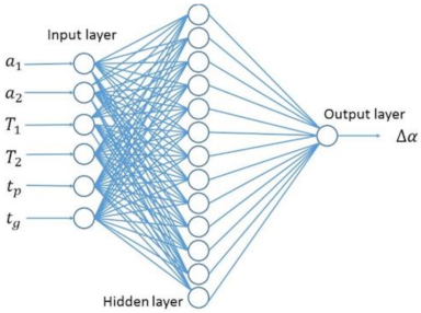
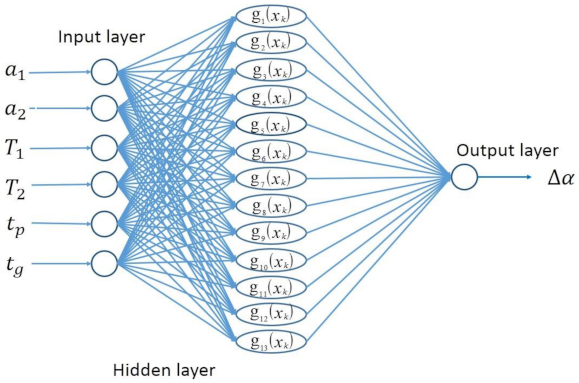
The network structure of the fully connected estimation model in this paper is shown in Figure 3.
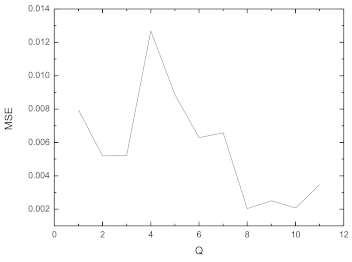
When designing the fully connected neural network according to the test, the number of network layers adopted a three-layer structure in which the input layer was one, the hidden layer was one and the output layer was one. This paper took six factors as the input and one factor as the output so the number of input layer nodes was six and the output layer node was one. The number of nodes in the hidden layer is usually determined by the Kolmogorov theorem [19]. In order to find the optimal number of hidden layer nodes, we selected the value near the optimal hidden layer node number obtained by Equation (5) for a trial calculation where Q was the number of nodes in the hidden layer and d was the number of nodes in the input layer in the Formula.
The result is shown in Figure 4. The MSE are the mean square errors of the 20 sets of test data.
Combining empirical formulas and trial calculations, it was found that when the number of hidden layer nodes of the fully connected neural network model was eight, the estimated training effect of the model could meet the training requirements better. In this paper, the transfer function was selected as the Sigmoid function, the learning rate was 0.003 and the training target was the mean square error MSE ≤ 0.002. When the mean square error met the requirements, the training ended. Using Python to write code to realize the training model, we found that after training 623 times, the MSE met the set error requirements and the operation took 0.374 s.
3.3. DNN
3.3.1. Deep Neural Network
A DNN can be understood as a neural network with many hidden layers. Empirically, a greater depth does seem to result in better generalization for a wide variety of tasks. This suggests that using deep architectures does indeed express a useful priority over the space of functions that the model learns [20].
3.3.2. The Establishment of a DNN
The number of network layers of the neural network described in Section 3.1 adopted a three-layer structure in which the hidden layer was one. In order to enhance the expressive ability of the model, the hidden layer of the DNN neural network estimation model became two. As there were many combinations of double-layer hidden layers and we discovered that the mean square error of the models was not much different from each other after a trial calculation, we decided to choose the same number of nodes in the two hidden layers. Considering the total training time, the optimal number of hidden layer nodes of the DNN was nine and the remaining parameters were the same as the previous fully connected neural network estimation model.
3.4. RBF Neural Network
The RBF neural network was a three-layer neural network, which also included an input layer, a hidden layer and an output layer. The transformation from input space to hidden layer space was nonlinear while the transformation from hidden layer space to output layer space was linear. The basic idea of implementing an RBF neural network was to use the RBF as the “base” of the hidden unit to form a hidden layer space. The basis function in the hidden layer locally responded to the input signal and transformed the low-dimensional pattern data into the high-dimensional space, making the hidden layer nodes produce a larger output so that linearly inseparable problems in the low-dimensional space could be linearly separable in the high-dimensional space. The RBF neural network could approximate any nonlinear function and had a good generalization ability. The activation function used a radial basis function:
where was the input vector, was the basis function center, was the radius of the RBF kernel function, n was the number of samples and c was the number of hidden layer nodes.
The relationship between the input and output of the RBF neural network was:
where indicated the connection weight of the hidden layer nodes. The remaining parameters were the same as the fully connected neural network model above. The network structure of the RBF estimation model in this paper is shown in Figure 5.
For the RBF neural network regression model of autoclave forming in this paper, the model training effect could be optimized by modifying the number of hidden layer nodes and the radius of the kernel function, . We used the GridSearchCV function of the “Scikit-Learn” package in Python to perform a grid search to find the optimal parameters for the model. After the calculation, the best parameter combination of the RBF neural network regression model in this paper was that Q = 21, = 0.4 and the mean square error was 0.000115 at that time.
3.5. SVR Model
A support vector machine (SVM) is a class of generalized linear classifiers that perform binary classifications on data by supervised learning. The basic principle of the SVM is to follow the inner product function. SVR (support vector regression) is an important application branch in the SVM. The difference between the SVR and the SVM classification was that there was only one type of sample point in the SVR, which sought the optimal hyperplane to minimize the total deviation of all sample points from the hyperplane. The SVR transformed the input space into a high-dimensional feature space through a nonlinear transformation defined by an inner product kernel function and returned in the high-dimensional feature space, which was as follows:
where was the feature space, w was the weight and b was the bias. According to the principle of structural risk minimization, the weight coefficient w and the deviation b could be minimized to obtain the following objective function [21]:
where was loss function. In order to minimize the Euler norm and also to control the fitting error beyond precision, the relaxation variables and were introduced where one was the number of samples. The optimization problem in Equation (9) could then be transformed into a constraint minimization problem, namely:
where C was the penalty coefficient. To derive the dual problem of the original problem in Equation (10), the Lagrange multiplier was introduced to establish the Lagrange equation of the original problem. We then found the partial derivative of the Lagrange function separately (the partial derivative value was zero). Substituting the result into the Lagrange equation, the dual problem of the original problem could be obtained:
In this way, the original problem became a convex quadratic programming problem. By solving this quadratic programming problem, we obtained the model of the support vector regression machine:
where was the kernel function, was the input vector, was the sample vector that was already known and was the radius of the RBF kernel function.
For the autoclave forming SVR model in this paper, the model training effect could be optimized by modifying the penalty coefficient C and the kernel function radius . We used the GridSearchCV function of the “Scikit-Learn” package in Python to perform a grid search to find the optimal parameters for the model. After the calculation, we found that the optimal parameter combination of the SVR model in this paper was C = 200 and = 0.2. At that time, the MSE was 0.005769.
3.6. KNN Regression Model
The idea of KNN (K-Nearest Neighbor) is that if most of the K most similar samples in a feature space (that is, the nearest neighbors in a feature space) belong to a certain category, then the sample also belongs to this category. The principle of the KNN regression model in this paper was the same as the KNN classification problem. For the input vector , we picked k samples that were nearest and regarded the average of their as the predicted value in order to find the corresponding value on the regression curve. For the distance between the sample data and the data to be predicted, we used the Euclidean distance:
where indicated the sample vector that was already known and n indicated the number of input nodes.
For the KNN regression model of autoclave forming in this paper, the K value could be modified to make the model training effect the best. We used the GridSearchCV function of the “Scikit-Learn” package (Scikit-Learn, 0.14, open-source, France) in Python to perform a grid search to find the optimal parameters for the model. After the calculation, we found that the optimal parameter combination of the KNN regression model in this paper was K = 1. At that time, the MSE was 0.000122.
4. Results and Discussion
By comparing the MSE of the five prediction models, as shown in Table 4, the accuracy of these five prediction models could be judged.
It can be seen from Table 4 that the MSE of the RBF prediction model was the smallest and its prediction effect was the best; the KNN, DNN, RBF prediction models were not much different from each other in the MSE and they were in the same order of magnitude. In general, the MSE of the five prediction models were all less than 0.006, which could complete the prediction task accurately. We then took the remaining five sets of verification data in the sample shown in Table 5 and used the trained model to predict it and normalize the results. The results are shown in Table 6.
In order to make the results more intuitive, the absolute errors of the five prediction models are listed in Table 7 and the relative errors of the five prediction models are listed in Table 8:
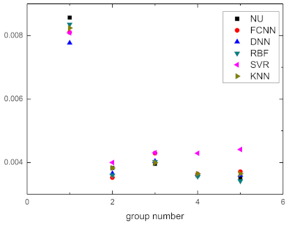
It could be seen that when the five prediction models predicted the difference of the maximum curing degree of the verification set, except for the large error of the SVR model, the rest were within −10% to 10%, which was consistent with the test results. In order to make the observation intuitive, all of the predicted and actual values of the verification sets are depicted in Figure 6. The NU in Figure 6 is the numerical value. As shown in Figure 6, the predicted value of the SVR was generally far away from the actual value. However, these five sets of data were simply to verify the prediction effect of the model. There might have been a few errors between the different sets of data that could be reduced by obtaining more sets of verification data. The five sets of data could not reflect the overall accuracy so we estimated the accuracy of the models according to the MES. The calculation with ABAQUS took about 1200 s each time, while it only took a few seconds for the machine learning model to complete the calculation after the five kinds of machine learning models were trained with the appropriate amount of original data. For a new set of input values, using a trained machine learning prediction model could greatly save computing time. The value predicted by machine learning could meet the actual needs to guide production. However, the quality of the model was not only reflected in the model error. In many cases, we considered additional requirements: the smoothness of the model, the ability to handle noise, the uncertainty estimation and so on. In the future, we will continue other research to improve the evaluation of the model. This technology is of great significance for engineering practice because the composite parts with a good curing degree have good properties.
Stefaniak et al. [22] proposed that due to the uneven curing of composite laminates and the existence of the stress gradient, the residual stress will be generated after curing, resulting in the deformation of composite laminates. The uniformity of the curing degree could be obtained in a short time, which could quickly identify whether the selected process parameters could produce good quality composite parts.
5. Conclusions
- The models based on machine learning for the prediction of the uniformity of the degree of cure of the composite in an autoclave had a small error margin and high efficiency, greatly saving manpower and time. These models provided a new and effective method for the estimation of the maximum ∆α of a composite in autoclave forming.
- Based on the estimated maximum curing degree difference, we could quickly find the curing process parameter group with the smaller maximum ∆α so as to reduce the residual stress in the composite molded parts and provide convenience for the optimization of the composite molding process.
- In the five machine learning prediction models including a fully connected (FC) neural network model, a deep neural network (DNN) model, a radial basis function (RBF) neural network model, a support vector regression (SVR) model and a K-nearest neighbors (KNN) model, the prediction effect of the RBF neural network model was the best, the prediction effect of the SVR model was the worst and the prediction effects of the KNN model and the DNN model were better when predicting the maximum ∆α.
- Compared with the experimental test method, the machine learning prediction models had the advantages of low cost and high speed but the method had certain errors. If sufficient data cannot be provided, the calculation result will be inconsistent with the true value. The accuracy of the result also depends on the training data. Compared with a numerical simulation, this method also had the advantages of low cost and high speed but this method could only obtain the final numerical results and could not dynamically reflect the reaction process. Therefore, the specific method to be used must be analyzed in conjunction with the actual situation.
- In future work, in order to improve the accuracy of the prediction model, an ensemble learning of five machine learning models will be constructed to obtain excellent generalization performance. the integration method may be boosting, bagging or random forest.
Author Contributions
Writing—original draft, Y.L.; writing—review and editing, Z.G. All authors have read and agreed to the published version of the manuscript.
Funding
This research received no external funding.
Institutional Review Board Statement
Not applicable.
Informed Consent Statement
Not applicable.
Data Availability Statement
Not applicable.
Acknowledgments
Thanks for the assistance by Ren Chao (Department of electronics and communication engineering, Shanghai Jiao Tong University, Shanghai, 200240, China) and his intelligent wife Jin Dengchao.
Conflicts of Interest
The authors declare no conflict of interest.
References
- Loos, A.C.; Springer, G.S. Curing of Epoxy Matrix Composites. J. Compos. Mater. 1983, 17, 135–169. [Google Scholar] [CrossRef] [Green Version]
- Hojjati, M.; Hoa, S. Curing simulation of thick thermosetting composites. Compos. Manuf. 1994, 5, 159–169. [Google Scholar] [CrossRef]
- Johnston, A.A. An integrated model of the development of process-induced deformation in autoclave processing of composite structures. Ph.D. Thesis, The University of British Columbia, Ann Arbor, MI, Canada, July 1998. [Google Scholar]
- Hoa, S.V. Design and manufacturing of composites. In An Investigation of Autoclave Convective Heat Transfer, 2nd ed.; Johnston, A., Hubert, P., Vaziri, R., Poursartip, A., Eds.; Technomic Pub.: Lancaster, PA, USA, 1998. [Google Scholar]
- Dolkun, D.; Zhu, W.D.; Xu, Q.; Yinglin, K.E. Optimization of cure profile for thick composite parts based on finite element analysis and genetic algorithm. J. Compos. Mater. 2018, 52, 155–181. [Google Scholar] [CrossRef]
- Blest, D.C.; Duffy, B.R.; McKee, S.; Zulkifle, A.K. Curing simulation of thermoset composites. Compos. Part A 1999, 30, 1289–1309. [Google Scholar] [CrossRef]
- Khan, A.; Kim, N.; Shin, J.K. Damage assessment of smart composite structures via machine learning: A review. JMST Adv. 2019, 1, 107–124. [Google Scholar] [CrossRef] [Green Version]
- Cheung, A.; Yu, Y.; Pochiraju, K. Three-dimensional finite element simulation of curing of polymer composites. Finite Elem. Anal. Des. 2004, 40, 895–912. [Google Scholar] [CrossRef]
- Kim, Y.K.; White, S.R. VISCOELASTIC ANALYSIS OF PROCESSING-INDUCED RESIDUAL STRESSES IN THICK COMPOSITE LAMINATES. Mech. Adv. Mater. Struct. 1997, 4, 361–387. [Google Scholar] [CrossRef]
- Kempner, E.A.; Hahn, H.T.; Huh, H. The effect of the aged materials on the autoclave cure of thick composites. In Proceedings of the International Conference of Composite Materials/11, Gold Coast, QLD, Australia, 14–18 July 1997; pp. 422–431. [Google Scholar]
- Gao, T.L. Simulation and Control Methods of Curing Deformation of Thermosetting Resin Matrix Composites; Northwestern Polytechnical University: Xi’an, China, 2018. [Google Scholar]
- Liu, X.T. Study on Data Normalization in BP Neural Network. Mech. Eng. Autom. 2010, 6, 122–126. [Google Scholar]
- Jiao, L.C. Theory of Neural Network System; Xidian University Press: Xi’an, China, 1990. [Google Scholar]
- WU, J.T.; Wang, J.H. Neural Network Technology and Its Application; Harbin Engineering University Press: Harbin, China, 1998. [Google Scholar]
- Zhang, D.F.; Ding, W.X.; Lei, X.P. Matlab Programming and Comprehensive Application; Tsinghua University Press: Beijing, China, 2012; pp. 1–3. [Google Scholar]
- Lin, S.G.; Ou, Y.X. Research of the Optimization of the Learning Parameters in BP Neural Network; Microcomputer Information: Guangzhou, China, 2010. [Google Scholar] [CrossRef]
- Hecht-Nielsen, R. Theory of the Backpropagation Neural Network—Based on “nonindent”. In Proceedings of the International Joint Conference on Neural Networks, Hoffman Estates, IL, USA, 18–22 June 1989; Harry Wechsler. Elsevier: Amsterdam, The Netherlands, 1992; pp. 65–93. [Google Scholar]
- Jiang, J.X.; Wang, B.; Wang, M.; Cai, S.G.; Ni, T.; Ao, Y.F.; Liu, Y. Study on Natural Lighting Design for CDUT Library Based on BIM and BP Neural Network. J. Inf. Technol. Civ. Eng. Archit. 2020, 12, 30–38. [Google Scholar] [CrossRef]
- Robert, H.N. Kolmogorov’s Mapping Neural Network Existence Theorem. In Proceedings of the International Conference on Neural Networks, San Diego, CA, USA, 21–24 June 1987; Volume 3, pp. 11–13. [Google Scholar]
- Ian, G.; Yoshua, B.; Aaron, C. Deep Learning: Adaptive Computation and Machine Learning Series; MIT Press: Cambridge, MA, USA, 2016. [Google Scholar]
- Smola, A.J.; Schölkopf, B. A tutorial on support vector regression. Stat. Comput. 2004, 14, 199–222. [Google Scholar] [CrossRef] [Green Version]
- Stefaniak, D.; Kappel, E.; Spröwitz, T.; Hühne, C. Experimental identification of process parameters inducing warpage of autoclave-processed CFRP parts. Compos. Part A Appl. Sci. Manuf. 2012, 43, 1081–1091. [Google Scholar] [CrossRef]
Figure 1.
Typical cure profile.

Figure 2.
Schematic diagram of the simulation results.

Figure 3.
Structure of a fully connected network model.

Figure 4.
The results of trials to establish the optimum architecture of the FCNN.

Figure 5.
The structure of the RBF network model.

Figure 6.
Actual values of the verification set.


Table 1.
Thermal properties and cure kinetic constants for AS4/3501-6 composites.
| 1578 | 1578 | 0.4135 | 12.83 | 198.6 × 10³ | |
| 2.102 × 10⁹ | 2.014 × 10⁹ | 1.960 × 10⁵ | 8.07 × 10⁴ | 7.78 × 10⁴ | 5.66 × 10⁴ |
is the density of the composites; is the specific heat; and are the transverse and longitudinal thermal conductivities of the composite; is the ultimate heat of reaction; is the frequency factor; is the activation energies.
Table 2.
Range of process parameters.
| Range | [1, 5] | [1, 5] | [115, 155] | [175, 215] | [0, 100] | [0, 150] |
Table 3.
Curing data.
| Δα | ||||||
|---|---|---|---|---|---|---|
| 4 | 2 | 135 | 212 | 133 | 15 | 0.013438 |
| 3 | 1 | 134 | 198 | 5 | 98 | 0.006745 |
| 3 | 4 | 135 | 212 | 129 | 15 | 0.010842 |
| 4 | 2 | 127 | 204 | 133 | 14 | 0.018056 |
| 3 | 3 | 120 | 180 | 120 | 60 | 0.007668 |
| 3 | 1 | 115 | 194 | 122 | 24 | 0.00391 |
| 4 | 3 | 147 | 199 | 22 | 82 | 0.00553 |
| 1 | 3 | 146 | 198 | 84 | 10 | 0.011303 |
| 1 | 4 | 141 | 190 | 87 | 46 | 0.007735 |
| 5 | 2 | 116 | 201 | 8 | 35 | 0.00844 |
and are the two heating rates; and are the two holding times; and are the two holding temperatures.
Table 4.
The MSE of the five prediction models.
| Models | FCNN | DNN | RBF | SVR | KNN |
|---|---|---|---|---|---|
| MSE | 0.00203 | 0.000722 | 0.000115 | 0.005769 | 0.000122 |
Table 5.
Five sets of verification data.
| Group | Actual Value | ||||||
|---|---|---|---|---|---|---|---|
| 1 | 3 | 3 | 120 | 181 | 120 | 60 | 0.008564 |
| 2 | 2 | 1 | 119 | 178 | 120 | 60 | 0.003828 |
| 3 | 1 | 1 | 119 | 178 | 120 | 60 | 0.003957 |
| 4 | 1 | 1 | 117 | 177 | 111 | 66 | 0.003597 |
| 5 | 1 | 1 | 116 | 176 | 105 | 70 | 0.003512 |
Table 6.
Actual value and predicted value.
| Group | Actual Value | FC Predicted Value | DNN Predicted Value | RBF Predicted Value | SVR Predicted Value | KNN Predicted Value |
|---|---|---|---|---|---|---|
| 1 | 0.008564 | 0.007715 | 0.007767 | 0.008355 | 0.008082 | 0.008237 |
| 2 | 0.003828 | 0.003707 | 0.003657 | 0.003602 | 0.004 | 0.003828 |
| 3 | 0.003957 | 0.004324 | 0.004044 | 0.004027 | 0.004311 | 0.003995 |
| 4 | 0.003597 | 0.003797 | 0.003625 | 0.003561 | 0.004291 | 0.003645 |
| 5 | 0.003512 | 0.003823 | 0.003609 | 0.003417 | 0.00441 | 0.003645 |
Table 7.
The absolute errors of the five prediction models.
| Group | FC | DNN | RBF | SVR | KNN |
|---|---|---|---|---|---|
| 1 | −0.00031 | −0.0008 | −0.00021 | −0.00048 | −0.00033 |
| 2 | −0.00051 | −0.00017 | −0.00023 | 0.000171 | 2.49 × 10⁻¹¹ |
| 3 | −2.7 × 10⁻⁵ | 8.68 × 10⁻⁵ | 6.97 × 10⁻⁵ | 0.000354 | 3.8 × 10⁻⁵ |
| 4 | −0.00017 | 2.82 × 10⁻⁵ | −3.6 × 10⁻⁵ | 0.000693 | 4.73 × 10⁻⁵ |
| 5 | −3.7 × 10⁻⁵ | 9.68 × 10⁻⁵ | −9.5 × 10⁻⁵ | 0.000898 | 0.000132 |
Table 8.
The relative errors of the five prediction models.
| Group | FC | DNN | RBF | SVR | KNN |
|---|---|---|---|---|---|
| 1 | −0.03655 | −0.09301 | −0.02434 | −0.05625 | −0.03816 |
| 2 | −0.13318 | −0.04485 | −0.05916 | 0.044781 | 6.51 × 10⁻⁹ |
| 3 | −0.00677 | 0.021937 | 0.017619 | 0.089503 | 0.009611 |
| 4 | −0.0465 | 0.007825 | −0.01004 | 0.192761 | 0.013157 |
| 5 | −0.01056 | 0.027568 | −0.02696 | 0.255647 | 0.037712 |
Publisher’s Note: MDPI stays neutral with regard to jurisdictional claims in published maps and institutional affiliations. |
© 2021 by the authors. Licensee MDPI, Basel, Switzerland. This article is an open access article distributed under the terms and conditions of the Creative Commons Attribution (CC BY) license (https://creativecommons.org/licenses/by/4.0/).
Share and Cite
MDPI and ACS Style
Lin, Y.; Guan, Z. The Use of Machine Learning for the Prediction of the Uniformity of the Degree of Cure of a Composite in an Autoclave. Aerospace 2021, 8, 130. https://0-doi-org.brum.beds.ac.uk/10.3390/aerospace8050130
AMA Style
Lin Y, Guan Z. The Use of Machine Learning for the Prediction of the Uniformity of the Degree of Cure of a Composite in an Autoclave. Aerospace. 2021; 8(5):130. https://0-doi-org.brum.beds.ac.uk/10.3390/aerospace8050130
Chicago/Turabian StyleLin, Yuan, and Zhidong Guan. 2021. "The Use of Machine Learning for the Prediction of the Uniformity of the Degree of Cure of a Composite in an Autoclave" Aerospace 8, no. 5: 130. https://0-doi-org.brum.beds.ac.uk/10.3390/aerospace8050130
Note that from the first issue of 2016, this journal uses article numbers instead of page numbers. See further details here.