Numerical Aspects of Particle-in-Cell Simulations for Plasma-Motion Modeling of Electric Thrusters

Abstract

The present work is focused on a detailed description of an in-house, particle-in-cell code developed by the authors, whose main aim is to perform highly accurate plasma simulations on an off-the-shelf computing platform in a relatively short computational time, despite the large number of macro-particles employed in the computation. A smart strategy to set up the code is proposed, and in particular, the parallel calculation in GPU is explored as a possible solution for the reduction in computing time. An application on a Hall-effect thruster is shown to validate the PIC numerical model and to highlight the strengths of introducing highly accurate schemes for the electric field interpolation and the macroparticle trajectory integration in the time. A further application on a helicon double-layer thruster is presented, in which the particle-in-cell (PIC) code is used as a fast tool to analyze the performance of these specific electric motors.

1. Introduction

Electric thrusters have aroused much interest in space applications in recent years [1]. The most attractive characteristic of this kind of propulsion is the capability to deliver a very high specific impulse [2,3] and potentially long service life [4,5]. These features are essential for many futuristic, but not far, missions, as well as the building of a near-Earth satellite infrastructures, or the colonization of the Moon and Mars [6,7,8]. Hall-effect thrusters are the most developed propulsion system for satellites, and they are currently in use in a number of telecommunication and government spacecrafts [9]. Their power spans from 100 W to 20 kW, with thrust between a few mN and 1 N, and specific impulse values between 1000 s and 3000 s. On the other hand, other kinds of technology are preferred in low power applications [10] as Cubesat thrusters, in which the available power is limited by the surface of the solar panels exposed to the Sun. In this case, the propulsion system is mainly used for precise attitude control in formation flight and this includes: microcathode arc thrusters that use electrical arcs to convert solids into plasma; electrospray systems that generate microdroplets or ions; thrusters based on field emissions that produce energetic ions [11]. The plasma propulsion is also important for the precise positioning of the satellites with scientific instruments [12]. An example is the LISA Pathfinder mission for gravitational wave detection for which the spacecraft uses colloid thrusters for drag-free control [13], or the counterpart of that program, i.e., the Chinese Taiji satellite constellation program whose success depends on the pointing performance of the equipped electric thrusters [14].

Following the large interest in electric thrusters, different types of numerical schemes have been developed, beginning with exploiting one-dimensional models along the axial direction inside the channel in the late 1990s, until developing, in the subsequent years, an extension to the near-field region where the magnetic field is still large [15,16]. Overall, there are three main computational approaches used for plasma exhausts [17]: fluid models, in which the electrons and the ions are treated as fluids [18,19,20]; kinetic models, in which both species are described by the employment of macroparticles [21,22]; hybrid models, in which the electrons are dealt with as a fluid, while the ions as a group of macroparticles [23,24].

Hybrid models are the best compromise for computational cost and physics description. In this kind of model, the ions are described by particle-in-cell (PIC), while particular treatments are adopted for electrons. Two kinds of PIC codes can be recognized depending on the kind of equations used for the electric potential computation: the electromagnetic one, which uses the full set of Maxwell’s equations, including both plasma source terms (charge density and plasma currents) and external source terms (e.g., a polarized electrode), and the electrostatic one, in which the problem is simplified, and Maxwell’s equations are replaced by the Poisson’s equation.

In space electric thruster applications, the former is suitable to describe the internal flow-field of high-power thrusters as Hall-effect thrusters [25,26], while the latter for cathodeless thrusters [27,28,29]. The accuracy of the solution is mostly affected by the implemented numerical scheme and by the number of macroparticles involved in the simulation. Reaching high accuracy is important for the estimation of the ion exit velocity, which affects the evaluation of the thrust and the specific impulse. On the other hand, time dependent physical phenomena as plasma instabilities can be captured only by an accurate simulation of the plasma motion. In fact, the correct estimation of the plasma frequency is essential to identify the kind of instability. For example, ionization instability is typically characterized by low frequency oscillations ranging from 10–30 kHz [30], while gradient-drift instabilities are a result of high frequency oscillations in 1–10 MHz [31]. For these reasons, a sophisticated numerical approach which, in turn, implies a significant computational effort, is required.

The main hybrid approaches for plasma thrusters have been recently reviewed by Taccogna et al. [15]. The most common literature approach appears to be the following: firstly, the electric field is computed in each node by using a simple finite difference method; then, the ion trajectory integration is performed by a leapfrog method with a bi-linear interpolation of the electric field on the particle position for the computation of the ion acceleration. Most of the reviewed approaches do not take into account the details of the mass conservation during the ionization process, nor of an appropriate boundary reflection. All of them deal with sequential processing, thereby discarding the possibilities offered by modern, off-the-shelf computing platforms.

Setting up a reliable numerical scheme for the dealt with problem is cumbersome and the usual strategy of exploiting a high-level programming language, such as Matlab, to ease the debugging process increases the computational time, and therefore the calculation can be hardly accomplished in a reasonable duration. Graphics processing units (GPUs) have been established in the last years as off-the-shelf, massively parallel computing platforms, usable for high-performance scientific computing [32,33]. Thanks to CUDA (Compute Unified Device Architecture) [34], significant speedups have been observed for several computational problems. Most recently, high-level languages, such as Matlab, have acquired the capability of running portions of code accelerated by GPU processing [35]. The accelerating code can be written directly in CUDA and compiled in a linkable source for the highest performance or in Matlab-like instructions for ease of use with some cost in performance. This is very useful to accelerate the most computationally burdened portions of the numerical scheme by the GPU, while appointing the CPU to act as an easy-to-use coding front-end.

In this paper, we propose a highly accurate scheme for the calculation of the macroparticle motion having the following features:

• Fourth order Runge–Kutta integration scheme, instead of the typically used leapfrog integration;
• Cubic bi-spline interpolation [32] of the electric potential, instead of the typically used bi-linear interpolation;
• A new ray-tracing approach to reflect the particles at the domain boundaries; note that a full description of the algorithm used for the treatment of the boundary walls is generally not provided throughout the literature approaches;
• A new neutrals ionization scheme;
• Use of parallel programming on GPU.

The approach has the following advantages:

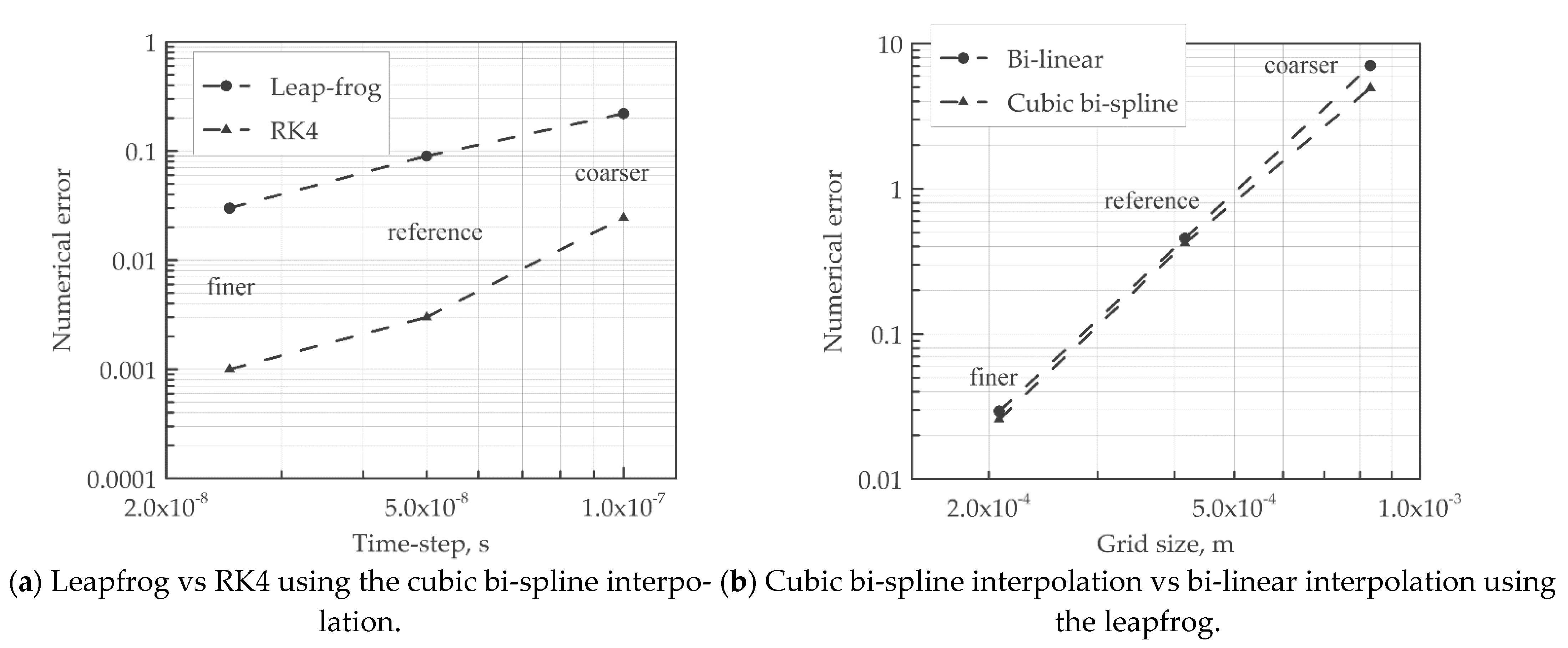
• The Runge–Kutta scheme significantly improves the accuracy over the leapfrog scheme;
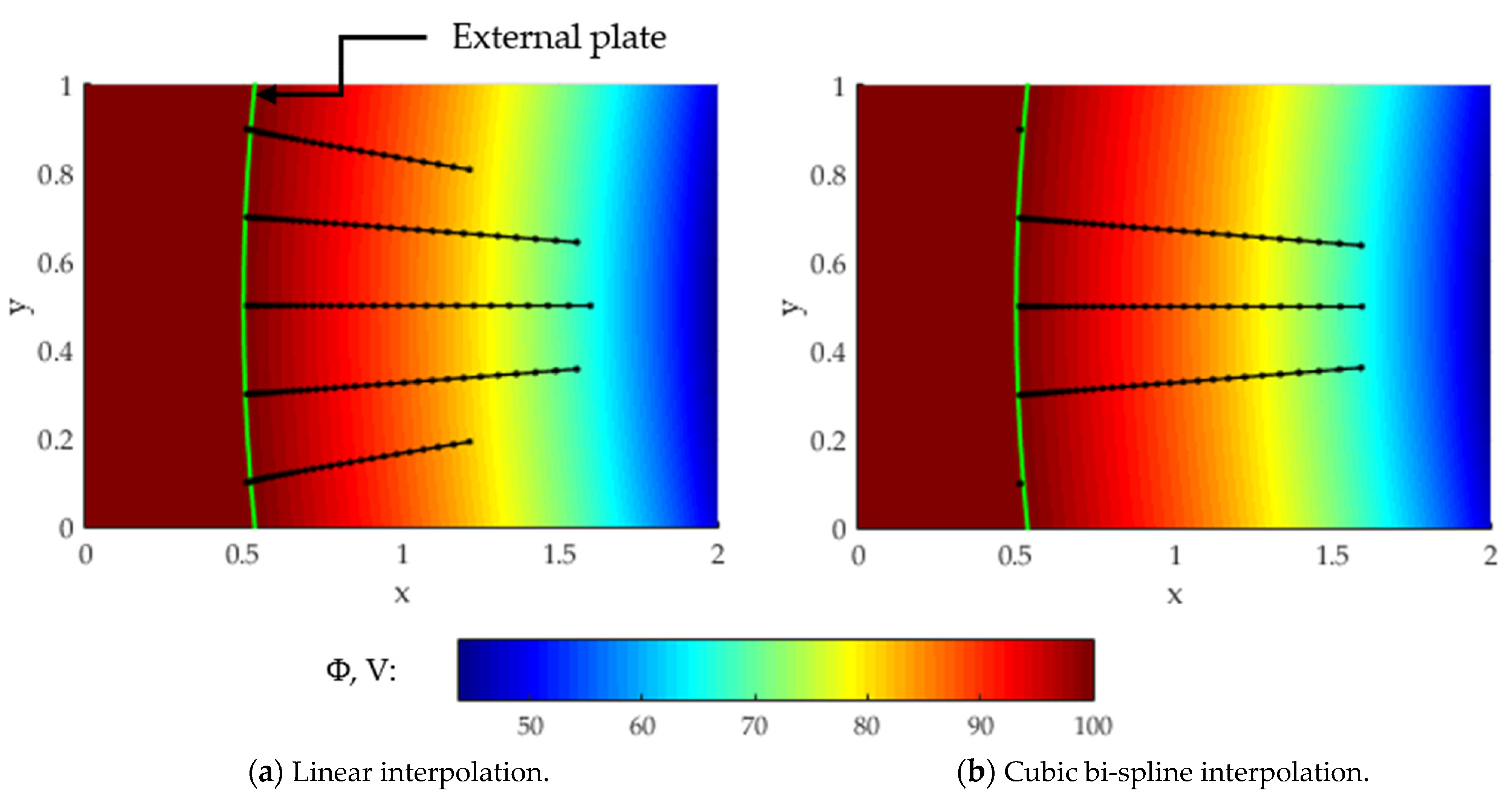
• The cubic bi-spline interpolation improves the accuracy over bi-linear interpolation, ensures the continuity of the first derivative and consequently of the electric field, and enables analytical differentiation once determined the interpolation coefficients;
• The ray-tracing scheme enables us to reflect on the particles quickly;
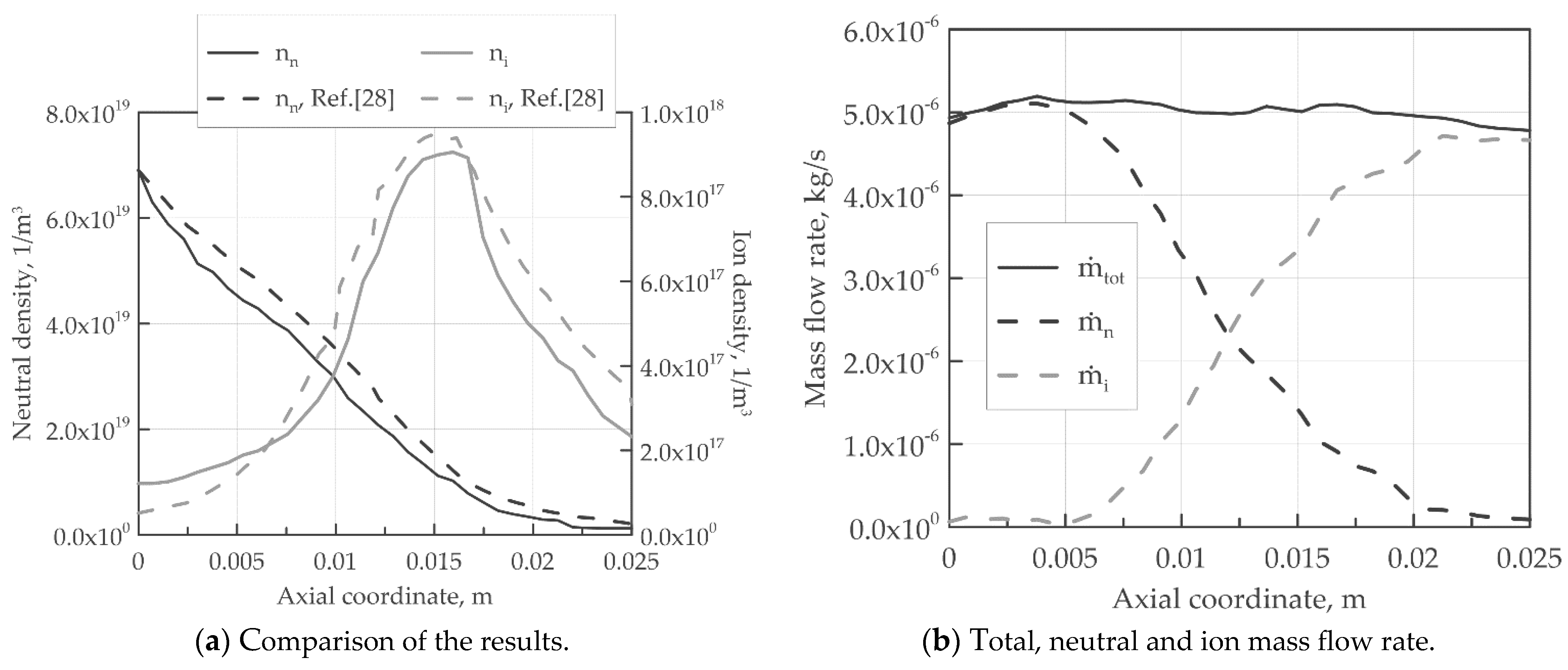
• The neutrals ionization scheme fully conserves the total mass flow rate;
• GPU processing enables us to manage the increased computational burden associated to the accuracy improvements, to reach convenient computation time on off-the-shelf computing platforms.

We would like to emphasize that the advancements shown in this paper do not concern a better knowledge of the plasma physics, but rather an improvement of tools already available in the literature, which are essential to avoid erroneous theoretical insights.

In this paper, the PIC approach is implemented in MatLab, and its most demanding parts accelerated in CUDA. To solve the problem, extremely accurate numerical schemes are introduced and compared with the typical literature solutions. The code has been validated on previous numerical results, and two applications on the Hall-effect thrusters and on the helicon double-layer thrusters have been reported. In particular, a bidimensional geometry has been considered in the first case, while a one-dimensional version has been employed in the second case.

The paper is organized as follows. Section 2 is devoted to describing a complete in-house bidimensional PIC model, in which high accurate schemes to integrate the ion macroparticle trajectories and to interpolate the electric field on the ion positions are introduced. The approaches used for the treatment of the boundary walls and the neutral ionization are detailed, and an innovative computational strategy to save computational time is presented. In Section 3, a one-dimensional version of the PIC code is applied to the case of a helicon double-layer thruster coupled with a non-linear Poisson’s solver for the computation of the electric potential. In Section 4, the results of the presented numerical model are shown. Firstly, an application on a Hall-effect thruster is used to validate the overall numerical model. The benefits gained by the highly accurate schemes and the computational strategy employed are shown. Finally, the results obtained by the model used to compute the performance of a helicon double-layer thruster are displayed.

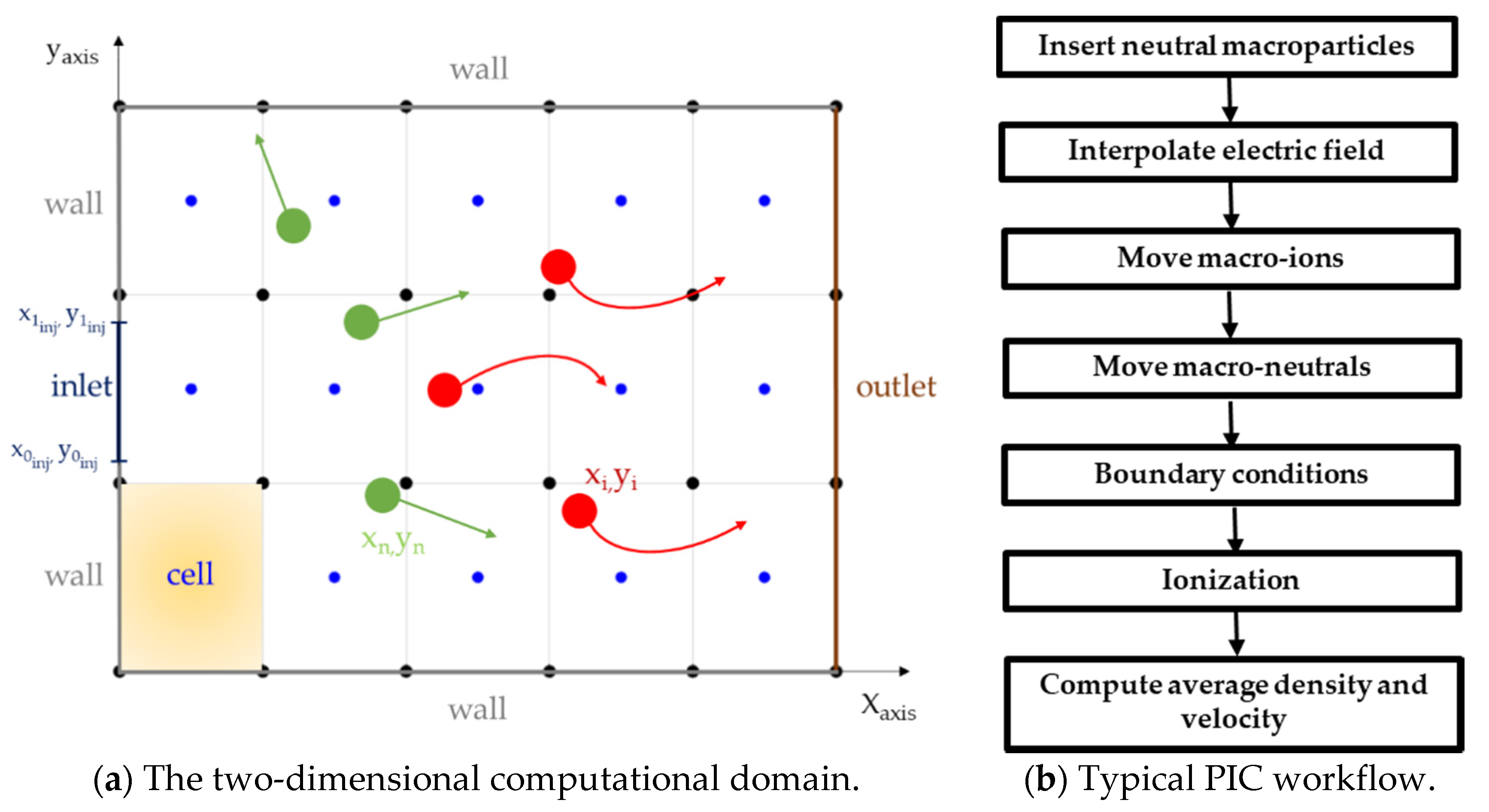
2. PIC Numerical Apparatus

In this section, the two-dimensional PIC approach used for modelling the plasma motion inside the Hall-effect thruster is described. An analogous one-dimensional algorithm has been developed following the same guidelines in order to obtain a useful tool to predict the performance of a helicon double-layer thruster in Section 3.

In the two-dimensional case, the numerical domain is assumed rectangular and consists of a Cartesian grid composed of nodes and cells, as can be seen in Figure 1a. The electric potential, which is needed for the computation of the electric field for the motion of the ions, is defined at the nodes, and it is assumed to be constant in time, when considering the Hall-effect thruster. Opposing this, the potential will be computed, time after time, by solving a non-linear Poisson equation in the helicon double-layer thruster. Average quantities, as mass density and velocity, are defined and assumed constants in the cells.

The plasma consists of a mixture of ions and electrons, whose masses are significantly different. For this reason, as well known, the electrons are modelled as a fluid, while the ions are a discrete number of particles, and are tracked during the time. Since the computational cost of the PIC method is strictly linked to the number of particles involved in the simulation, the particles are clustered as “macroparticles”, which represent groups of ions or neutrals characterized by the same mass, position, and velocity.

Three kinds of boundaries are available in the code: injection inlet, along which the neutral macroparticles, are inserted in the domain; wall boundaries, along which the macroparticles, are reflected; and outlet, across which the macroparticles are eliminated.

The physical time has been linearly discretized with a suitably low time step, $∆t$ [36]. In this work, in both the considered cases, the electron temperature is assumed to be known; hence, the modelling of the electronic fluid is not required. Concerning the motion of the macroparticles, the neutrals move according to a rectilinear uniform motion, while ions accelerate for the presence of the electric field. Because the node space coordinates could not coincide with the ion positions, an interpolating tool was set up, which can compute the electric field in any position of the ion macroparticle within the interior of the computational domain.

When the ions and neutrals impact the domain boundaries, they are reflected diffusively back to the computational domain by a fast ray-tracing algorithm, described in Section 2.2.

Finally, the ionization process is described in Section 2.4. In particular, different from other approaches available in the literature [26], the method developed in this work fully preserves the conservation of the total mass flow rate.

In this Section, the physical equations and the numerical apparatus are described in detail, in order to allow an easy implementation for the reader. Figure 1b shows a general PIC scheme, each block of which is described in-depth below. We will begin with the description of the neutral and ion macroparticle motion, which represents the core of the solution strategy.

2.1. Neutral and Ion Macro-Particles Motion

The equations of the motion for neutral and ion macroparticles are:

$$\begin{gathered} \frac{d{\mathit{u}}_{\mathit{i}}}{dt}={\mathit{a}}_i=\frac{q_i}{m_i}{\mathit{E}}_{\mathit{i}} \\ \frac{d{\mathit{x}}_{\mathit{i}.\mathit{n}}}{dt}={\mathit{u}}_{\mathit{i},\mathit{n}} \end{gathered}$$

(1)

where ${\mathit{x}}_{\mathit{i}.\mathit{n}}$, ${\mathit{u}}_{\mathit{i},\mathit{n}}$ and ${\mathit{a}}_{\mathit{i}}$ are the particle position, velocity, and acceleration vectors; ${\mathit{E}}_{\mathit{i}}$ is the vector of the interpolated electric field and $q_i/m_i$ is the mass to charge ratio, which is the same for all macroparticles. Bold quantities represent vectors including axial (x-axis) and radial (y-axis) components, and the subscripts i and n indicate that the quantity is associated with the ion or neutral macroparticle, respectively. Equation (1) points out that the neutral’s velocity remains constant along the trajectory, as mentioned at the beginning of the Section.

The accuracy of the numerical model strongly depends on the type of the temporal integration scheme and on the type of the electric field interpolation on the particle position. The integration of Equation (1) is usually performed by a leapfrog scheme which has second-order accuracy [36], and the ion acceleration is obtained by a linear interpolation of the local electric field on the particle position, which has first-order accuracy. In this work, an effort has been made to introduce highly accurate schemes, in particular, a Runge–Kutta scheme (RK4) with fourth order accuracy for the integration in time and a cubic bi-spline interpolation [32] with third order accuracy for the interpolation of the electric potential and the consequent computation of the electric field on the particle position. Concerning the calculation of the electric field, we notice that it depends not only on the adopted interpolation scheme, but also on the way the electric potential is differentiated. The numerical differentiation is usually performed by a second order central difference method. As will be further stressed later, the use of the cubic bi-spline interpolation will enable us to perform such a differentiation analytically. The use of highly accurate schemes has increased the number of mathematical operations, which can be performed in a reasonable time, only involving parallel programming, the strategy of which is described in the next sections. The quantities to be integrated into Equation (1) are evaluated at the next temporal timestep, $t_{k+1}$, from the current position ${\mathit{x}}_{\mathit{k}}$ at the present timestep, $t_k$, plus the weighted average of four increments:

$$\begin{gathered} {\mathit{x}}_{\mathit{k}+\mathbf{1}}={\mathit{x}}_{\mathit{k}}+\frac{1}{6}{\left(\mathbf{∆}\mathit{x}\right)}_0+\frac{1}{3}{\left(\mathbf{∆}\mathit{x}\right)}_1+\frac{1}{3}{\left(\mathbf{∆}\mathit{x}\right)}_2+\frac{1}{6}{\left(\mathbf{∆}\mathit{x}\right)}_3 \\ {\mathit{u}}_{\mathit{k}+\mathbf{1}}={\mathit{u}}_{\mathit{k}}+\frac{1}{6}{\left(\mathbf{∆}\mathit{u}\right)}_0+\frac{1}{3}{\left(\mathbf{∆}\mathit{u}\right)}_1+\frac{1}{3}{\left(\mathbf{∆}\mathit{u}\right)}_2+\frac{1}{6}{\left(\mathbf{∆}\mathit{u}\right)}_3 \end{gathered}$$

(2)

where ${\mathit{u}}_{\mathit{k}}$ is the axial and radial velocity components. The four increments for the particle position and position are evaluated as follows:

$$\begin{array}{cc}{\left(\mathbf{∆}\mathit{x}\right)}_{\mathbf{0}}={\mathit{u}}_{\mathit{k}}\mathbf{∆}t,& {\left(\mathbf{∆}\mathit{u}\right)}_{\mathbf{0}}={\mathit{a}}_{{\mathit{x}}_{\mathit{k}}}\mathbf{∆}t,\\ {\left(\mathbf{∆}\mathit{x}\right)}_{\mathbf{1}}=\left({\mathit{u}}_{\mathit{k}}+\frac{{\left(\mathbf{∆}\mathit{u}\right)}_0}{2}\right)\mathbf{∆}t,& {\left(\mathbf{∆}\mathit{u}\right)}_{\mathbf{1}}=\left({\mathit{a}}_{{\mathit{x}}_{\mathit{k}}}+{\mathit{a}}_{{\mathit{x}}_{\mathbf{1}}}\right)\mathbf{∆}t,\\ {\left(\mathbf{∆}\mathit{x}\right)}_{\mathbf{2}}=\left({\mathit{u}}_{\mathit{k}}+\frac{{\left(\mathbf{∆}\mathit{u}\right)}_{\mathbf{1}}}{2}\right)\mathbf{∆}t,& {\left(\mathbf{∆}\mathit{u}\right)}_{\mathbf{2}}=\left({\mathit{a}}_{{\mathit{x}}_{\mathit{k}}}+{\mathit{a}}_{{\mathit{x}}_{\mathbf{2}}}\right)\mathbf{∆}t,\\ {\left(\mathbf{∆}\mathit{x}\right)}_{\mathbf{3}}=\left({\mathit{u}}_{\mathit{k}}+{\left(\mathbf{∆}\mathit{u}\right)}_{\mathbf{2}}\right)\mathbf{∆}t,& {\left(\mathbf{∆}u\right)}_{\mathbf{3}}=\left({\mathit{a}}_{{\mathit{x}}_{\mathit{k}}}+{\mathit{a}}_{{\mathit{x}}_{\mathbf{3}}}\right)\mathbf{∆}t,\end{array}$$

(3)

The ${\mathit{a}}_{\mathit{x}}$ terms are computed as:

$$\begin{gathered} {\mathit{a}}_{{\mathit{x}}_{\mathit{k}}}=\frac{q_i}{m_i}{\mathit{E}}_{\mathit{x}}({\mathit{x}}_{\mathit{k}}), \\ {\mathit{a}}_{\mathit{x}}{}_{\mathbf{1}}=\frac{q_i}{m_i}{\mathit{E}}_{\mathit{x}}({\mathit{x}}_{\mathit{k}}+{\left(\mathbf{∆}\mathit{x}\right)}_{\mathbf{1}}), \\ {\mathit{a}}_{\mathit{x}}{}_{\mathbf{2}}=\frac{q_i}{m_i}{\mathit{E}}_{\mathit{x}}({\mathit{x}}_{\mathit{k}}+{\left(\mathbf{∆}\mathit{x}\right)}_{\mathbf{2}}), \\ {\mathit{a}}_{\mathit{x}}{}_{\mathbf{3}}=\frac{q_i}{m_i}{\mathit{E}}_{\mathit{x}}({\mathit{x}}_{\mathit{k}}+{\left(\mathbf{∆}\mathit{x}\right)}_{\mathbf{3}}), \end{gathered}$$

(4)

It should be noticed that the employment of the cubic bi-spline interpolation offers the following advantages:

• It provides an interpolating polynomial which ensures at least the continuity of the first derivative as requested by the need of performing a spatial derivative of the potential to obtain the electric field; in this way, a continuous electric field is ensured;
• Once the coefficients of the interpolating cubic bi-spline polynomial of the electric potential have been obtained, differentiation can be directly performed to obtain the electric field with a reduction in the numerical effort.

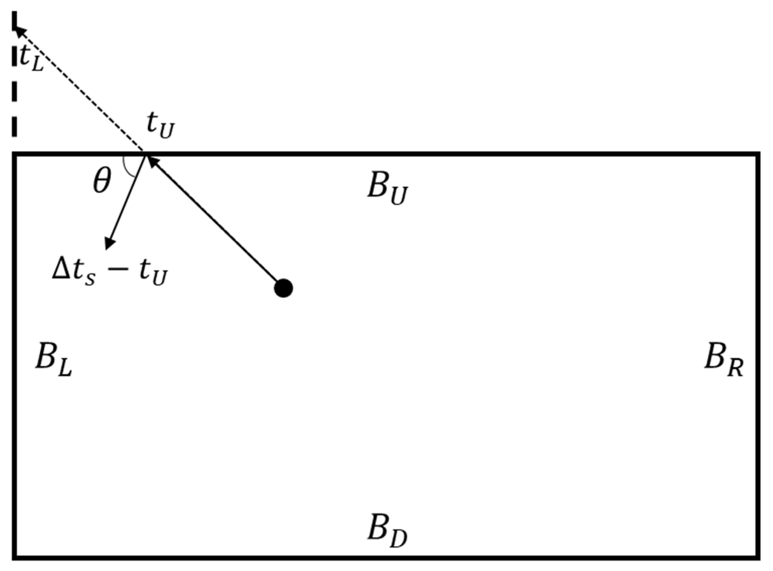
2.2. Boundary Conditions

The boundary conditions are employed when the macroparticle position is close to the boundary of the computational domain and is likely to exit it in the next time step. A ray-tracing approach has been devised to compute the particle position at the point of reflection. The strategy to compute the velocity at the reflection point is also illustrated below. The ray-tracing approach is valid for a generic shape of the domain boundaries and, of course, for the considered rectangular geometry.

The macroparticle position is checked at each of the four-time substeps considered by the RK4 scheme. If the particle exits the domain in any one of the substeps, then it is changed to neutral, and the substep $∆t_s$, at which the boundary has been crossed, is saved for computing the reflection. Then, ray tracing, consisting of the points below, takes place:

• The particles substep, giving rise to the boundary-crossing, is rewinded;
• The vector velocity at the rewinded substep is checked to determine the possible impact boundaries; for instance, as shown in Figure 2, negative axial and positive radial velocity components mean that only the upside or left-side boundaries $B_U$ and $B_L$ can have been crossed;
• The time to reach $B_U$ and $B_L$, $t_U$ and $t_L$, respectively, is evaluated, and the smallest one defines the crossed boundary;
• The particle is moved back to the computational domain for a physical time corresponding to the remaining part of the time substep after the impact time, which amounts to $∆{\mathrm{t}}_{\mathrm{s}}-t_U$ for the case illustrated in Figure 2; the movement velocity is computed according to the approach detailed below;
• The updated particle position is checked and, if it has crossed a domain boundary again, the ray-tracing algorithm is invoked once more;
• If an outlet boundary condition is enforced at the crossed boundary, the macroparticle is just eliminated.

The x- and y-components of the reflection speed are directly sampled from a 2D thermal Maxwellian distributions as described in [37]:

$$\begin{gathered} u=v_{mp}\sqrt{-\ln \left(R_1\right)}\cos \theta \\ v=v_{mp}\sqrt{-\ln \left(R_1\right)}\sin \theta \\ \theta =-\pi R_2 \end{gathered}$$

(5)

where the most probable speed, $v_{mp}$, is defined as $\sqrt{2k_b{T}_w/m_i}$, $R_1$ and $R_2$ are uniformly distributed random numbers ranging between 0 and 1, $T_w$ is the wall temperature, which is assumed constant, and $k_b$ is the Boltzmann constant. $\theta$ is the reflection angle of the impacting macroparticle, which spans a negative half-round corner for the upper wall, but it can be easily extended to the remaining walls.

2.3. Injection

A number of neutral macroparticles are placed each time step at the chamber inlet. The weight of each macroparticle depends on the enforced inlet mass flow rate. A high number of injected macroparticles at each time step increases the resolution of the flow field, and it improves the statistics in each cell. However, a large number of macroparticles could be prohibitive. We have nevertheless experienced that 20 macroparticles injected at each time step is a good compromise between solution accuracy and computational effort.

The macroparticle injection position ($x_p$, $y_p$) is randomly selected within the inlet region illustrated in Figure 1a. It is drawn by the following equation:

$$\begin{gathered} x_p=x_{0_{inj}}+R_3\left(x_{1_{inj}}-x_{0_{inj}}\right) \\ {y}_p=y_{0_{inj}}+R_3\left(y_{1_{inj}}-y_{0_{inj}}\right) \end{gathered}$$

(6)

where $R_3$ is a random number, uniformly distributed between 0 and 1 and $x_{0_{inj}}$, $x_{1_{inj}}$, $y_{0_{inj}}$ and $y_{1_{inj}}$ are the endpoints of the injector inlet, which reduces to a line in a two-dimensional frame, namely, $x_{0_{inj}}=x_{1_{inj}}$. Concerning the initial injection speed, a similar approach as for the boundary reflection has been adopted, assuming a most probable speed corresponding to the inlet temperature.

2.4. Ionization

Ionization takes place by electron impact on the neutrals. Direct Simulation Monte Carlo methods are not applicable to simulate ionization because the electrons are treated as a fluid. Standard Monte Carlo Collision methods are not applicable either, because neutral particles are the dominant species, the neutral flux is highly reduced along the chamber, and ion and neutral particles have very different masses [38]. In this paper, only a single charge ionization per volume unit is considered, which can be kinetically modelled as:

$$\dot{n_i}=\zeta \left(T_e\right)n_n{n}_i$$

(7)

where $n_n$ and $n_i$ are the neutral and the ion particle density, while $\zeta \left(T_e\right)$ is the Drawin ionization model. In Equation (7), the ion particle density appears in place of the electron particle density, having assumed quasi-neutrality of the fluid. Furthermore, $\zeta$ represents the number of collisions per unit time [39]. It should be noticed that, for fixed gas molecular properties, the ionization model is only a function of the electron temperature. The neutral and ion density of Equation (7) are computed in each cell by simply dividing the total mass of the particles placed in each cell for the corresponding volume. In this way, weighting functions have been dismissed [36]. A new approach has been developed in the present work to completely preserve the total mass in each cell, which is described by the following points:

• The estimation of the ionized mass, M_i, in each cell, is obtained by multiplying Equation (7) by Δt. If the estimation exceeds the total neutral mass of a cell, which is physically unfeasible, then the newly ionized cell mass is saturated to the corresponding neutral total mass;
• The newly ionized mass is divided by the number of neutral macroparticles in the corresponding cell to obtain an average mass to be subtracted to each neutral macroparticle. However, since the macroparticles can be characterized by different masses, the mass to be subtracted can be higher than the mass of a certain neutral macroparticle. In this case, to simplify, the remaining mass to be ionized is equally subtracted to the masses of the other neutral macroparticles placed in the same cell;
• New ion macroparticles are generated. Henceforth, we will assume that, at each time step, a constant number of 40 macroparticles are generated. For them, the ion macroparticle mass is computed by dividing the total ionized mass by the number of the generated macroparticles;
• The two velocity components of each ion macroparticle are evaluated by the same algorithm as illustrated in Section 2.2, in which $\theta$ spans now a full round corner and the local electron temperature is used for the estimation of $v_{mp}$.

2.5. Averages

At the end of the process, detailed in the previous Subsections, the updated macroparticle quantities, e.g., the velocity and the mass, are averaged on the cell. The density is computed as the ratio between the total macroparticles mass contained in a cell and the corresponding cell volume, while the cell velocity is computed by a mass-weighted average of the macroparticle velocities. In this way, weighting functions [36] are dismissed. The average quantities are used to compute the cell ionization rate, as mentioned in Section 2.4, and to obtain a continuous visualization of the quantities in the computational domain. In addition, continuous quantities from the PIC model could be required as inputs to integrate the electron equations when the electron fluid is modelled.

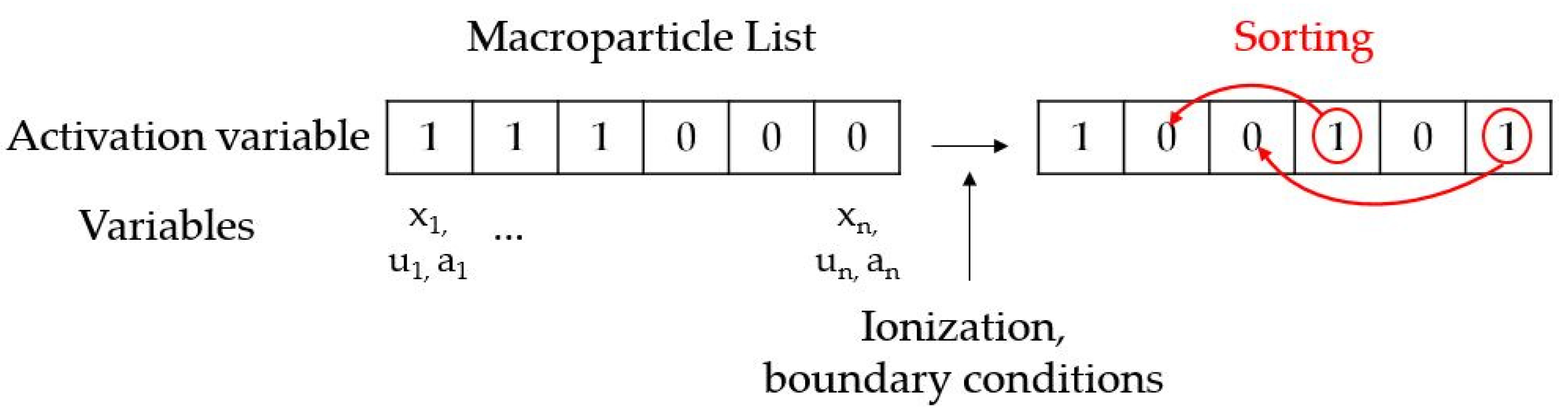
2.6. Computational Strategy

In this Subsection, the employed computational strategy is sketched. Notwithstanding the fairly basic structure of the motion equations, the number of mathematical computations involved by a large number of particles, typically around 100,000, is obviously large, and the related computational burden should be properly dealt with. Fortunately, the problem lends itself to a massively parallel treatment because, at each timestep, the macroparticles move independently along their own trajectory.

We note that, according to the recent review paper [16], the approach presented here is the very first one to exploit GPU computing for a PIC application in plasma thrusters. The parallelization illustrated in [16] has been carried out using the message passing interface (MPI) protocol which is radically different from the single instruction multiple data (SIMD) paradigm of GPUs, and which typically involves the use of large computational mainframes, while in this paper, we are targeting off-the-shelf computational platforms.

Prior to proceeding with parallelization, the approach has been entirely developed in MatLab language, both to enable a simple debug, and to obtain a reference for performance evaluation. A profiling of such a code has then been worked out, which has evidenced that the most time-consuming operations are those related to the interpolation stage. The embarrassing parallelism of most of the operations has thus enabled to parallelize most of the code in a simple way. A large part of the implementation has been performed by “high-level” programming, that is, by defining the quantities of interest on the GPU as GPUArrays and by exploiting the device-agnosticism of MatLab functions. According to the profiling results, only the electric field interpolating subroutine has been coded by using a CUDA __global__ function.

To indulge the massive parallelism, two independent lists of neutrals and ion macroparticles are generated at the beginning of the calculation: they are handled and updated during the simulation. These lists store all of the information about the macroparticles, such as position, velocity components, mass, etc. A logic variable is introduced in order to quickly identify whether the particle is operating or not. In particular, when the particle is injected, this variable is set to 1; for the particles which leave the domain from the outlet boundary or they are completely consumed during the ionization, the variable turns to 0. At the end of each timestep, these lists are sorted to cluster the active particles at the top. The total number of operating particles is also computed at each time step. In this way, the CUDA kernels can operate on the only active particles. This guarantees a massive parallelism by avoiding thread divergence due to branches or, even worse, the need to sift the active particles, which would unavoidably lead to uncoalesced memory accesses. The approach to keep the macroparticle (ions and neutrals) lists ordered is illustrated in Figure 3.

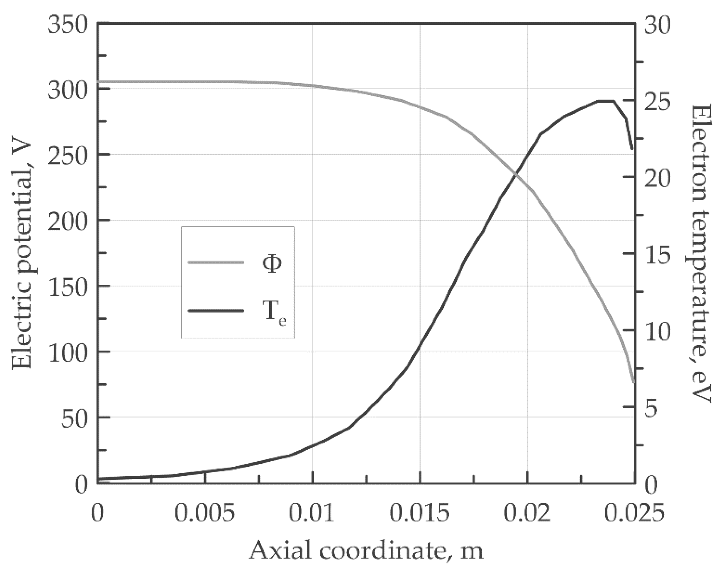
3. Helicon Double-Layer Thruster Modelling

In this section, the one-dimensional problem of modelling helicon double-layer thrusters is described. A quasi-1D version of the PIC model described in Section 2 has been coupled with a non-linear Poisson’s equation, explained below. The physical domain is shown in Figure 4a, and it represents the most external line of the magnetic field produced by the motor solenoids shown in [40,41]. The corresponding one-dimensional computational domain is shown in Figure 4b, and it consists of a linear series of nodes and cells. The thrust chamber range is between 0.3 and 0.6 m, while the external magnetic channel is placed between 0 and 0.3 m. For the sake of simplicity, ion macroparticles are directly spread into the chamber by a random algorithm similar to Equation (7). Hence, the ionization rate $SR$ (which is equal to ${\dot{n}}_i{V}_{ch}$) and the electron temperature are the inputs of the model. The ions crossing the right boundary are reflected by the ray-tracing algorithm, while those crossing the left boundary are removed.

As mentioned in Section 2, different from the Hall-effect thruster, the electric potential is not kept constant during the simulation and, accordingly, a non-linear Poisson solver is required to compute the electric potential field in each node of the one-dimensional domain. In fact, in these thrusters, the assumption of quasi-neutrality is no longer valid, and the Poisson equation is introduced:

$${\frac{\mathrm{d}\varphi }{\mathrm{dx}}}^2=-\frac{\rho }{{\epsilon }_0}$$

(8)

where ϕ is the electrostatic potential, ${\epsilon }_0$ is the vacuum permittivity, and $\rho$ is the charge density that can be written as the difference between the electron and ion density:

$$\rho =q\left(n_i-n_e\right)$$

(9)

Equation (8) becomes non-linear when the Boltzmann approximation is considered to hold true for the electrons. In particular, in order to derive the density of the Boltzmann electrons, the starting point is the electron momentum equation [42]:

$$m_e{n}_e{\dot{u}}_e=-n_{e}q\frac{\mathrm{d}\varphi }{\mathrm{dx}}-\frac{\mathrm{d}{p}_e}{\mathrm{dx}}$$

(10)

where m_e is the electron mass and p_e is the electron pressure. Under the Boltzmann approximation, the left-hand side of Equation (10) is assumed to be zero, so that Equation (10) becomes a balance of forces:

$$n_{e}q\frac{\mathrm{d}\varphi }{\mathrm{dx}}=-\frac{\mathrm{d}{p}_e}{\mathrm{dx}}$$

(11)

Assuming an isothermal electron fluid, the electron pressure can be written in terms of the electron temperature, resulting in:

$$n_{e}q\frac{\mathrm{d}\varphi }{\mathrm{dx}}=k_b{T}_e\frac{\mathrm{d}{n}_e}{\mathrm{dx}}$$

(12)

Equation (12) can be easily integrated obtaining the expression of the electron density:

$$n_e=n_0{e}^{\frac{q\varphi \left(x\right)}{k_b{T}_e}}$$

(13)

where n₀ is the Boltzmann density parameter which corresponds to the value of the electron density when the potential is enforced to be equal to zero. Equation (13) does not take into account the effects of the variation of the cross-sectional area of the fluid domain on the electron density. Following [43] for one-dimensional approaches, the density can be corrected as:

$$n_e\left(x\right)=n_e\frac{r_{ch}^2}{r^2\left(x\right)}$$

(14)

where $r_{ch}$ is the chamber radius and r is the duct radius at the generic axial coordinate x. Equation (14) is a generalization of Equation (13) for quasi-1D problems. Therefore, the non-linear Poisson equation can be rewritten as:

$$\frac{d^2\varphi }{d{x}^2}=\frac{q}{{\epsilon }_0}\left[n_0{e}^{\frac{q\varphi \left(x\right)}{k_b{T}_e}}\frac{r_{ch}^2}{r^2\left(x\right)}-n_i\right]$$

(15)

where $q$ is the electron charge. In order to solve Equation (15), two boundary conditions are needed, and for the case of interest, two Dirichlet boundary conditions have been chosen:

$$\varphi \left(x=0\right)=0, \varphi \left(x=L\right)=0$$

(16)

For the problem of interest, the ion density is computed following the application of a one-dimensional version of the PIC described above. The Boltzmann density parameter is computed from the electron particle number balance equation:

$$\frac{d{N}_e}{dt}={\dot{n}}_i-n_0{v}_e{A}_{exit}$$

(17)

where $N_e$ is the number of electrons in the domain, $A_{exit}$ is the exit cross-sectional area of the magnetic duct, and $v_e$ is the electron thermal velocity defined as $\sqrt{e{T}_e/\left(8\pi m_e\right)}$. Enforcing the time derivative of Equation (17) equal to zero (steady-state assumption), the Boltzmann density parameter can be obtained as:

$$n_0=\frac{{\dot{n}}_i}{v_e{A}_{exit}}$$

(18)

Deriving a solution to Equation (16) requires a dedicated numerical scheme to address the non-linearity involved by the exponential of the electric potential [44,45]. Once the electric potential in each node has been computed, the ion particles are moved by the PIC algorithm; then, the electric potential is updated, and the loop is repeated until the steady-state condition is reached, namely, when the variation of the thrust and of the specific impulse fall below a prefixed tolerance value.

4. Results and Discussion

In this section, the results obtained by the new numerical model described above are illustrated. Concerning the two-dimensional case, firstly, the PIC model was validated on the results reported in [37], in particular, by benchmarking against the described experimental test on the SPT-100 electric thruster [46]. Secondly, the advantages achieved by the implementation of the highly accurate numerical schemes are highlighted with respect to the typical methods employed in PIC technology and the computational time saved by coding for GPU computations is shown. Finally, the results of the one-dimensional version of the PIC code are presented to demonstrate the capability of the numerical model to perform a fast analysis to predict the helicon double-layer thruster performance.

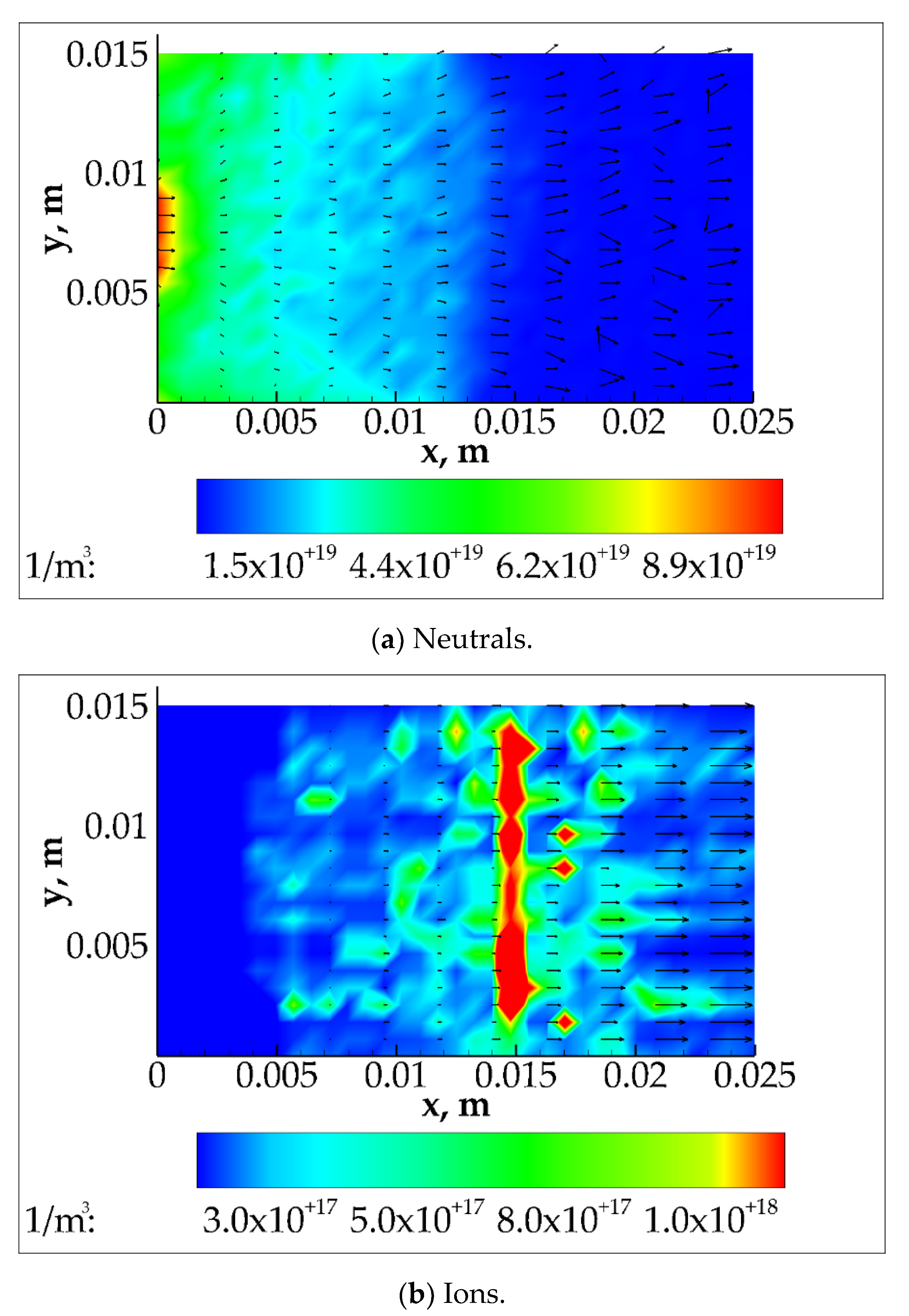
4.1. Application to a Hall-Effect Thruster and Code Validation

In this Subsection, the validation of the new two-dimensional PIC model described above is carried out on a numerical test case concerning a Hall-effect thruster application and the results are compared with those shown in [37], obtained by an usual PIC method. In order to set up a test case to compare with the literature results, the mesh grid and the temporal timestep are taken in the same way as the reference work. An analysis on the spatial/temporal mesh size will be a matter for future work. The two-dimensional domain is a box of 0.025 × 0.015 m discretized by 34 × 22 nodes, and it represents the accelerating channel of the thruster shown in the reference work. The modelling of the outer channel flow field is avoided. The simulation time is set to 5 × 10⁻⁴ s with a time step of 5 × 10⁻⁸ s. The inlet neutral mass flow rate is fixed to be equal to 5 × 10⁻⁶ kg/s, and 20 neutral macroparticles are injected at each timestep. A temperature of 850 K is enforced at the walls and of 750 K at the inlet boundary. The typical execution time of our most optimized PIC code is around 56 min. The electron temperature and electric potential used in the simulation are shown in Figure 5.

Figure 6 shows the neutrals and plasma density contours with the velocity vectors. A highly neutral density region is placed in the proximity of the anode where the neutrals are injected, which decreases along the axial coordinate due to the ionization process of the neutrals. A recirculation zone is detected in the proximity of the upper-left and bottom-left corners. On the other hand, the ion density peak takes place in correspondence with the region in which the product $\zeta \left(T_e\right)·n_n$ reaches its maximum. After the peak, the velocity increases exponentially, due to the electric potential drop near the channel exit, and consequently, the density drops down in order to conserve the total particles’ number. To compare the results obtained in the present work with that shown in the reference work, the one-dimensional distribution of neutral and ion densities is shown in Figure 7a. The plots are obtained averaging the distribution along the radial coordinate. A good agreement between the numerical results is displayed. Finally, Figure 7b shows the total, the neutral, and the ionized mass flow rate computed along the axial coordinate and, as stated above, the total mass flow rate is fully conserved.

4.2. Accuracy Assessment

With the aim of highlighting the benefits gained by the new methods employed in this PIC model (which are RK4) and the bi-cubic spline interpolation, the performance of the proposed approach is compared with that of the most popular schemes for the targeted applications, which are the leapfrog and the bilinear interpolation. The integration schemes are compared when the same interpolation scheme is adopted; later on, the integration scheme is fixed, and the interpolation techniques are compared.

A single particle was placed in the domain at 0 m along the axial coordinate and 0.0075 m along the radial coordinate, with an initial axial velocity of 150 m/s and zero radial velocity. Since the motion along the radial coordinate is negligible, the analysis involves only nodes placed along the x-axis. The numerical domain, the mesh grid and the electric potential were kept the same as that in Figure 6.

Table 1. Axial grid step and timesteps.

	Δx	Δt
Time integration		2.5 × 10−8 s
	4.16 × 10−4 m	5 × 10−8 s
		1 × 10−7 s
Space interpolation	8.3 × 10−4 m
	4.16 × 10−4 m	5 × 10−8 s
	2.08 × 10−4 m

resumes the timestep and the grid-step employed in each parametric study. Referring to the RK4 versus leapfrog, coarser and finer temporal discretization was defined around a reference timestep of 5 × 10⁻⁸ s. The cubic bi-spline interpolation was used in both cases. On the other hand, when comparing bilinear and the cubic bi-spline interpolation, a coarser and finer spatial mesh was considered, based on a reference mesh with Δx equal to 4.16 × 10⁻⁴ m.

Figure 8a shows a log-log plot of the numerical error versus the time discretization, in which the final macroparticle velocity is the observed quantity, since the evaluation of the exit velocity affects the estimation of the motor specific impulse. The numerical error is the deviation of the computed value from the reference value calculated by Richardson’s extrapolation technique [47]. It appears that the RK4 scheme increases the accuracy against the leapfrog scheme. The numerical error drastically drops from 2.45 × 10⁻² to 1.9 × 10⁻³ in the RK4 method, while it decreases from 1.64 × 10⁻¹ to 6.31× 10⁻² for the linear interpolation.

Concerning the interpolation method, Figure 8b shows a log-log plot of the numerical error versus the spatial grid size for the final positions calculated with the cubic bi-spline and bilinear interpolations. Due to the small difference in accuracy between the two methods, the advantage of adopting the former emerges when dealing with highly non-linear and discontinuous electric potential fields. To prove the last statement, a test case with five particles moving in a discontinuous non-linear electric field generated via a capacitor with two circular and concentric thin plates is carried out. The considered domain is a 2 × 1 m box discretized by 100 × 50 nodes. The analytical electric potential [48] is obtained by assuming that the external plate is an iso-potential surface at 100 V with a radius of 3.5 m, while the internal is a likewise iso-potential surface at 0 V with a radius of 1.5 m. Both the surfaces are concentric with respect to a center placed at (2, 0) m. The test is performed by placing the five ion macro-particles equally spaced in the radial direction at a fixed axial coordinate of 0.5 m. As displayed in Figure 9, when using the linear interpolation method, the particles outside the capacitor are accelerated from left to right, despite the fact that they should not be influenced by the internal electric potential field. On the other hand, the bi-cubic spline interpolation fixes this issue, increasing the solution accuracy.

4.3. Computational Performance Enhancement via Parallelisation

In this Subsection, an analysis of the computational performance of the numerical code is carried out. Three versions of the new PIC model are presented in this work:

• The first version is completely executed sequentially, and all of the macro-particle operations are handled by using for loops;
• The second version is CPU multi-core accelerated and performs the operations for all the macroparticles in multi-core aware commands;
• The third version is accelerated on GPU.

The test case shown in Section 4.1 was run three times with the three different versions of the PIC code.

Table 2. Execution time comparison between the 3 different versions of the PIC code.

	CPU Parallel, Min	GPU Parallel, Min	Computational Gain, %
Execution time	101.2	55.75	44.91
RK4	43.65	23.18	46.89
Cubic bi-spline interpolation	40.22	19.80	50.77
Neutrals motion	7.31	3.45	52.80

summarizes the execution times of the second and third code versions with the corresponding computational gains, which are defined as the percentage of the saved time of the second version with respect to the time spent by the first version; the fully sequential code was totally unfeasible since it required 1.5 h to perform a single timestep. Despite the fact that the electron fluid is not modelled in the present work, the GPU parallel code execution time of 56 min appears to be better than that declared by Parra et al. [26] with an execution time of 200 min, and by Fife [36] with a time of 480 min, which are similar to that proposed in [37]. The execution time decreases drastically from the CPU parallel version to the GPU parallel version with a computational gain of 44.91%. Table 2 also displays the three most time-consuming routines that took the largest time of the total execution time. As expected, the slowest routines are the time integration, the electric field interpolation and the neutrals’ motion. Consequently, the computational cost of the macroneutrals is negligible, compared to that of the macroions (RK4 routine), whose number actually determines the total effort of a simulation. For all of the most time-consuming routines, the speedup achieved by parallelization, namely, the ratio between the sequential and parallel computational times, is around 2. As a consequence, the overall code has benefitted of an overall speedup of 2.

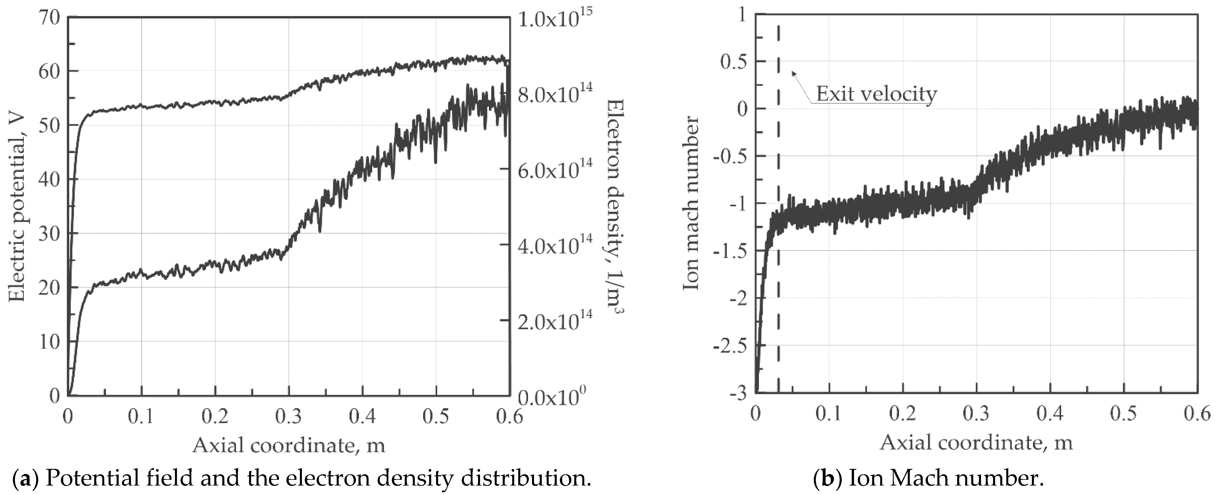
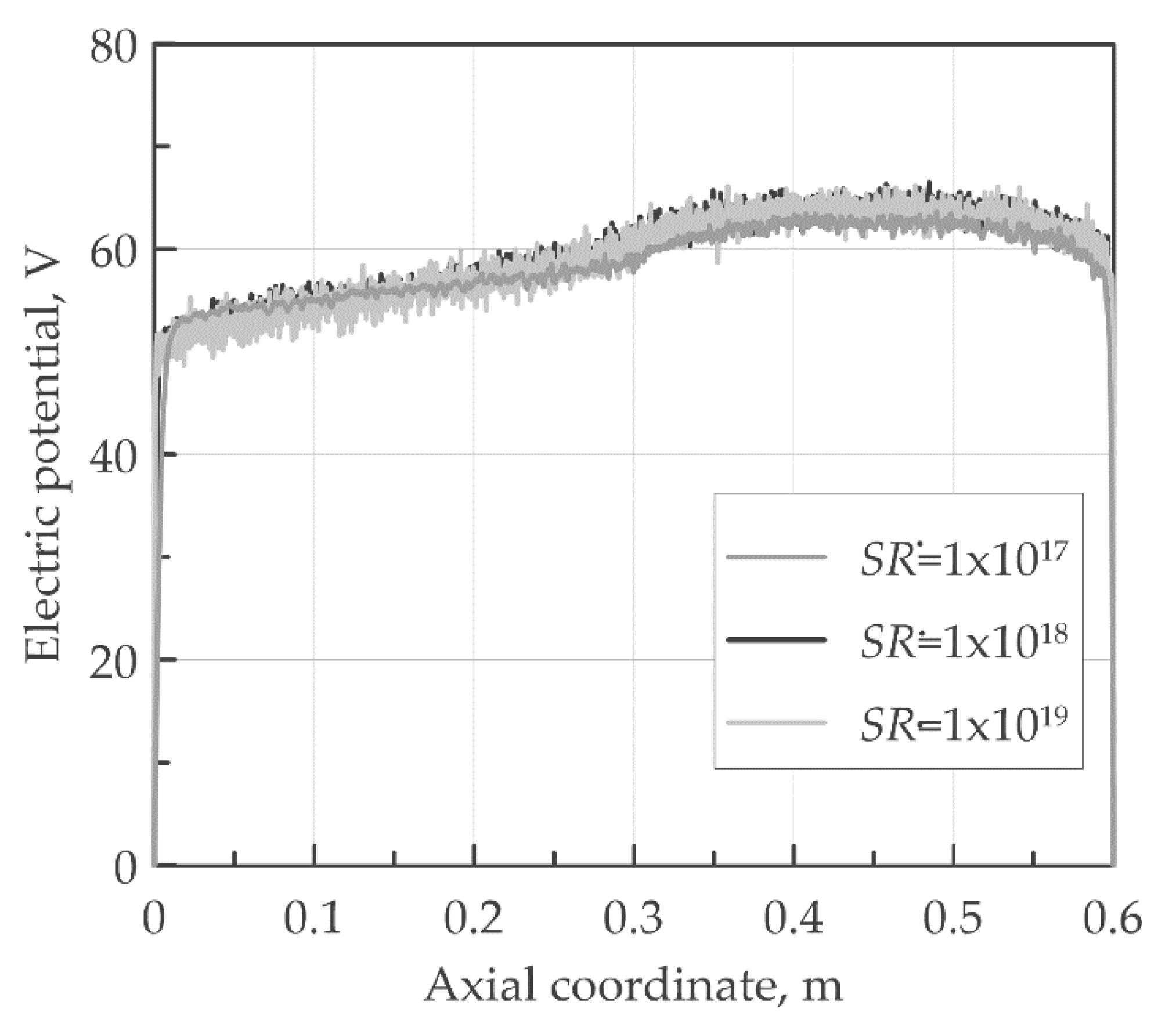
4.4. Magnetic Nozzle Thruster Application

In this Subsection, the results obtained by modelling a helicon double-layer thruster are shown. The computational domain is discretized by 2000 nodes. Figure 10 illustrates the results of the model when setting an electron temperature of 10 eV and 3 × 10¹⁶ particles per second of ionized argon. In the authors’ experience, five macroparticles are injected into the chamber at each timestep (1 × 10⁻⁷ s), which is a good arrangement to obtain a satisfactory numerical accuracy, and the steady-state is reached at around 1 × 10⁻³ s. The simulation involves around 150,000 macroparticles, and it lasts around 10 min. Figure 10a shows the potential drop of 12 V, which is mostly confined close to the chamber exit. Accordingly, the electron density increases exponentially with the electric potential approaching the maximum near the motor head. Figure 10b displays that the ions velocity is close to zero near the right wall and weakly supersonic in the external magnetic channel. It is worth pointing out that the velocity is negative, since the ions move from right to left. The specific impulse coincides with the ion exit velocity divided by the gravitational acceleration at the axial coordinate represented in the same picture. In this case, it is equal to 662 s, which well approximates the theoretical formula $Isp=v_i/g$, where the ion exit velocity is expressed as $\sqrt{2q∆\Phi /m_i}$. The thrust is obtained by multiplying the ion mass flow rate by the velocity at the same axial station, which is equal to 0.0126 mN.

A parametric study is performed to investigate the effect of increasing the electron temperature, keeping the ionization rate constant at a value of 1 × 10¹⁸. As shown in Figure 11a, the space-averaged potential increases with the electron temperature because the difference between the average ion and electron density is increasing. Indeed, observing Equation (18) the Boltzmann parameter is inversely proportional to the electron velocity. Hence, an increasing electron temperature implies an increasing electron velocity; accordingly, the Boltzmann parameter (and, consequently, the average electron density for Equation (13) decreases, involving a higher difference between the ion and electron distribution. A less obvious effect of the electron temperature on the thruster performance is shown in the same picture. A rise of the potential drop is experienced by changing the electron temperature with a consequent increment of the ion exit velocity. The resulting specific impulse is compared in Figure 11b with the theoretical formula, which appears to be featured by the same trend with the potential drop. To summarize, as expected, an augmentation of the fluid thermal energy improves the motor performance. Since the ion mass flow rate is kept constant, the thrust linearly increases with the specific impulse.

On the other hand, further simulations have been carried out varying the ionization rate and keeping the electron temperature constant at 10 eV. No significant effects have been observed on the electric potential, as shown in Figure 12. Accordingly, the potential drop and specific impulse remain approximately constant. Obviously, the thrust linearly increases with the ionization rate.

Finally,

Table 3. Comparison between the thrust performance by using argon and iodine gas at 10 eV, enforcing an ion mass flow rate of 6.5 × 10⁻⁸ kg/s.

Gas	Molecolar Weight, g/mol	Ionization Rate, Part/s	Potential Drop, V	Specific Impulse, s	Thrust, mN
Argon	39.95	1 × 1018	12.5	698	0.45
Iodine	126.90	3 × 1017	12.5	352	0.22

shows the difference in terms of performance employing argon or iodine ions assuming the electron temperature of 10 eV and the same ion mass flow rate of 6.5 × 10⁻⁸ kg/s. Consequently, an ionization rate of 1 × 10¹⁸ is enforced for the argon gas, while 3 × 10¹⁷ for the iodine gas, which is characterized by a molecular weight four times higher than argon. As shown, by enforcing the same ion mass flow rate, the best performance is obtained when considering the lighter gas, which confirms the capability of the numerical model to predict the performance for different gas properties.

5. Conclusions

A fast and accurate in-house particle-in-cell code has been presented in this work, which is able to reproduce the internal flow field of a Hall-effect thruster and to obtain fast performance analysis of a helicon double-layer thruster. Extremely accurate schemes have been introduced to integrate the macroparticle motion equations and to interpolate the electric field for computing the ions acceleration. The full two-dimensional PIC code has been validated on numerical literature results for the case of a Hall-effect thruster. The code has demonstrated to be able to reproduce the essential features of the internal flow field of a Hall-effect thruster. The accuracy has been compared with that achievable by methods usually employed in the literature. It has been proven that the employment of fourth order Runge–Kutta integration significantly improves the quality of the solution compared to the leapfrog method, when strong accelerations are involved in the flow field. On the other hand, despite the fact that the cubic bi-spline interpolation seems to achieve a similar accuracy compared to the bilinear, it is able to fix unphysical accelerations when the electric field is discontinuous. A computational strategy for reducing the computational time by using the GPU parallel computation is also proposed in this work. It has been demonstrated that the GPU computation allows for obtaining a significant computational gain of 44.91% with respect to other sequential or multi-core CPU options.

A series of parametric studies were performed in order to understand the effect of the input parameters on the helicon double-layer thruster performance. Firstly, the electron temperature was varied from 5 to 20 eV with a fixed ionization rate of 1 × 10¹⁸. The results show that the potential drop increases from 6 to 23 V, and accordingly, the specific impulse increases from 460 to 977 s. Then, no effects on the potential drop and on the specific impulse were found by changing only the ionizations rate. Finally, the kind of gas was switched from argon to iodine. The results show that the employment of a heavier gas deteriorates the motor performance, which in the case of iodine is around 50% than the argon.

Future developments of the present work may include:

• The extension of the geometry to non-rectangular domains; in this case, a Cartesian discretization would not be enough to describe the variations of the electric potentials at the domain boundaries and other kind of meshes, for example, a triangular mesh, should be employed;
• The extension of the geometry to 3D; for rectangular boundaries, the extension would amount to adding additional equations to account for third components of the fields; for non-rectangular boundaries, similarly to the point above, tetrahedral meshes should be employed;

It should be noticed that the proposed ray-tracing approach could be easily extended to general geometries and boundaries by referring to tangential planes. Another point of interest for future improvements of the approach regards obtaining a more realistic description of the plasma flow-field. Apart from modelling the electron fluid, which changes according to the kind of electric thruster, more faithful descriptions are required, including the plasma plume, the secondary electron emission, and the collisional models in the current PIC model. For all of the extensions, including the geometry and the accurate modelling, we expect that the improvements made by GPU computing will be even more relevant to make the approach run on off-the-shelf computing platforms.

References

1. Levchenko, I.; Xu, S.; Mazouffre, S.; Lev, D.; Pedrini, D.; Goebel, D.; Garrigues, L.; Taccogna, F.; Bazaka, K. Perspectives, frontiers, and new horizons for plasma-based space electric propulsion. Phys. Plasmas 2020, 27, 020601. [Google Scholar] [CrossRef] [Green Version]
2. Conde, L.; Domenech-Garret, J.L.; Donoso, J.M.; Damba, J.; Tierno, S.P.; Alamillo-Gamboa, E.; Castillo, M.A. Supersonic plasma beams with controlled speed generated by the alternative low power hybrid ion engine (ALPHIE) for space propulsion. Phys. Plasmas 2017, 24, 123514. [Google Scholar] [CrossRef]
3. Ding, Y.; Su, H.; Li, P.; Wei, L.; Li, H.; Peng, W.; Xu, Y.; Sun, H.; Yu, D.; Yongjie, D.; et al. Study of the catastrophic discharge phenomenon in a Hall thruster. Phys. Lett. A 2017, 381, 3482–3486. [Google Scholar] [CrossRef]
4. Voyager 1 Fires Up Thrusters after 37 Years. Available online: https://www.nasa.gov/feature/jpl/voyager-1-fires-up-thrusters-after-37 (accessed on 1 December 2017).
5. Croes, V.; Tavant, A.; Lucken, R.; Martorelli, R.; LaFleur, T.; Bourdon, A.; Chabert, P. The effect of alternative propellants on the electron drift instability in Hall-effect thrusters: Insight from 2D particle-in-cell simulations. Phys. Plasmas 2018, 25, 063522. [Google Scholar] [CrossRef]
6. Musk, E. Making Humans a Multi-Planetary Species. New Space 2017, 5, 46–61. [Google Scholar] [CrossRef]
7. Do, S.; Owens, A.; Ho, K.; Schreiner, S.; de Weck, O. An independent assessment of the technical feasibility of the Mars One mission plan—Updated analysis. Acta Astronaut. 2016, 120, 192–228. [Google Scholar] [CrossRef] [Green Version]
8. Levchenko, I.; Xu, S.; Mazouffre, S.; Keidar, M.; Bazaka, K. Mars Colonization: Beyond Getting There. Glob. Chall. 2019, 3, 1800062. [Google Scholar] [CrossRef] [PubMed] [Green Version]
9. Boeuf, J.-P. Tutorial: Physics and modeling of Hall thrusters. J. Appl. Phys. 2017, 121, 011101. [Google Scholar] [CrossRef]
10. Tummala, A.R.; Dutta, A. An Overview of Cube-Satellite Propulsion Technologies and Trends. Aerospace 2017, 4, 58. [Google Scholar] [CrossRef] [Green Version]
11. Levchenko, I.; Keidar, M.; Cantrell, J.; Wu, Y.-L.; Kuninaka, H.; Bazaka, K.; Xu, S. Explore space using swarms of tiny satellites. Nat. Cell Biol. 2018, 562, 185–187. [Google Scholar] [CrossRef] [Green Version]
12. Mazouffre, S. Electric propulsion for satellites and spacecraft: Established technologies and novel approaches. Plasma Sources Sci. Technol. 2016, 25, 033002. [Google Scholar] [CrossRef]
13. Armano, M.; Audley, H.; Auger, G.; Baird, J.; Binetruy, P.; Born, M.; Bortoluzzi, D.; Brandt, N.; Bursi, A.; Caleno, M.; et al. The LISA Pathfinder Mission. J. Phys. Conf. Ser. 2015, 610, 012005. [Google Scholar] [CrossRef] [Green Version]
14. Levchenko, I.; Xu, S.; Wu, Y.-L.; Bazaka, K. Hopes and concerns for astronomy of satellite constellations. Nat. Astron. 2020, 4, 1012–1014. [Google Scholar] [CrossRef]
15. Taccogna, F.; Garrigues, L. Latest progress in Hall thrusters plasma modelling. Rev. Mod. Plasma Phys. 2019, 3, 12. [Google Scholar] [CrossRef]
16. Kahnfeld, D.; Duras, J.; Matthias, P.; Kemnitz, S.; Arlinghaus, P.; Bandelow, G.; Matyash, K.; Koch, N.; Schneider, R. Numerical modeling of high efficiency multistage plasma thrusters for space applications. Rev. Mod. Plasma Phys. 2019, 3, 11. [Google Scholar] [CrossRef]
17. Hara, K. An overview of discharge plasma modeling for Hall effect thrusters. Plasma Sources Sci. Technol. 2019, 28, 044001. [Google Scholar] [CrossRef]
18. Misra, K. Mathematical Modeling of Liquid-fed Pulsed Plasma Thruster. Aerospace 2018, 5, 13. [Google Scholar] [CrossRef] [Green Version]
19. Joncquieres, V.; Pechereau, F.; Alvarez Laguna, A.; Bourdon, A.; Vermorel, O.; Cuenot, B. A 10-moment fluid numerical solver of plasma with sheaths in a Hall Effect Thruster. In Proceedings of the AIAA Propulsion and Energy Forum, Cincinnato, OH, USA, 9–11 July 2018. [Google Scholar] [CrossRef] [Green Version]
20. Andreussi, T.; Giannetti, V.; Leporini, A.; Saravia, M.M.; Andrenucci, M. Influence of the magnetic field configuration on the plasma flow in Hall thrusters. Plasma Phys. Control. Fusion 2017, 60, 014015. [Google Scholar] [CrossRef] [Green Version]
21. Boeuf, J.P.; Garrigues, L. Low frequency oscillations in a stationary plasma thruster. J. Appl. Phys. 1998, 84, 3541–3554. [Google Scholar] [CrossRef]
22. Hey, F.; Brandt, T.; Kornfeld, G.; Braxmaier, C.; Tajmar, M.; Johann, U. Downscaling a hempt to micro-newton thrust levels: Current status and latest result. In Proceedings of the Joint Conference of 30th International Symposium on Space Technology and Science, 34th International Electric Propulsion Conference and 6th Nano-satellite Symposium, Hyogo-Kobe, Japan, 4–10 July 2015. [Google Scholar]
23. Kawashima, R.; Hara, K.; Komurasaki, K. Numerical analysis of azimuthal rotating spokes in a crossed-field discharge plasma. Plasma Sources Sci. Technol. 2018, 27, 035010. [Google Scholar] [CrossRef] [Green Version]
24. Lam, C.M.; Fernandez, E.; Cappelli, M.A. A 2-D hybrid Hall thruster simulation that resolves E × B electron drift direction. IEEE Trans. Plasma Sci. 2014, 43, 86–94. [Google Scholar] [CrossRef]
25. Hofer, R.; Katz, I.; Mikellides, I.G.; Gamero-Castaño, M. Heavy Particle Velocity and Electron Mobility Modeling in Hybrid-PIC Hall Thruster Simulations. In Proceedings of the 42rd AIAA/ASME/SAE/ASEE Joint Propulsion Conference & Exhibit, Sacramento, CA, USA, 9–12 July 2006. [Google Scholar] [CrossRef] [Green Version]
26. Parra, F.I.; Ahedo, E.; Fife, J.M.; Martínez-Sánchez, M. A two-dimensional hybrid model of the Hall thruster discharge. J. Appl. Phys. 2006, 100, 023304. [Google Scholar] [CrossRef]
27. Polzin, K.; Martin, A.; Little, J.; Promislow, C.; Jorns, B.; Woods, J. State-of-the-Art and Advancement Paths for Inductive Pulsed Plasma Thrusters. Aerospace 2020, 7, 105. [Google Scholar] [CrossRef]
28. Carlsson, J.; Manente, M.; Pavarin, D. Implicitly charge-conserving solver for Boltzmann electrons. Phys. Plasmas 2009, 16, 062310. [Google Scholar] [CrossRef]
29. Manente, M.; Musso, I.; Carlsson, J.; Pavarin, D. Numerical Simulation of the Helicon Double Layer Thruster Concept. In Proceedings of the 43rd AIAA/ASME/SAE/ASEE Joint Propulsion Conference & Exhhibit 8, Cincinnati, OH, USA, 8–11 July 2007. [Google Scholar] [CrossRef]
30. Barral, S.; Ahedo, E. Low-frequency model of breathing oscillations in Hall discharges. Phys. Rev. E 2009, 79, 046401. [Google Scholar] [CrossRef] [Green Version]
31. Romadanov, I.; Smolyakov, A.; Raitses, Y.; Kaganovich, I.; Tian, T.; Ryzhkov, S. Structure of nonlocal gradient-drift instabilities in Hall E × B discharges. Phys. Plasmas 2016, 23, 122111. [Google Scholar] [CrossRef] [Green Version]
32. Kirk, D.B.; Hwu, W.-M.W. Programming Massively Parallel Processors: A Hands-On Approach, 3rd ed.; Morgan-Kaufmann: Cambridge, MA, USA, 2017. [Google Scholar] [CrossRef]
33. Capozzoli, A.; Curcio, C.; Kilic, O.; Liseno, A. The Success of GPU Computing in Applied Electromagnetics. Appl. Comput. Electromagn. Soc. J. 2018, 33, 148–151. [Google Scholar]
34. Dubey, S.P.; Kumar, M.S.; Balaji, S.; Dubey, S.P.; Dubey, M.S.; Balaji, S. GPU Computing for Compute-Intensive Scientific Calculation. In Soft Computing for Problem Solving; Springer: Singapore, 2018; Volume 2, pp. 131–140. [Google Scholar] [CrossRef]
35. Diener, J.E.; Elsherbeni, A.Z. FDTD Acceleration Using MATLAB Parallel Computing Toolbox and GPU. Appl. Comput. Electromagn. Soc. J. 2017, 32, 283–288. [Google Scholar]
36. Fife, J.M. Hybrid-PIC Modeling and Electrostatic Probe Survey of Hall Thrusters. PhD Thesis, Massachusetts Institute of Technology, Boston, MS, USA, 1999. [Google Scholar]
37. Hofer, R.R.; Mikellides, I.G.; Katz, I.; Goebel, D.M. Wall Sheath and Electron Mobility Modeling in Hybrid-PIC Hall Thruster Simulations. In Proceedings of the 43rd AIAA/ASME/SAE/ASEE Joint Propulsion Conference & Exhhibit 8, Cincinnati, OH, USA, 8–11 July 2007. [Google Scholar] [CrossRef] [Green Version]
38. Bird, G.A. Molecular Gas Dynamics and the Direct Simulation of Gas Flows, 1st ed.; Oxford Science Publications: New York, NY, USA, 1994. [Google Scholar]
39. Goebel, M.D.; Katz, I. Fundamentals of Electric Propulsion: Ion and Hall Thruster, 1st ed.; Jet Propulsion Laboratory: Pasadena, CA, USA, 2008. [Google Scholar]
40. Charles, C.; Boswell, R. Current-free double-layer formation in a high-density helicon discharge. Appl. Phys. Lett. 2003, 82, 1356–1358. [Google Scholar] [CrossRef] [Green Version]
41. Charles, C. High source potential upstream of a current-free electric double layer. Phys. Plasmas 2005, 12, 44508. [Google Scholar] [CrossRef] [Green Version]
42. Krishan, V. Two-Fluid Description of Plasmas; Springer: Dordrecht, The Nerthelands, 1999. [Google Scholar] [CrossRef] [Green Version]
43. Chen, F.F. Physical mechanism of current-free double layers. Phys. Plasmas 2006, 13, 034502. [Google Scholar] [CrossRef] [Green Version]
44. Chiko, S.M. To the generalization of the Newton-Kantorovich theorem. Visnyk of VN Karazin Kharkiv National University. Ser. Math. Appl. Math. Mech. 2017, 85, 62–68. [Google Scholar]
45. Penenko, A.V. A Newton–Kantorovich Method in Inverse Source Problems for Production-Destruction Models with Time Series-Type Measurement Data. Numer. Anal. Appl. 2019, 12, 51–69. [Google Scholar] [CrossRef]
46. Keidar, M.; Boyd, I.D.; Beilis, I.I. Plasma flow and plasma–wall transition in Hall thruster channel. Phys. Plasmas 2001, 8, 5315–5322. [Google Scholar] [CrossRef] [Green Version]
47. Zlatev, Z.; Dimov, I.; Faragó, I.; Havasi, Á. Richardson Extrapolation; De Gruyter: Berlin, Germany, 2018. [Google Scholar]
48. Serway, R.A.; Jewett, J.W., Jr. Physics for Science and Engineers with Modern Physics; Cengage: Boston, MA, USA, 2017. [Google Scholar]
Figure 1. The two-dimensional computational domain. Blue, black, green, and red dots represent the cell centers, the nodes, the neutral macroparticles, and the ion macroparticles, respectively (a) and the typical PIC workflow (b).
Aerospace 08 00138 g001
Figure 2. A representation of the ray-tracing method.
Aerospace 08 00138 g002
Figure 3. Illustrating the macroparticle list ordering.
Aerospace 08 00138 g003
Figure 4. A representation of the computational domain. The motor head is placed at 0.6 m, while the outflow at 0 m (a): and the one-dimensional domain. Blue dots represent the cells, while black dots represent the nodes (b).
Aerospace 08 00138 g004
Figure 5. A representation of the electric field and the electron temperature.
Aerospace 08 00138 g005
Figure 6. Contours of the neutral and ion densities with the average cell’s velocity vectors.
Aerospace 08 00138 g006
Figure 7. A comparison of the results obtained by the current model and that in [37] (a) and a representation of the total mass flow rate with the neutral and ionized contributions (b).
Aerospace 08 00138 g007
Figure 8. Comparison of the numerical errors.
Aerospace 08 00138 g008
Figure 9. A representation of the motion of 5 ion macro-particles in an electric field generated by 2 thin concentric plates by employing the cubic bi-spline and the linear interpolation.
Aerospace 08 00138 g009
Figure 10. Results of the helicon double-layer thruster.
Aerospace 08 00138 g010
Figure 11. Effect of the electron temperature on the electric potential, potential drop, and the computed and the specific impulse at constant ionization rate 1 × 10¹⁸.
Aerospace 08 00138 g011
Figure 12. Effect of the ionization source rate on the electric potential at a constant electron temperature of 10 eV.
Aerospace 08 00138 g012