
Study on Numerical Algorithm of the N-S Equation for Multi-Body Flows around Irregular Disintegrations in Near Space

Abstract
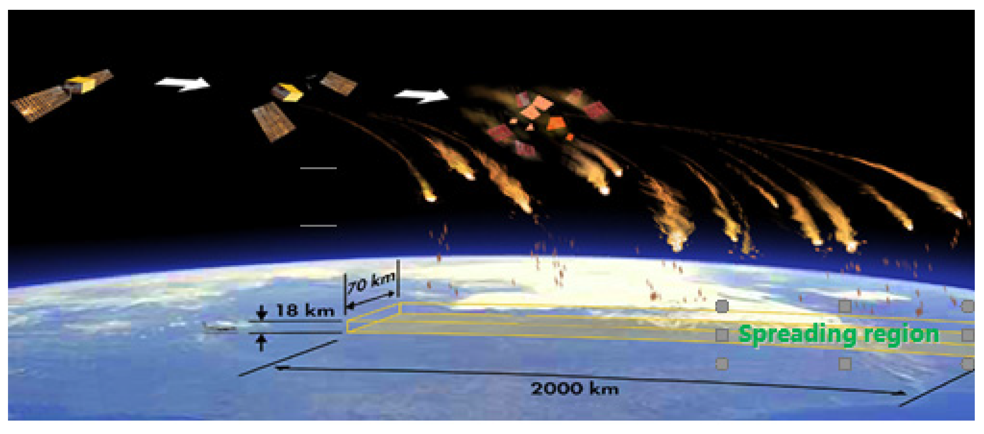
:1. Introduction
2. Physical Models and Numerical Methods
2.1. Governing Equations
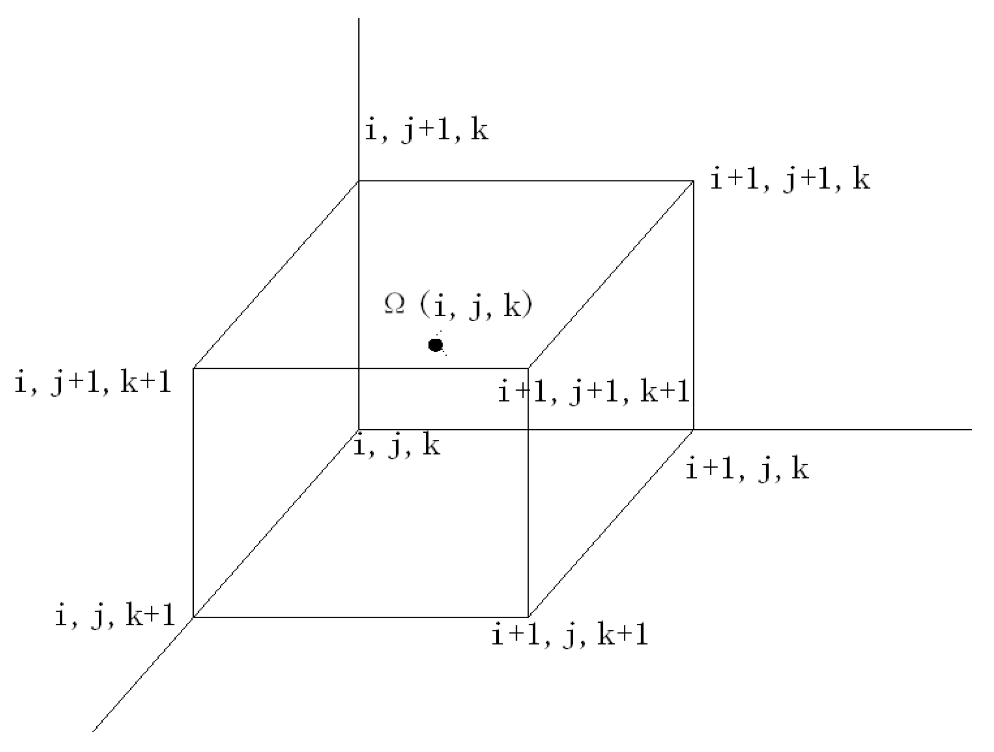
2.2. Finite Volume Method
2.3. Spatial Discrete Scheme
2.4. Time Marching Method
3. Model and Grid
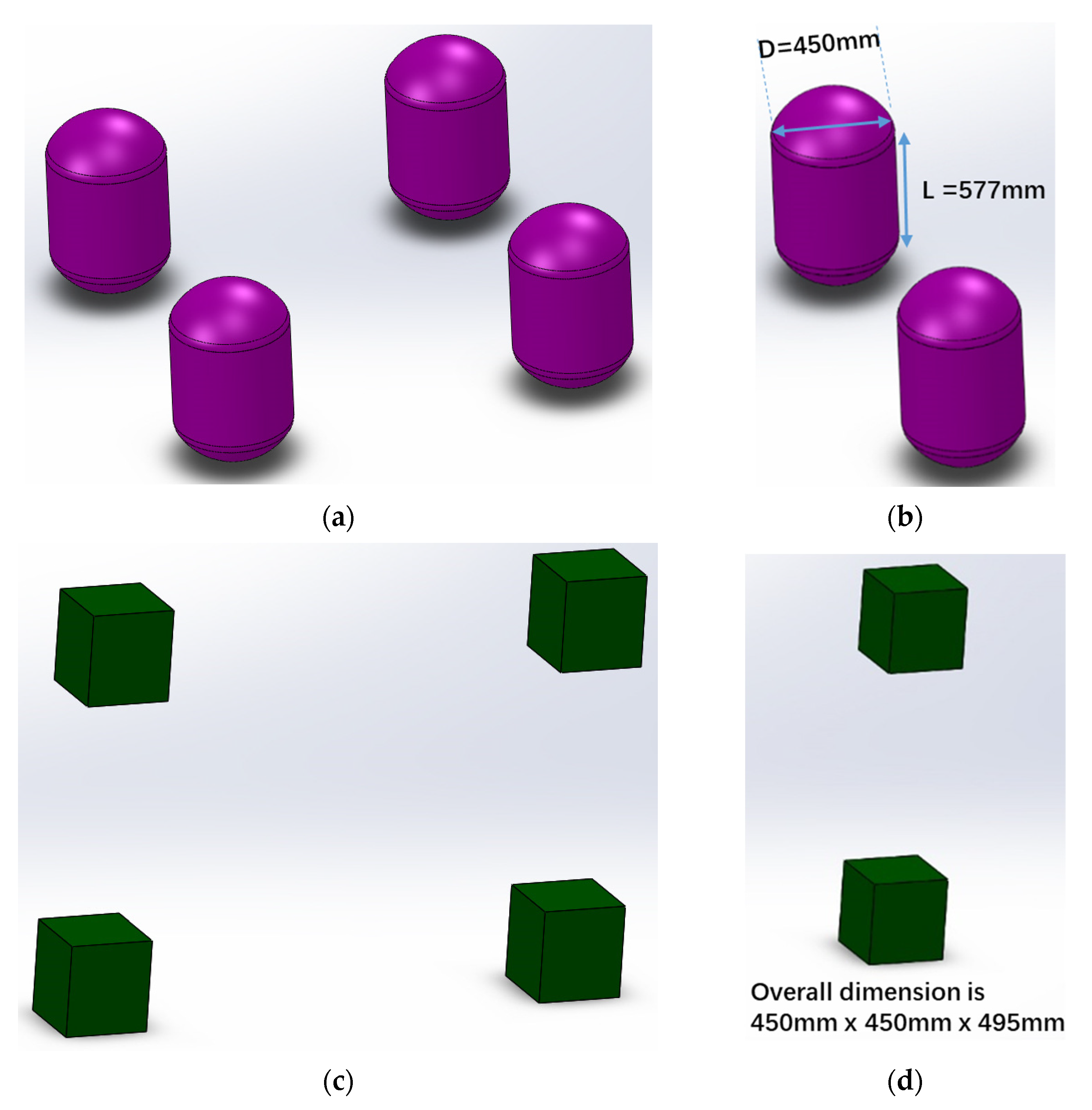
3.1. Computable Model and Computational Conditions
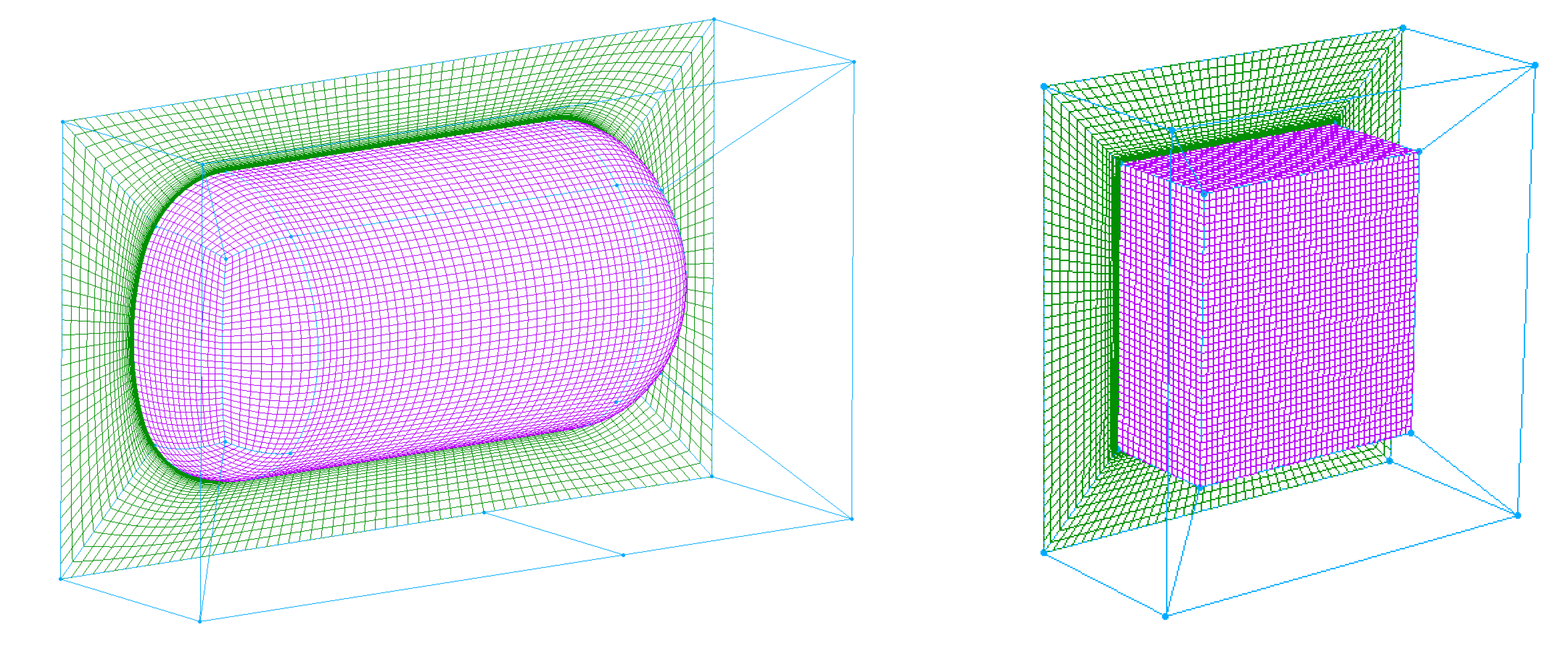
3.2. Grid Generation Method for Multi-Body Flow Field around Irregular Disintegration
3.3. Grid Sensitivity Test
4. Numerical Simulation and Analysis on Flows around Irregular Multi-Debris in Near Space
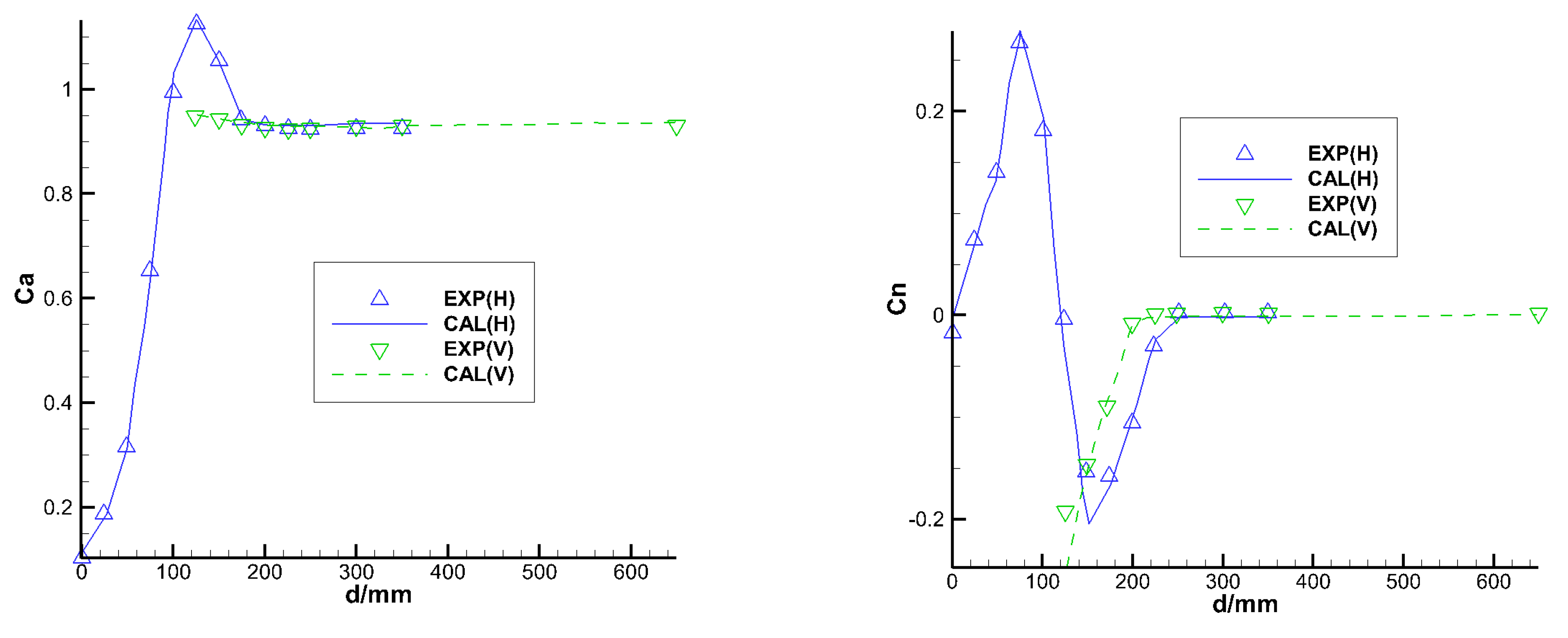
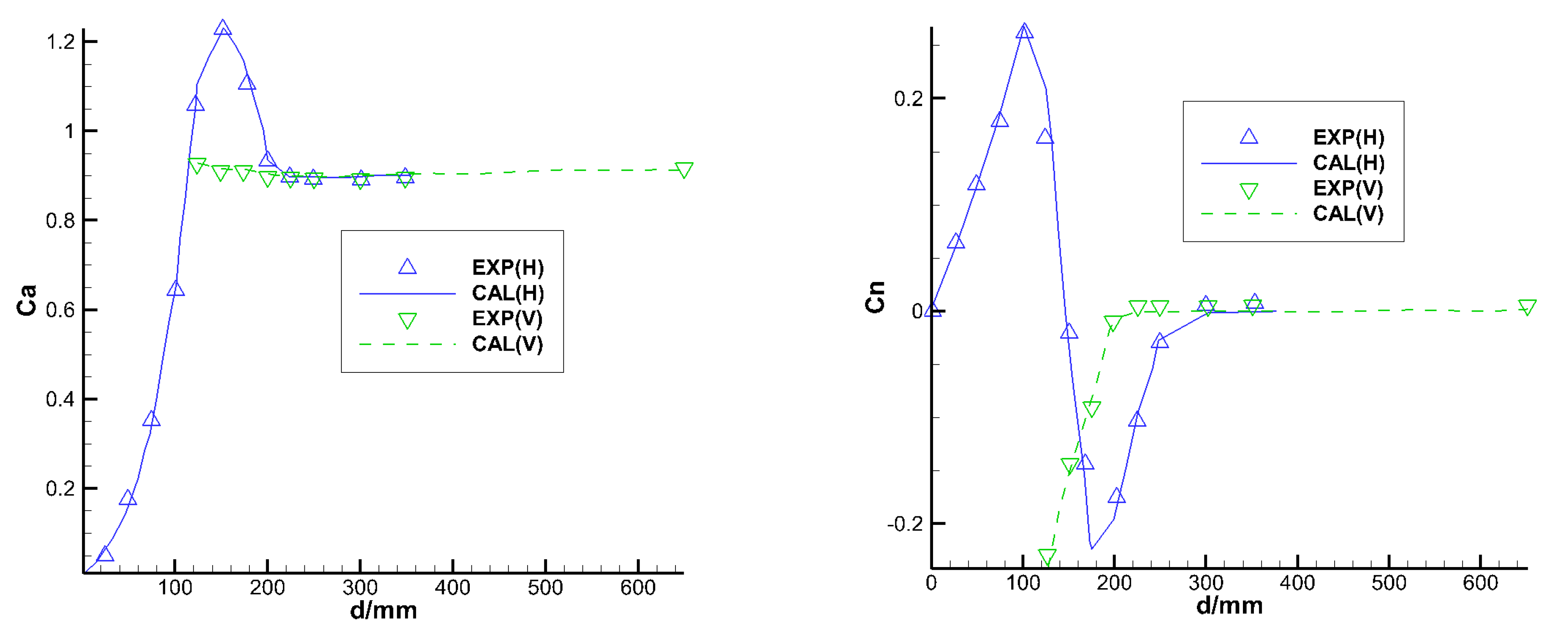
4.1. Validation/Verification of Numerical Algorithm
4.2. Numerical Simulation and Analysis on Flows around Irregular Multi-Debris in Near Space
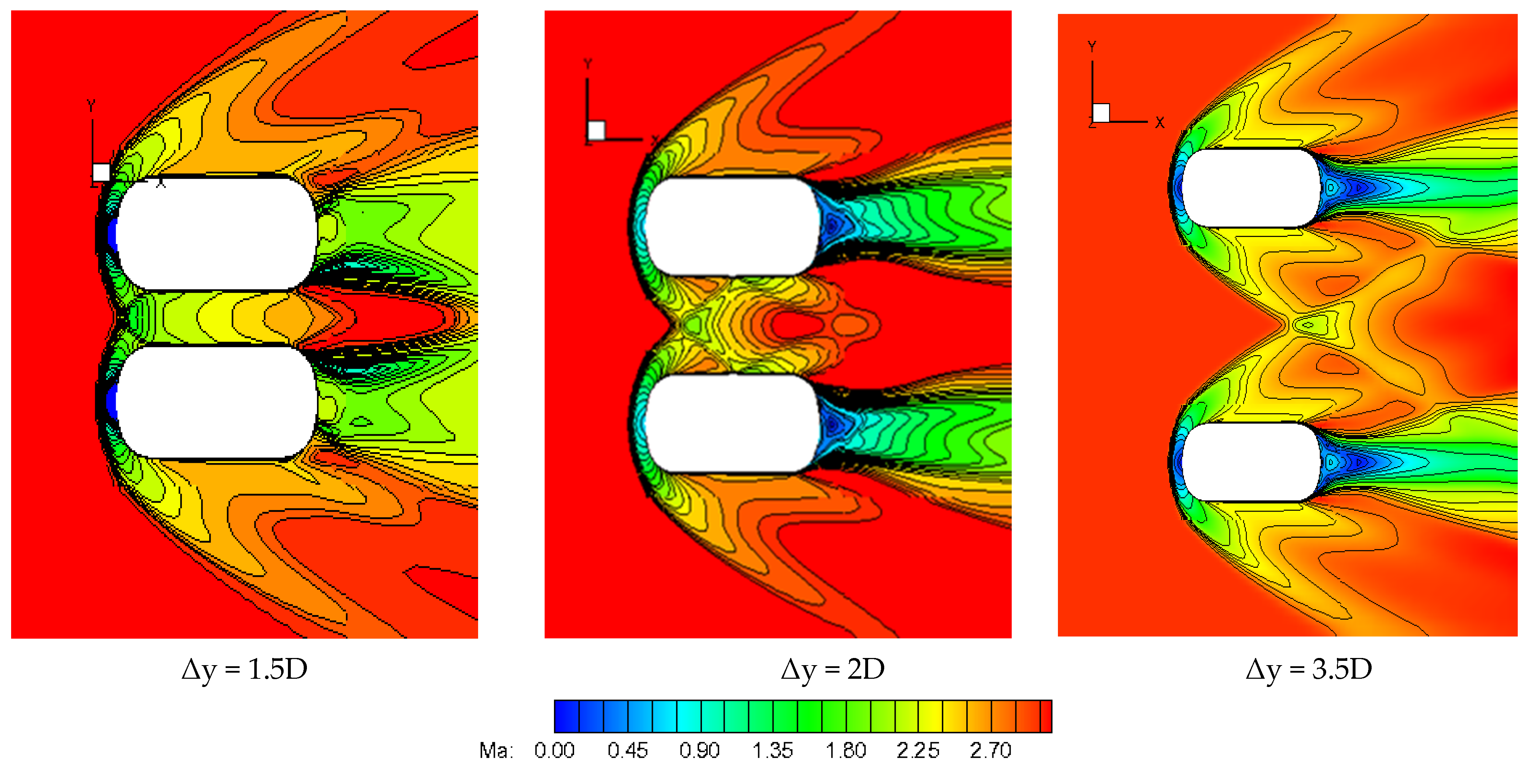
4.2.1. Numerical Simulation and Analysis on Flow around Side-by-Side Propelling Cylinders in Near Space
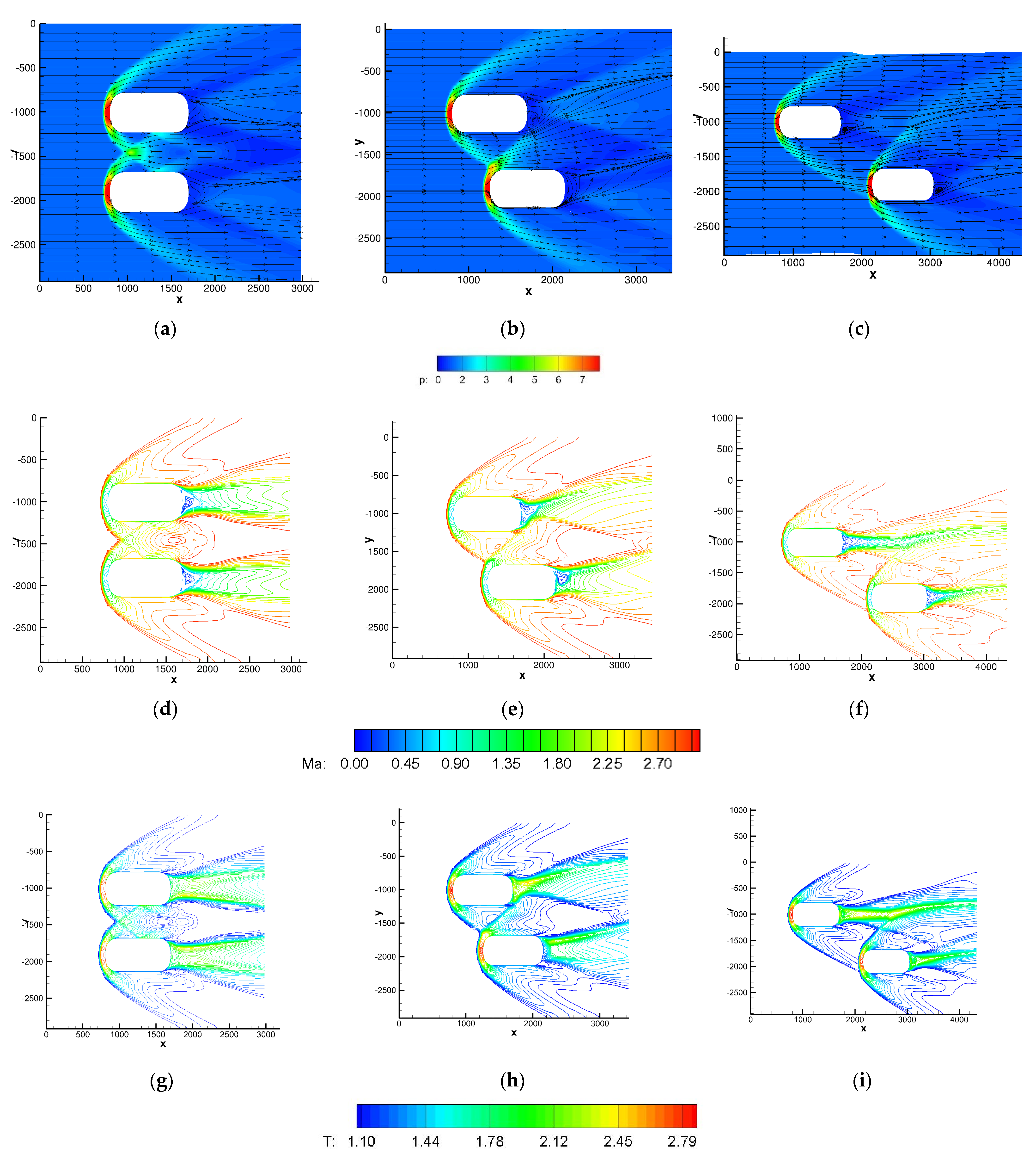
4.2.2. Numerical Simulation and Analysis on the Flow around Staggered Propulsion Cylinders in near Space
4.2.3. Numerical Simulation and Analysis on Flows around Paralleled Placed Propulsion Cylinder Bottles and Cryostats
5. Conclusion and Expectation
Author Contributions
Funding
Institutional Review Board Statement
Informed Consent Statement
Data Availability Statement
Conflicts of Interest
References
- Hoyt, R.P.; Forward, R.L. Performance of the Terminator Tether for autonomous deorbit of LEO spacecraft, AIAA 99-2839. In Proceedings of the 35th AIAA/ASME/SAE/ASEE Joint Propulsion Conference & Exhibit, Minnesota, MN, USA, 20–24 June 1999. [Google Scholar]
- Savio, P.; Eric, C.S.; Ioannis, N.; Thomas, E.S.; Graham, V.C. Nonequilibrium flow through porous thermal protection materials, Part II: Oxidation and pyrolysis. J. Comput. Phys. 2019, 380, 427–441. [Google Scholar]
- Romero, J.; Crabill, J.; Watkins, J.E.; Witherden, F.D.; Jameson, A. ZEFR: A GPU-accelerated high-order solver for compressible viscous flows using the flux reconstruction method. Comput. Phys. Commun. 2020, 250, 107169. [Google Scholar] [CrossRef]
- Fang, M.; Li, Z.H.; Li, Z.H.; Li, C.X. DSMC Approach for Rarefied Air Ionization during Spacecraft Reentry. Commun. Comput. Phys. 2018, 23, 1167–1190. [Google Scholar] [CrossRef]
- Koblitz, A.R.; Lovett, S.; Nikiforakis, N.; Henshaw, W.D. Direct numerical simulation of particulate flows with an overset grid method. J. Comput. Phys. 2017, 343, 414–431. [Google Scholar] [CrossRef]
- Lakshminarayan, V.K.; Sitaraman, J.; Roget, B.; Wissink, A.M. Development and validation of a multi-strand solver for complex aerodynamic flows. Comput. Fluids 2017, 147, 41–62. [Google Scholar] [CrossRef] [Green Version]
- Angelidis, D.; Chawdhary, S.; Sotiropoulos, F. Unstructured Cartesian refinement with sharp interface immersed boundary method for 3D unsteady incompressible flows. J. Comput. Phys. 2016, 325, 272–300. [Google Scholar] [CrossRef] [Green Version]
- Mittal, R.; Dong, H.; Bozkurttas, M.; Najjar, F.M.; Vargas, A.; Loebbecke, A. A versatile sharp interface immersed boundary method for incompressible flows with complex boundaries. J. Comput. Phys. 2008, 227, 4825–4852. [Google Scholar] [CrossRef] [PubMed] [Green Version]
- Lv, X.; Zhao, Y.; Huang, X.Y.; Xia, G.H.; Wang, Z.J. An efficient parallel/unstructured-multigrid preconditioned implicit method for simulating 3D unsteady compressible flows with moving objects. J. Comput. Phys. 2006, 215, 661–690. [Google Scholar] [CrossRef]
- Li, Z.H.; Liang, J.; Li, Z.H.; Li, H.Y.; Wu, J.L.; Dai, J.W.; Tang, Z.G. Simulation methods of aerodynamics covering various flow regimes and applications to aerodynamic characteristics of re-entry spacecraft module. Acta Aerodyn. Sin. 2018, 36, 826–847. [Google Scholar]
- Xu, G.W.; Yang, Y.J.; Zhou, W.J. Investigation on ablation effect of return capsule during reentry process. Acta Aerodyn. Sin. 2017, 35, 101–107. [Google Scholar]
- Fang, F.; Zhou, L.; Li, Z.H. A comprehensive anaylysis of aerodynamics re-entry Earth’s atmosphere surroundings. Acta Aeronaut Astronaut Sin. 2015, 36, 24–38. [Google Scholar]
- Lu, Y.D.; Li, Q.; Geng, Y.F.; Liu, X.; Gao, J.; He, X.Y. Aerodynamic design and verification technology for the circumlunar free return and reentry flight vehicle. Sci. Sin. Technol. 2015, 45, 132–138. [Google Scholar]
- Lv, J.M.; Pan, H.L.; Miao, W.B.; Cheng, X.L. Impact of chemical non-equilibrium effect on aerodynamic characteristics of reentry capsules. Spacecr. Recovery Remote Sens. 2014, 35, 11–19. [Google Scholar]
- Li, Y.L.; Qi, F.R. Optimization and implementation of China SHENZHOU spaceship’s system and return technology scheme. Spacecr. Recovery Remote Sens. 2012, 32, 1–13. [Google Scholar]
- Tang, X.W.; Zhang, S.Y.; Dang, L.N.; Shi, W.B.; Li, Z.H. Discussion on unconventional reentry/entry. Spacecr. Recovery Remote Sens. 2015, 36, 11–21. [Google Scholar]
- Li, Z.H.; Peng, A.P.; Ma, Q.; Shi, W.B.; Tang, X.W.; Dang, L.N.; Jiang, X.Y. Study and application of deformation failure disintegration algorithm for large-scale spacecraft reentry aerodynamic coupling structure. Man SPA 2020, 26, 403–417. [Google Scholar]
- Tang, X.W.; Li, S.X.; Shi, W.B.; Dang, L.N.; Li, Z.H. Disintegration modeling of spacecraft during reentry fall and primal strategy of analyzing and forecasting. Man SPA 2020, 26, 574–582. [Google Scholar]
- Lemmens, S.; Funke, Q.; Krag, H. On-Ground Casualty Risk Reduction by Structural Design for Demise. Adv. Space Res. 2015, 55, 2592–2606. [Google Scholar] [CrossRef]
- Balakrishnan, D.; Kurian, J. Material Thermal Degradation Under Reentry Aerodynamic Heating. J. Spacecr. Rocket. 2014, 51, 1319–1328. [Google Scholar] [CrossRef]
- Liang, J.; Li, Z.H.; Li, X.G.; Shi, W.B. Monte Carlo Simulation of Spacecraft Reentry Aerothermodynamics and Analysis for Ablating Disintegration. Commun. Comput. Phys. 2018, 23, 1037–1051. [Google Scholar] [CrossRef]
- Gao, X.L.; Li, Z.H.; Chen, Q.; Ding, D.; Peng, A.P. Research on short-term orbit prediction method for large-scale spacecraft at end of its life during uncontrolled flight. Man SPA 2020, 26, 566–573. [Google Scholar]
- Jiang, X.Y.; Dang, L.N.; Li, Z.H.; Li, S.H.; Tang, X.W. Analysis and research on scattered range of irregular debris for uncontrolled reentry disintegration of spacecraft. Man SPA 2020, 26, 436–442. [Google Scholar]
- Li, D.; He, Y.L.; Liu, S.; Yu, H.C.; Meng, X.F.; Li, Z.H. Study on numerical prediction of falling point distribution for near space spacecraft debris in continuous flow area. Man SPA 2020, 26, 550–556. [Google Scholar]
- Li, Z.; Peng, A.P.; Ma, Q.; Dang, L.N.; Tang, X.W.; Sun, X.Z. Gas-Kinetic Unified Algorithm for Computable Modeling of Boltzmann Equation and Application to Aerothermodynamics for Falling Disintegration of Uncontrolled Tiangong-No.1 Spacecraft. Adv. Aerodyn. 2019, 1, 4. [Google Scholar] [CrossRef] [Green Version]
- Peng, A.P.; Li, Z.H.; Wu, J.L.; Jiang, X.Y. Implicit gas-kinetic unified algorithm based on multi-block docking grid for multi-body reentry flows covering all flow regimes. J. Comput. Phys. 2016, 327, 919–942. [Google Scholar] [CrossRef] [Green Version]
- Peng, A.P.; Li, Z.H.; Wu, J.L.; Jiang, X.Y. An application of implicit gas-kinetic unified algorithm based on multiblock patched grid. Chin. J. Theor. Appl. Mech. 2016, 48, 95–101. [Google Scholar]
- Wu, J.L.; Peng, A.P.; Li, Z.H.; Fang, M. Multi-block patched mesh in gas-kinetic unified algorithm. Acta Aerodyn. Sin. 2015, 33, 624–630. [Google Scholar]
- Li, Z.H.; Ma, Q.; Cui, J.Z. Multi-scale modal analysis for axisymmetric and spherical symmetric structures with periodic configurations. Comput. Methods Appl. Mech. 2017, 317, 1068–1101. [Google Scholar] [CrossRef]
- Li, Z.H.; Ma, Q.; Cui, J.Z. Second-order two-scale finite element algorithm for dynamic thermos-mechanical coupling problem in symmetric structure. J. Comput. Phys. 2016, 314, 712–748. [Google Scholar] [CrossRef] [Green Version]
- Li, Z.H.; Jiang, X.Y.; Wu, J.L.; Xu, J.X.; Bai, Z.Y. Study on high performance parallel algorithm for spacecraft re-entry aerodynamics in the whole of flow regimes using boltzmann model equation. Chin. J. Comput. 2016, 39, 1801–1811. [Google Scholar]
- Li, Z.H.; Peng, A.P.; Wu, J.L.; Ma, Q.; Tang, X.W.; Liang, J. Gas-Kinetic Unified Algorithm for Computable Modeling of Boltzmann Equation for Aerothermodynamics during Falling Disintegration of Tiangong-type Spacecraft. In Proceedings of the 31st Intern. Symposium on Rarefied Gas Dynamics, Glasgow, UK, 23–27 July 2018. [Google Scholar]
- Wilcox, D.C. Turbulence Modeling for CFD, 3rd ed.; DCW Industries Inc.: La Canada, CA, USA, 2006; pp. 243–249. [Google Scholar]
- Gary, C.C.; Roy, P.K.; Bharat, K.S. Multidisciplinary and multi-scale computational field simulations—Algorithms and applications. Math. Comput. Simul. 2007, 75, 161–170. [Google Scholar]
- Nathan, C.P.; Davy, M.B.; Wei, S. Parallel computing of overset grids for aerodynamic problems with moving objects. Prog. Aerosp. Sci. 2000, 36, 117–172. [Google Scholar]
- Kiris, C.C.; Housman, J.A.; Barad, M.F.; Brehm, C.; Sozer, E.; Moini-Yekta, S. Computational framework for Launch, Ascent, and Vehicle Aerodynamics (LAVA). Aerosp. Sci. Technol. 2016, 55, 189–219. [Google Scholar] [CrossRef]
- Yang, X.L.; Wang, J.Y.; Zhou, Y.; Sun, K. Assessment of radiative heating for hypersonic earth reentry using nongray step models. Aerospace 2022, 9, 219. [Google Scholar] [CrossRef]
- Zhang, J.; Tan, J.J.; Geng, J.H. Numerical simulation of 2D mult-i bodies with moving boundaries. Acta Aerodyn. Sin. 2003, 21, 449–453. [Google Scholar]
- Mongelluzzo, G.; Esposito, F.; Cozzolino, F.; Franzese, G.; Ruggeri, A.C.; Porto, C.; Molfese, C.; Scaccabarozzi, D.; Saggin, B. Design and CFD Analysis of the Fluid Dynamic Sampling System of the “MicroMED” Optical Particle Counter. Sensors 2019, 19, 5037. [Google Scholar] [CrossRef] [Green Version]
- Roe, P.L. Approximate Riemann solvers, parameter vectors and difference schemes. J. Comput. Phys. 1981, 43, 357–372. [Google Scholar] [CrossRef]
- Yoon, S.; Jameson, A. Lower-Upper Symmetric-Gauss-Sediel Method for the Euler and Navier-Stokes Equations; AIAA Paper; AIAA: Reston, VA, USA, 1988; pp. 1025–1026. [Google Scholar]
- Shen, Y.; Wang, B.; Zha, G. Comparison Study of Gauss-Seidel Line Iteration Method for External and Internal Flows; AIAA Paper; AIAA: Reston, VA, USA, 2012; pp. 2007–4332. [Google Scholar]
- Thakur, S.; Wright, J.; Shyy, W.; Liu, J.; Ouyang, H.; Vu, T. Development of pressure-based composite multigrid methods for complex fluid flows. Prog. Aerosp. Sci. 1996, 32, 313–375. [Google Scholar] [CrossRef]
- Li, X.G.; Yang, Y.G.; Li, Z.H.; Pi, X.C. Design methods of the small size strain gauge balance. J. Exp. Fluid Mech. 2013, 27, 78–82. [Google Scholar]


| Case A (Coarse) | Case B (Medium) | Case C (Fine) | |
|---|---|---|---|
| Grid Reynolds Number | 200 | 100 | 50 |
| Total Grid Number | 560,651 | 989,901 | 1,845,371 |
| Case A (Coarse) | Case B (Medium) | Case C (Fine) | ||
|---|---|---|---|---|
| Propulsion bottle | Axial force Coefficients | 0.175 | 0.189 | 0.189 |
| Normal force Coefficients | 0.186 × 10⁻⁵ | 0.197 × 10⁻⁵ | 0.197 × 10⁻⁵ | |
| Lock cabinet | Axial force Coefficients | 0.079 | 0.088 | 0.088 |
| Normal force Coefficients | 0.777 × 10⁻⁶ | 0.828 × 10⁻⁶ | 0.839 × 10⁻⁶ | |
| Δy | 1.5D | 2D | 3.5D |
|---|---|---|---|
| Minimum distance | 109 mm | 109 mm | 109 mm |
| position of shocks intersection | X = −26 mm | X = 143 mm | X = 640 mm |
| Δy | 1.5D | 2D | 3.5D |
|---|---|---|---|
| Axial force coefficient | 0.0880 | 0.0873 | 0.0755 |
| Normal force coefficient | 0.0367 | 0.0322 | 1.055 × 10⁻⁴ |
| Δx | 0 | D | 3D | |
|---|---|---|---|---|
| Propulsion bottle (front) | Axial force coefficient | 0.0873 | 0.0872 | 0.0881 |
| Normal force coefficient | 0.0322 | 1.147 × 10⁻⁴ | 5.3974 × 10⁻⁵ | |
| Propulsion bottle (back) | Axial force coefficient | 0.0873 | 0.0920 | 0.1001 |
| Normal force coefficient | 0.0322 | 0.0157 | 4.8940 × 10⁻³ | |
| Δy | 1.5D | 3D | 4.5D | |
|---|---|---|---|---|
| Propulsion bottle | Axial force coefficients | 0.098 | 0.187 | 0.189 |
| Normal force coefficients | 0.197 × 10⁻¹ | 0.662 × 10⁻⁵ | 0.197 × 10⁻⁵ | |
| Cryostat | Axial force coefficients | 0.188 | 0.087 | 0.088 |
| Normal force coefficients | 0.217 × 10⁻¹ | 0.688 × 10⁻⁴ | 0.839 × 10⁻⁶ | |
Publisher’s Note: MDPI stays neutral with regard to jurisdictional claims in published maps and institutional affiliations. |
© 2022 by the authors. Licensee MDPI, Basel, Switzerland. This article is an open access article distributed under the terms and conditions of the Creative Commons Attribution (CC BY) license (https://creativecommons.org/licenses/by/4.0/).
Share and Cite
Han, Z.; Li, Z.; Bai, Z.; Li, X.; Zhang, J. Study on Numerical Algorithm of the N-S Equation for Multi-Body Flows around Irregular Disintegrations in Near Space. Aerospace 2022, 9, 347. https://0-doi-org.brum.beds.ac.uk/10.3390/aerospace9070347
Han Z, Li Z, Bai Z, Li X, Zhang J. Study on Numerical Algorithm of the N-S Equation for Multi-Body Flows around Irregular Disintegrations in Near Space. Aerospace. 2022; 9(7):347. https://0-doi-org.brum.beds.ac.uk/10.3390/aerospace9070347
Chicago/Turabian StyleHan, Zheng, Zhihui Li, Zhiyong Bai, Xuguo Li, and Jiazhong Zhang. 2022. "Study on Numerical Algorithm of the N-S Equation for Multi-Body Flows around Irregular Disintegrations in Near Space" Aerospace 9, no. 7: 347. https://0-doi-org.brum.beds.ac.uk/10.3390/aerospace9070347