Article

Seasonal Dynamics of Soil Moisture in an Integrated-Crop-Livestock-Forestry System in Central-West Brazil

1
Institute of Agricultural Sciences in the Tropics (Hans-Ruthenberg-Institute), University of Hohenheim, 70599 Stuttgart, Germany
2
Brazilian Agricultural Research Corporation, Embrapa Beef Cattle, Rádio Maia Avenue, 830, Campo Grande—MS, CEP 79106-550, Brazil
*
Author to whom correspondence should be addressed.
Submission received: 30 January 2021 / Revised: 5 March 2021 / Accepted: 7 March 2021 / Published: 12 March 2021

Abstract

:
Integrated-crop-livestock-forestry (ICLF) systems are currently promoted as a measure for sustainable intensification of agricultural production. However, due to complex interactions among ICLF components, we are still lacking evidence about the system’s resilience regarding water availability, especially for regions characterized by pronounced wet and dry seasons and frequent droughts. For a mature ICLF system in the Cerrado biome of central-west Brazil comprising rows of eucalyptus trees (Eucalyptus grandis x Eucalyptus urophylla, H13 clone) at a spacing of 22 m in combination with Brachiaria brizantha cv. BRS Piatã pasture we continuously measured soil moisture (SM) until 1 m depth and supported this data with measurements of photosynthetically active radiation (PAR) and aboveground green grass biomass (AGBM) across transects between the tree rows for almost two years. Across the seasons a distinct gradient was observed with SM being lower close to the tree rows than in the space between them. During winter SM decreased to critical values near the tree lines in the topsoil. During spring and summer, incident PAR was 72% and 86% lower close to the trees than at the center point. For autumn and winter PAR was more evenly distributed between the tree rows due to inclination with notably up to four times more radiation input near the tree lines compared to spring and summer. AGBM showed a clear distribution with maximum values in the center and about half of the biomass close to the tree rows. Our data suggest that, restrictions in AGBM accumulation shifted among seasons between water limitations in winter and light limitations during summer. Interestingly, SM changes during wetting and drying events were most pronounced in subsoils near the tree rows, while the topsoil showed much less fluctuations. The subsoil in central position showed the lowest SM dynamics in response to drought maintaining a relative high and constant SM content, therefore functioning as important water reservoirs likely improving the resilience of the system to drought stress. Results of this study could help to improve management and the design of ICLF systems in view of sustainability and resistance to (water) crises but should be further supported by in depth analysis of soil water dynamics as affected by climate gradients, soil types and different management practices.

1. Introduction

The Brazilian Savannah, also known as the Cerrado, covers an area of 204.7 million ha (about 22% of the Brazilian territory). In the last few decades, about 50% of the natural Cerrado vegetation has been replaced by agricultural crops and pastures [1,2,3]. According to Macedo [4], the planted pasture area in the Cerrado amounts to 60 million ha, of which 85% (51 million ha) is planted with Brachiaria grasses. It is estimated that more than 70% of the cultivated pastures in Brazil are degraded, or are at some stage of degradation, especially in the Cerrado region [5]. The main causes for pasture degradation in Brazil are overstocking with cattle and insufficient replenishment of soil nutrients [5]. Integrated-crop-livestock-forestry (ICLF) systems combine crop and livestock in succession, rotation or by intercropping with trees in the same area [6], and are a reliable alternative to restore degraded pastures [7]. For this reason, integrated systems are currently considered an option for sustainable intensification, improving food security and environmental stability [8,9,10]. A significant benefit of ICLF systems is soil conservation, which reduces erosion, maintains or increases soil organic matter, and improves soil structure and porosity, resulting in increased infiltration and water holding capacity [11,12]. Increased soil water infiltration and water storage in ICLF systems led to their promotion as a promising land use option to reduce drought impacts on agricultural production, which may be more frequent due to climate change [13].
The presence of trees in ICLF systems affects the understory Brachiaria pasture by changing microclimatic conditions, like reducing photosynthetically active radiation (PAR), and wind speed [14]. These changes have an impact on evapotranspiration and biomass production of the pasture and, consequently, soil moisture content [3,15,16]. The effect of the trees on the understory microclimate depends on the distance to the tree rows, and there are significant differences in quality and amount of solar radiation due to the spatial arrangement and density of the trees [3,15,17]. According to Bruner and Belesky [18], the reduction of PAR is the main constraint for aboveground biomass production, provided sufficient soil moisture availability.
Despite being considered a key indicator of how ICLF systems affect ecological processes, soil water dynamics in literature have not been consistently analyzed, and continuous observation of seasonal soil water dynamics are mostly unaddressed. Since soil moisture of complex ecosystems is influenced by a number of factors, several additional parameters need to be taken into account to create a comprehensive understanding of the interlinked processes, such as light, rainfall interception, SM dynamics, and biomass productivity. This is further complicated by combining different components of crops, trees, and animals in diverse environments and under variable management. Using the example of a mature ICLF system in Campo Grande (in the state of Mato Grosso do Sul), this study aims to analyze system’s water dynamics in characteristic seasons of the Cerrado ecotone complemented by simultaneous analysis of (1) photosynthetically active radiation (PAR) received at grass canopy level, (2) soil moisture (SM), and (3) aboveground green grass biomass (AGBM) between the tree rows and seasons in an ICLF system. We hypothesize that the seasonal impact alters interdependencies among the measured parameters, allowing for improved understanding of resilience and adaptive capacity of ICLF systems relating to variable environments triggered by climate variability or change.

2. Materials and Methods

2.1. Experimental Site

The study was carried out on the experimental sites of EMBRAPA Beef Cattle (Brazilian Agricultural Research Corporation), located in Campo Grande, state of Mato Grosso do Sul, Brazil (20°24′54.9″ S, 54°42′25.8″ W, altitude 530 m). The climate of the area is a tropical savannah Aw climate (Köppen) with a mean annual temperature of 22.6 °C. The study area is characterized by four defined seasons: summer (December–February), autumn (March–May), winter (June–August), spring (September–November), with the peak of the rainy season during the summer months and the peak of the dry season during the winter months (Figure 1). About 70% of the mean annual rainfall, around 1560 mm, falls within the rainy season, and the remaining 30% within the dry season. Temperature, relative air humidity, solar radiation, wind speed, and precipitation were monitored by a nearby meteorological station operated by EMBRAPA Beef Cattle. Furthermore, rainfall was monitored at one sampling point (P6S) between the trees at the experimental site using a IM523 rain gauge by iMetos connected to an event/temp data logger (HOBO Pendant Data Logger Event and Temperature UA-003), as well as along a transect of five sampling points between the tree rows with commercial rain gauges.
According to the World Reference Base for Soil Resources [19], the soil of the study area is classified as a Ferralsol. Soil samples were taken in 10, 20, 30, 40, 60 and 100 cm depth with coring rings (10 cm−3). The soil profile was created using an excavator in February 2017. The 1.2 m-deep and 1 m-wide hole was dug in Rep 2 (Figure 2). For each depth, soil samples were taken with a coring ring in three of the four soil profile walls, resulting in three replicates per depth. The soil had a sandy clay texture (55% sand, 6% silt, 39% clay), a bulk density of 1.15 g cm−3, a usable field capacity between soil moisture values of 15.5 Vol% (pF 4.2, permanent wilting point) and 42.5 Vol% (pF 1.8, field capacity), a hydraulic conductivity of 59.2 cm day−1 and a pH value (measured in water) of 4.5.

2.2. ICLF System

The ICLF system was established in 2008. The area was prepared using light to heavy tillage and limestone/gypsum application (3 and 1 t ha−1, respectively) to increase the pH and to improve P availability for the crops. In early November 2008, NPK fertilizer (5:25:15) was applied at a rate of 400 kg ha−1, followed by levelling with a disk harrow. The amount of fertilizer was determined through chemical soil analysis and applied according to the experience and guidelines of EMBRAPA Beef cattle. In late November 2008, the crop component (Glycine max cv. BRS 255RR), and in January 2009, the tree component (Eucalyptus grandis x Eucalyptus urophylla, H13 clone), were planted. The eucalyptus seedlings were transplanted in east–west oriented rows. Each replicate had an area of 1.4 ha, and consisted of two single tree rows at a distance of 22 m and 2 m distance between the trees within each row, resulting in a tree density of 227 trees ha−1 (Figure 2). After the soybean harvest in April 2009, the pasture component (Brachiaria brizantha cv. BRS Piatã) was established and beef cattle (Nellore heifers) were introduced to the system as the trees reached a diameter at breast height, at least 60 mm. The cattle grazed at varying stocking rates depending on biomass production in order to keep the height of the pasture at approximately 35 cm (put and take method). The management of the ICLF system involved a crop rotation strategy every four years (i.e., cultivation of soybean as a crop for five months) followed by three and a half years of Brachiaria brizantha cv. BRS Piatã pasture. For this study, data was collected in the third year after pasture establishment during the second pasture cycle of the ICLF system from November 2015 until August 2017 at tree height of about 25 to 27 m. In January 2016, 50 kg N ha−1 (in the form of urea) and 300 kg NPK ha−1 (0:20:20) were applied to the pasture.

2.3. PAR, SM and AGBM

Photosynthetically active radiation (PAR), soil moisture (SM) and aboveground green grass biomass (AGBM) were measured along a transect of five sampling points between tree rows to assess the shading and soil moisture gradient created by the trees. These five sampling points were: P1S: 1 m and P6S: 6 m from the southern row; P1N: 1 m and P6N: 6 m from the northern row; P11: 11 m from the southern and the northern row respectively (Figure 2).
PAR (µmol m−2 s−1) was measured monthly with a Decagon AccuPAR LP-80 at clear sky, in the morning and in the afternoon directly above the grass canopy at each sample point between the tree rows, and on an open field (without any trees) beside the ICLF system. PAR values shown in this study represent means of measurements performed in the morning and afternoon.
At each sampling point in each replication, a fiberglass access tube (DeltaT Type: ALT1) of 1 m length was vertically installed for volumetric SM (Vol%) measurements with a portable DeltaT FDR (frequency domain reflectometry) PR2/6 profile probe. FDR measurements were taken weekly in depths of 10, 20, 30, 40, 60 and 100 cm. The FDR soil moisture measurements were validated against gravimetrical soil moisture measurements. Samples for gravimetrical soil moisture measurements were taken with an auger right next to every FDR access tube at the same depths where the FDR probe measurements were taken.
AGBM (g DW m−2) was quantified monthly. At each sampling point in each replication, 1 m2 of grass biomass was harvested 5 cm from the ground. All harvested biomass samples were separated into green biomass and dead biomass, dried for 48 h at 70 °C and weighed to determine the dry weight biomass per area in g m−2.

2.4. Data Analysis

Data was analyzed in a randomized complete block (three replicates) design using the generalized least squares model of R [20,21,22], with repeated measurements over time, and the seasons (spring, summer, autumn, winter) as a repeated factor. For the analysis of SM and AGBM sample points, season and block were considered as fixed effects. The most appropriate correlation structure for repeated measurements was chosen according to the Akaike Information Criterion (AIC). For AGBM the first order autoregressive (ar(1)) correlation structure was chosen. Fisher’s LSD (least significant difference) test and significance at p < 0.05 were used for the comparison of mean values. The Pearson correlation coefficient (r) between PAR and AGBM and SM and AGBM was calculated also using R [20]. To normalize data for the correlation analysis, relative values of PAR, SM and AGBM along the gradient between the tree rows were calculated.

3. Results

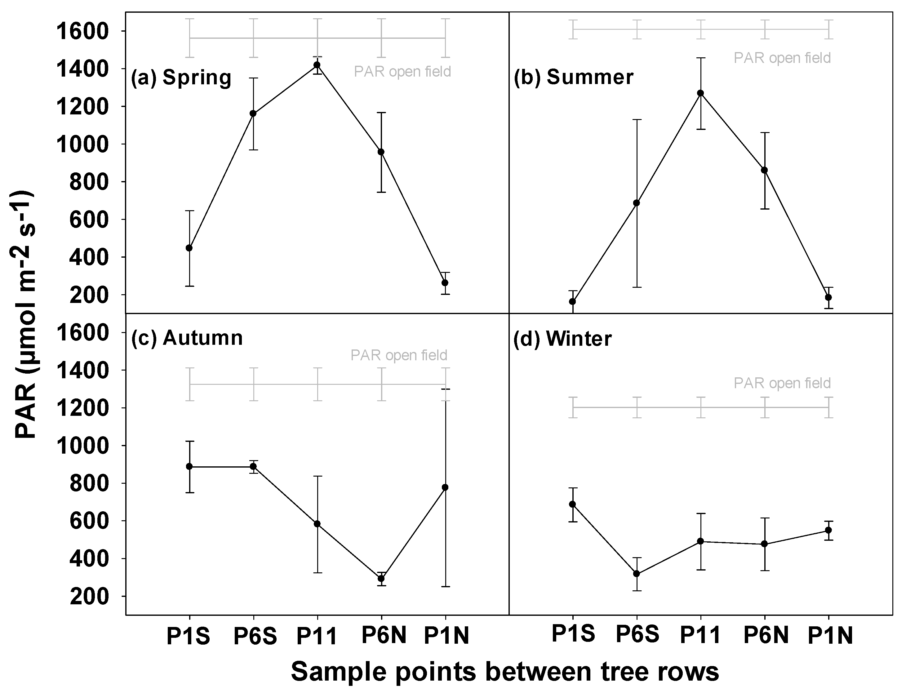
3.1. PAR between the Tree Rows during Different Seasons

PAR received by the grass canopy varied widely between the seasons, but also between the tree rows, especially in spring and summer (Figure 3). In comparison to open field measurements, P11 received 9% less PAR in spring and 21% less PAR in summer, respectively. Furthermore, in both seasons, the sample points closest to the tree rows (P1S and P1N) received with about 200 µmol m−2 s−1 even less PAR than all other sample points in winter. In winter, PAR was more evenly distributed between the sample points, with P1S receiving 43% and P6S 74% less PAR compared to the open field. In autumn, P1S and P6S received 33% less PAR compared to the open field, P11 and P1N about 50% less, and P6N 78% less. In contrast to spring and summer, in autumn and winter, the sample points P6S and P6N received even slightly more PAR than the center sample points.

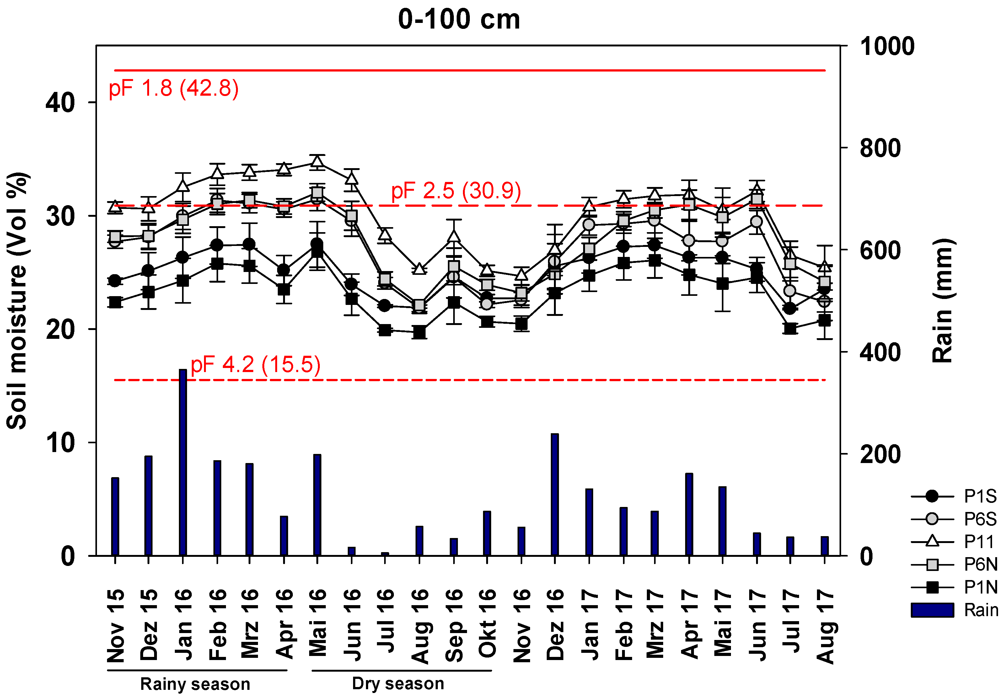
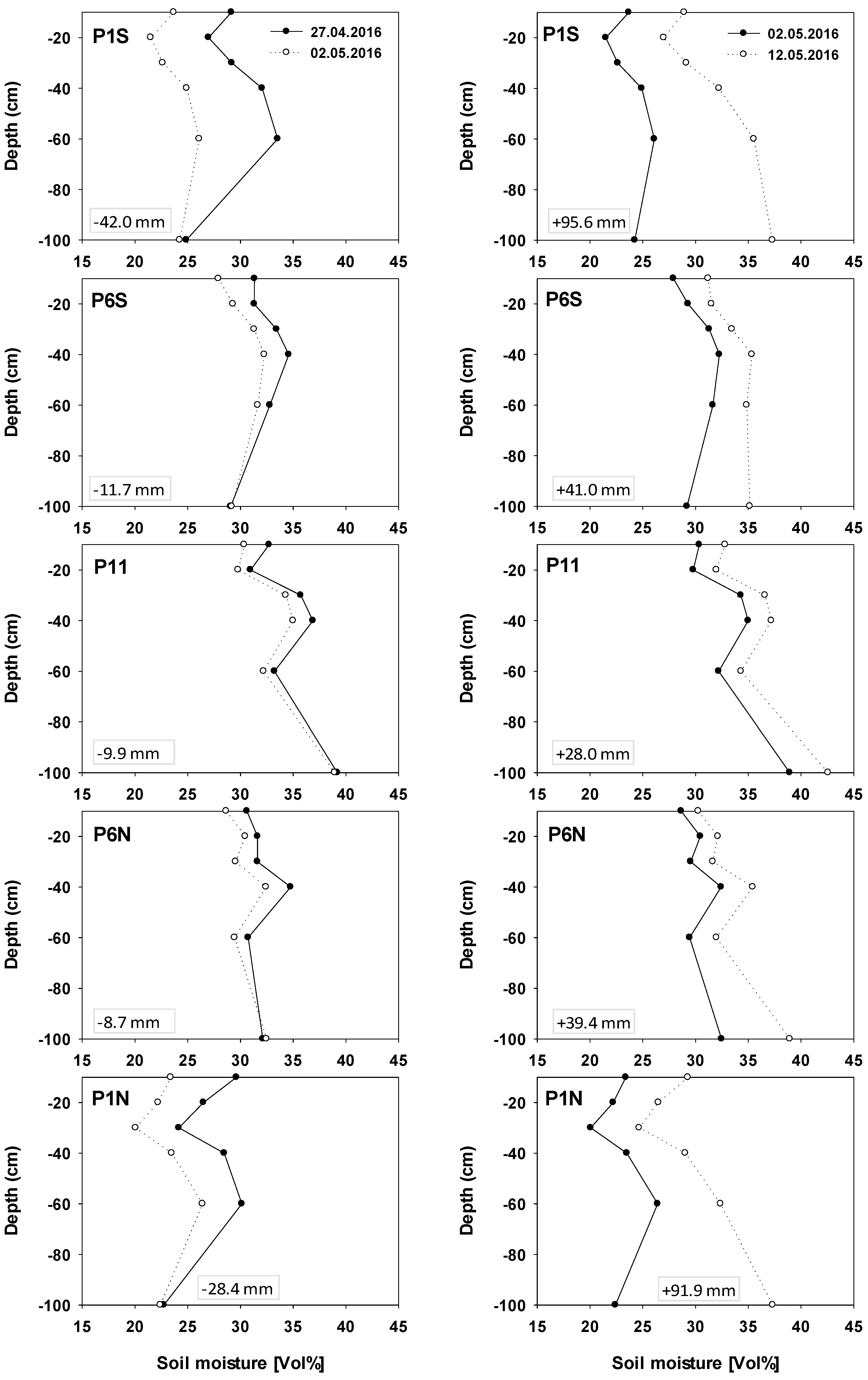
3.2. SM in ICLF between the Tree Rows during Different Seasons

Throughout the measurement period, monthly mean SM in the top 1 m soil layer was highest in the rainy season (November–April), and up to 10 Vol% lower in the dry season (May–October) for all sample points (Figure 4). On average over the sample points, SM was lowest in August 2016, with 21.1 Vol%, and highest in May 2016, with 30.5 Vol%. Between the sample points, SM was lowest at P1N, with 23.2 Vol%, followed by P1S, with 25.0 Vol%, and highest at P11, with 30.1 Vol%, on average over the measurement period. Little difference was found between P6S and P6N, which had 27.2 Vol% and 27.9 Vol% SM on average over the measurement period.
Analysis of variance revealed highly significant differences (p ≤ 0.001) between the months and between the sample points, but no significant difference between both years (Table 1).
During the first year and the second year, and at all SP, SM increased with depth, except at P6S, P11, and P6N in the first year and spring of the second year (Figure 5). At these sample points, SM decreased at depths between 40 m and 60 cm, but increased at greater depths. Throughout the profile, SM was lower during the second year compared to the first year. During both years and for all seasons, SM next to the trees (P1S and P1N) was lower compared to the center point P11, as well as P6S and P6N. Further, SM at P1S was always slightly lower than at P1N. Throughout the profile, SM was lowest during winter followed by spring, summer, and autumn during the first year, whereas during the second year, SM was lowest in spring followed by winter, summer and autumn. However, in the topsoil (10 cm to 30 cm depth), SM was lowest during winter in both years.
Analysis of variance showed significant differences in SM between years (except for 60 cm depth), seasons and sample points at all measured depths (Table 2). Whereas in the topsoil at 10 cm depth, season had the largest effect on SM, the influence of the sample point became larger with increasing soil depth.

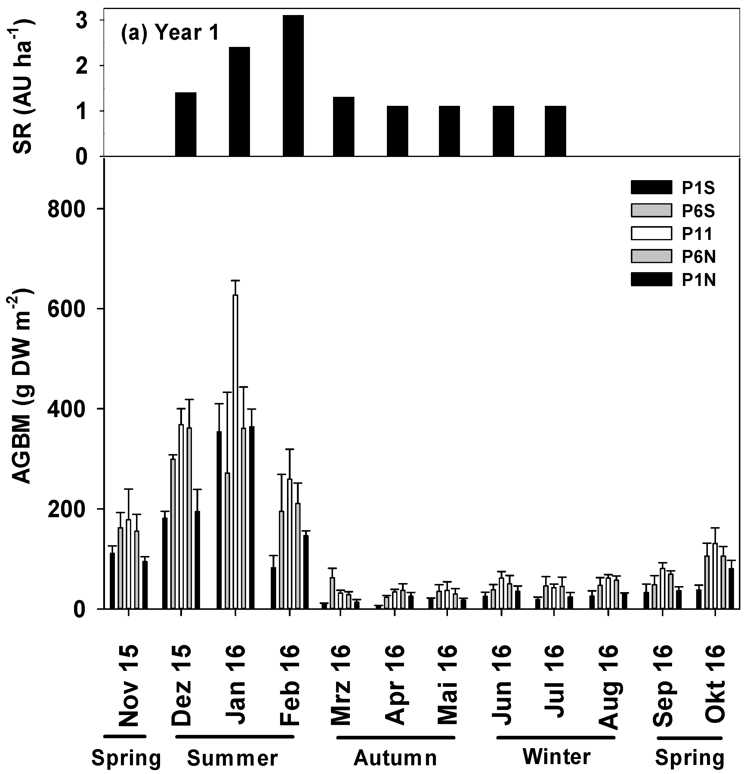
3.3. AGBM between the Tree Rows during Different Seasons

Grazing intensity differed largely between both years, with grazing activities from December until July, and the highest stocking rate (3.2 AU ha−1) in February during the first year and grazing in December only during the second year (Figure 6). Consequently, in the first year, AGBM was with 114 g DW (dry weight) m−2 on average, substantially lower than in the second year, with 297 g DM m−2.
The ANOVA showed highly significant differences (p ≤ 0.001) between both years, months and sample points (Table 3). In both years, the highest AGBM was measured in January, but in the first year, AGBM drastically decreased from February to March, whereas in the second year, AGBM decreased more slowly. The largest difference between both years was found between March and August. In both years, between most of October and February, AGBM was highest at P11, and lowest at P1S and P1N. However, between March and May in the second year, the highest AGBM was found at P1S and P6S.
AGBM was highest during summer at all sampling points in both years (Table 4). In the first year, AGBM was lowest in autumn and winter, while in the second year, it was lowest in spring and winter. In the first year, AGBM at P11 was significantly higher than at P1S and P1N during summer, autumn and winter. During spring, no significant differences between the sample points were found. In year 2, AGBM was only significantly higher at P11 than at both points close to the trees during summer, while during spring and winter, significant differences were only found between P11 and one of both measurement points close to the trees.

3.4. Correlation between PAR and AGBM and SM 0–100 cm and AGBM between the Tree Rows

In spring and summer, AGBM was closely correlated with both, PAR and SM, with higher correlation coefficients with PAR (Table 5). In autumn and winter, the correlation between PAR and AGBM was negative and not significant, whereas the correlation between SM and AGBM was positive and in winter, also highly significant.

4. Discussion

4.1. PAR, SM and AGBM Distribution throughout the Year

The trees in the ICLF system affected the amount of PAR received by the pasture, with a relative PAR reduction depending on the season and on the distance to the trees. The fact that in silvopastoral systems the pasture is shaded by the trees, is a well-known phenomenon with negative effects on both, light quantity and quality as red/far red ratio, received at the grass canopy [17,23]. The relative PAR reduction depends mostly on tree height, which was about 26 m at the beginning of our measurements and thus, led to a relatively large mean PAR reduction of 53% compared to above canopy PAR values (Table 6). Further, the magnitude of the effects depends on tree spacing, with spacing of more than 20 m between tree rows, as in our case, being beneficial for the relative light intensity in the median between tree rows [3,17]. In addition to tree height and spacing, time of day and time of year influence PAR reception at grass canopy level, related to the inclination of the sun. Light transmission at the center point between the tree rows was observed to be lower close to sunrise and sunset and during autumn and winter months [14]. In our experimental plots, PAR was reduced by more than 50% at the center point P11 during autumn and winter. Since PAR values represent means of measurements performed in the morning and afternoon, the sun did not rise above the tree canopy yet at the time of measurement during autumn and winter. However, a reduction in PAR near the trees was higher during spring and summer, whereas during autumn and winter, PAR was more evenly distributed between the tree rows. In absolute values, PAR received by the grass canopy close to the trees was up to 4 times higher in autumn and winter, than during spring and summer. Feldhake [23] observed peak levels of solar radiation under the trees at 25% cloud cover because of increased diffuse radiation. In our experiment, PAR measurements were performed only under clear sky conditions. However, we hypothesized that a high ratio of diffuse radiation between the tree rows during autumn and winter led to both, a low relative PAR reduction close to the trees in comparison to the center point P11, and higher absolute PAR value close to the trees during autumn and winter compared to spring and summer. As seasons were defined meteorologically, and not by days of solstice and equinox, spring (September–November) and summer (December–February) resulted in relatively similar PAR values. Equally, PAR distribution during autumn (March–May) and winter (June–August) were very similar.
SM over a soil depth of 0–100 cm showed a distinct seasonal dynamic closely related to rainfall pattern (Figure 4). SM was significantly lower in the second year, since precipitation was substantially lower than in the first year (1020 mm vs. 1553 mm). Further, SM in the topsoil (0–30 cm) was generally lower and more dynamic, which has also been found in a similar experimental setup by Bosi et al. [15], who related this effect to water uptake by the pasture and evaporation from the soil, especially at the beginning of a drying period. Furthermore, in the topsoil, permanent wilting point was almost reached at some measurement points. For Brachiaria brizantha, more than 80% of the roots were found in the upper 30 cm of the soil, both under full irrigation and under water deficit [24], and plant biomass was significantly decreased by water deficit, when soil water levels reached 25% of field capacity [25]. At our study site, a soil water content of 25% of field capacity equals a volumetric soil moisture of 19.4%. During winter, soil moisture at 0–30 cm was often below this threshold and, thus, negatively affected plant biomass.
Intra- and inter-annual AGBM values varied largely to intra- and inter-annual climate variability and development related senescence processes of the grass. Depending on temperature, daylength, solar radiation, and rainfall [26], canopy senescence is faster than canopy renewal during the cool and dry winter period. With regard to development, in Brazil, the cultivar Piatã starts flowering in January and February [27], influenced by changes in photoperiod that stimulates floral induction [28]. Flowering and seed development generally serve as a cue for tiller senescence in grasses [29].
Despite the lower precipitation, more AGBM was observed in the second year, due to a significantly lower grazing intensity. In the first year, the pasture was grazed starting in December, which lead to a strong decline in AGBM until March, without recovery during autumn and winter. In the second year, grazing took place only during summer and a very low stocking rate was maintained. Under the conditions of the second year AGBM still peaked during January, but declined very slowly until August. The much higher AGBM in the second year could explain the lower top-soil values. Greater grass leaf area lead to increased transpiration, combined with less rainfall.

4.2. PAR, SM and AGBM Gradients between the Tree Rows

During all seasons and in both years, the highest AGBM was found in the center point (P11), with a gradient of decreasing values towards the tree rows. According to Wilson and Wild [30], most tropical grasses decrease AGBM under shading almost proportionally to the amount of shade, provided water and nutrients are not limiting. Lower grass biomass as a result of lower light intensity under and next to the trees in silvopastoral systems has been reported by several authors [3,29,30]. In our study, a PAR gradient between the tree rows was found during spring and summer, but with large PAR reductions under the trees relative to the center point P11 of 72% and 86% in spring and summer, respectively, whereas AGBM was reduced under the trees by 48% in spring and 42% in summer. Combining measurements from different seasons and at different tree densities, Santos et al. [3] found in a similar ICLF system under similar climatic conditions that for every 1% reduction of PAR there was a 1.35% decrease of forage dry mass. Since grass growth is subject to strong seasonal variations related to both weather and development, we suggest that the effect of PAR reduction on biomass should be analyzed for each season individually. In our case, every 1% reduction of PAR resulted in a 0.67% reduction in AGBM during spring, but only a 0.49% reduction during summer. However, during autumn and winter the pattern of PAR distribution between the tree rows was by far less pronounced, and the observed differences in AGBM could not be explained by PAR reductions under the trees. Pasture growth responses to shading also depend on N management. At high N doses, Brachiaria species showed a stronger response to light intensity in terms of tiller number [31]. In this study, 50 kg/ha N was applied at the beginning of the measurements. Therefore, we assume there was a medium response of biomass to light intensity.
Although potential water loss via transpiration from the grass canopy was highest at the center point, due to higher PAR (especially during spring and summer) and greater AGBM, SM was highest at P11. Soil water loss from the upper 1 m during a dry spell and soil water recharge during a rainy period was higher closer to the trees at points P1S and P1N (Figure 7). Soil drying and wetting cycles lead to the greatest SM variability occurring in the subsoil near the tree lines, rather than the topsoil, the interface to the atmosphere and the main rooting zone for grasses. Surprisingly, the center subsoil areas at 60–100 cm depth were the most conservative water holding areas of the ICLF. Topsoil SM variability showed an intermediate response to a drying and wetting cycle. Although Eucalyptus species are considered an intensive consumer of water [32], our results show that highest fluctuations of SM are initiated in subsoil horizons, which are often considered as buffers to fluctuations created by drying and wetting cycles [33,34]. This buffer function was still visible in the center subsoil area between tree lines, where the lowest fluctuations of SM were observed throughout drying and wetting cycle (Figure 7).
Shaded forage grasses can increase specific leaf area, leaf elongation rate, and leaf length to increase light interception [31,35,36], leading to a larger leaf area, despite a lower AGBM. However, it is unlikely that the higher soil water loss close to the trees is caused by higher transpiration of the grass next to the trees. Probably, the Eucalyptus trees depleted the soil water at P1S and P1N due to the large share of their fine roots found in the topsoil [37]. Eucalyptus tree roots can grow deeper than 3 m within one year, but fine root density decreases sharply with depth [38]. Eucalyptus is a C3-species and thus, has a lower water use efficiency than the C4 species Brachiaria [39]. Higher water uptake near the trees in silvopastoral systems was found by several authors for several species e.g., in ICLF systems with Brachiaria brizantha and Eucalyptus urograndis [15], or with Brachiaria decumbens and Brazilian native trees [14], in an intercropping system with switchgrass and loblolly pine [40] and in a Panicum maximum pasture with Eucalyptus argophloia [41].
However, not only water loss, but also soil water recharge during rainy periods was found to be higher closer to the trees. It has been argued that this effect is a result of large water interception by the trees and its subsequent deposition into the soil [15]. However, measurement of intercepted rainfall between the tree rows could not confirm this hypothesis as cumulative precipitation was roughly equal across the points of measurement between the tree rows (Figure 8).
Since soil water content and thus, soil water potential, was generally lower closer to the tree rows, we hypothesize that lateral subsurface water movements led to differences in soil water recharge. However, hydraulic conductivity of the soil at the experimental site was estimated to be 59.2 cm day−1, which is probably too low to fully explain our observations. The experimental site has a slope of 2% in north–south direction, which makes it perpendicular to the tree rows, and means that lateral subsurface water movements could be facilitated by gravity, which could also explain the slightly higher soil moisture at P1S than at P1N.
During summer and spring, AGBM was strongly correlated with PAR, whereas the correlation between AGBM and SM was weaker, which indicates a stronger limitation of AGBM by radiation than by SM. Considering the relatively low SM during spring, a mainly radiation-driven growth of Brachiaria brizantha illustrates the good drought tolerance of this species [42]. A positive relationship between grass biomass and radiation in silvopastoral systems was also found by Santos et al. [3] and Silva-Pando et al. [43]. However, we found that, during the winter, AGBM was solely correlated with SM, but not with PAR, indicating a water limitation. It has been suggested that in silvopastoral systems with a comparable climate to our site, a PAR limitation is the major constraint to production of dry matter when there are no limitations caused by soil water deficit [18]. As during winter, SM next to the trees was below 25% of the field capacity, which has been shown to be critical for Brachiaria growth [25]. The positive correlation between AGBM and SM between the tree rows supports the finding of a water limitation of the pasture next to the trees during the dry season of the year.
Trees provide shade for animals, which means that ICLF systems can also improve animal thermal comfort indices by reducing full sun exposure [44]. Assuming animals are seeking comfort in the shade, they likely spend more time close to the trees during spring and summer. Therefore, we suggest that apart from lower light intensity and lower soil moisture, grass biomass next to the trees is also impaired by trampling and probable higher grazing intensity. However, a considerable accumulation of nutrients from dung and urine would also accumulate next to tree lines. Additionally, biomass inputs from foliage, including allelopathic substances depending on the species, could affect understory plant growth. During the second year, grazing intensity in summer was much lower than in the first year, while during autumn and winter no grazing took place. To support the idea of higher grazing and trampling intensity under the trees, in the second year, smaller differences in AGBM between the sampling points P11 and P1S/P1N were found from summer to winter. While during the first year, compared to P11, AGBM next to the trees was 47%, 55% and 52% lower during summer, autumn and winter, respectively, it was only 37%, 0% and 24% lower during summer, autumn and winter of the second year. As we can only compare two years of different grazing intensities, no valid conclusions can be drawn as to the impact of animal presence on the grass biomass gradient between the tree rows, including possible interactions with soil water dynamics.
ICLF systems offer a promising land use strategy to address the central challenges to future agricultural production systems [8]. The available management options regarding combinations of different components and practices for ICLF systems are numerous, and indicators are highly requested to guide farmers towards a sustainable land use. While several studies show the beneficial effects and synergies created by integrated systems with attributes of reduced soil degradation [10], greenhouse gas emission (GHG) mitigation [45,46], and increased soil carbon sequestration [47], the effects on the water balance have yet to be explored. In view of a changing climate, water and its management will be seen as a critical aspect for integrated agricultural production systems. However, a sustainable management approach that takes into account water-related challenges requires a detailed knowledge base, including a comprehensive overview of how land use practices and environments are altering water pathways within ICLF systems.
Our results from a mature ICLF system in central-west Brazil suggest that the system’s seasonality and resource cycles, such as those observed in episodic wetting and drying events, strongly interact with a management impact. Consequently, for plant water availability, temporary water stress may develop in deeper soil horizons near tree rows, where soil water content fluctuations were surprisingly more pronounced compared to topsoils across the analyzed gradient. These results stand in contrast to the generally held view that topsoils are usually subject to greater shifts in SM compared to the subsoil [15,34]. Deeper soil horizons in the center position between tree rows, however, showed a conservative response during a drying and wetting cycle, thus likely functioning as buffer zone for soil water resources. For the management of soil water reserves, improving the system’s resilience to seasonal drought or periods of water stress, tree row distances and height, age (i.e., shading) as well as root architecture should be carefully considered and adapted to local conditions.
Management of water resources will certainly at the same time translate into processes triggering key-parameters affecting sustainability such as greenhouse gas emissions and C-sequestration of ICLF systems. The identification of tipping points, where stress and/or land use practices push systems towards a nonsustainable response is essential in the development of best practices for a responsive or regenerative management of ICLF systems. This would require monitoring of key parameters in high spatial and temporal resolution. Therefore, we advocate increased research on water-related functions and processes of ICLF systems to support and fully develop the promising land use potentials offered by these systems to improve sustainability of agricultural production.

5. Conclusions

Spatial and temporal water availability in mature ICLF systems is dynamic, affected by climate seasonality, management practices, and system design. Throughout the year soil moisture was lower closer to the tree rows, but critical values reaching the wilting point were only observed during winter (dry season) and in the topsoil. Seasonal soil moisture pattern and radiation input suggest that grass productivity is shifting from light limitation during summer to a water limitation during winter, especially near tree lines. Notably, soil drying and wetting cycles lead to highest SM variability in the subsoils near the tree lines, and not, as expected, in topsoils, which are considered the interface for evaporation to the atmosphere. Relatively wet subsoils in the center position between tree lines were most conservative regarding SM fluctuations, suggesting these areas function as important water reservoirs throughout the year, and during drought events. The system’s resilience to resource fluctuations such as episodic wetting and drying events should therefore carefully be considered by taking soil water holding capacity into account for tree line spacing. Data from long-term monitoring across environmental gradients and including a variable tree planting design will improve our knowledge on water related functions and processes of ICLF systems in view of sustainable land use intensification and system resilience under climate change.

Author Contributions

Conceptualization, S.G., S.S. and M.G.; methodology, S.G., M.G. and R.G.d.A.; formal analysis, S.G.; investigation, S.G. and M.P.; resources, R.G.d.A., D.J.B. and M.C.M.M.; data curation, S.G.; writing—original draft preparation, S.G. and S.S.; writing—review and editing, S.G., S.S., M.G. and F.A.; visualization, S.G.; supervision, S.S. and M.G.; project administration, S.G.; funding acquisition, S.G. and M.G. All authors have read and agreed to the published version of the manuscript.

Funding

This study was funded by the Anton & Petra Ehrmann-Stiftung, Research Training Group “Water—People—Agriculture (WPA)”.

Institutional Review Board Statement

Not applicable.

Informed Consent Statement

Not applicable.

Data Availability Statement

The data presented in this study are available upon request from the corresponding author.

Acknowledgments

I would like to thank the Anton and Petra Ehrmann-Stiftung, Research Training Group “Water—People—Agriculture (WPA). Without their financial support this study wouldn’t have been possible. Furthermore, I’m deeply grateful to the field and laboratory staff, the students and interns from EMBRAPA Beef Cattle for their help and support.

Conflicts of Interest

The authors declare no conflict of interest.

References

  1. Oliveira, P.T.S.; Nearing, M.A.; Moran, M.S.; Goodrich, D.C.; Wendland, E.; Gupta, H.V. Trends in Water Balance Components across the Brazilian Cerrado. Water Resour. Res. 2014, 50, 7100–7114. [Google Scholar] [CrossRef] [Green Version]
  2. Sano, E.E.; Rosa, R.; Brito, J.L.S.; Ferreira, L.G. Land Cover Mapping of the Tropical Savanna Region in Brazil. Environ. Monit. Assess. 2010, 166, 113–124. [Google Scholar] [CrossRef]
  3. Santos, D.D.C.; Júnior, R.G.; Vilela, L.; Pulrolnik, K.; Bufon, V.B.; França, A.F.D.S. Forage dry mass accumulation and structural characteristics of Piatã grass in silvopastoral systems in the Brazilian savannah. Agric. Ecosyst. Environ. 2016, 233, 16–24. [Google Scholar] [CrossRef] [Green Version]
  4. Macedo, M.C.M. Pastagens no ecossistema Cerrados: Evolução das pesquisas para o desenvolvimento sustentável. REUNIÃO Anu. Soc. Bras. Zootec. 2005, 42, 56–84. [Google Scholar]
  5. Macedo, M.C.M.; Zimmer, A.H.; Kichel, A.N.; de Almeida, R.G.; de Araujo, A.R. Degradação de pastagens, alternativas de recuperação e renovação, e formas de mitigação. In Encontro De Adubacao De Pastagens Da Scot Consultoria - Tec - Fertil; 2013; pp. 158–181. Available online: https://www.alice.cnptia.embrapa.br/bitstream/doc/976514/1/DegradacaopastagensalternativasrecuperacaoMMacedoScot.pdf (accessed on 10 March 2021).
  6. Balbino, L.C.; Cordeiro, L.A.M.; Porfírio-Da-Silva, V.; De Moraes, A.; Martínez, G.B.; Alvarenga, R.C.; Kichel, A.N.; Fontaneli, R.S.; Dos Santos, H.P.; Franchini, J.C.; et al. Evolução tecnológica e arranjos produtivos de sistemas de integração lavoura-pecuária-floresta no Brasil. Pesqui. Agropecuária Bras. 2011, 46. [Google Scholar] [CrossRef] [Green Version]
  7. Dias-Filho, M.B. Degradação de Pastagens: Processos, Causas e Estratégias de Recuperação; MBDF: Belém, Brazil, 2011. [Google Scholar]
  8. Alves, B.J.R.; Madari, B.E.; Boddey, R.M. Integrated Crop–Livestock–Forestry Systems: Prospects for a Sustainable Agricultural Intensification. Nutr. Cycl. Agroecosystems 2017, 108, 1–4. [Google Scholar] [CrossRef]
  9. de Moraes, A.; Carvalho, P.C.D.F.; Anghinoni, I.; Lustosa, S.B.C.; Costa, S.E.V.G.D.A.; Kunrath, T.R. Integrated crop–livestock systems in the Brazilian subtropics. Eur. J. Agron. 2014, 57, 4–9. [Google Scholar] [CrossRef]
  10. Lemaire, G.; Franzluebbers, A.; Carvalho, P.C.D.F.; Dedieu, B. Integrated crop–livestock systems: Strategies to achieve synergy between agricultural production and environmental quality. Agric. Ecosyst. Environ. 2014, 190, 4–8. [Google Scholar] [CrossRef]
  11. Bono, J.A.M.; Macedo, M.C.M.; Tormena, C.A.; Nanni, M.R.; Gomes, E.P.; Müller, M.M.L. Infiltração de Água No Solo Em Um Latossolo Vermelho Da Região Sudoeste Dos Cerrados Com Diferentes Sistemas de Uso e Manejo. Rev. Bras. Ciênc. Solo 2012, 36, 1845–1853. [Google Scholar] [CrossRef] [Green Version]
  12. Nair, P.R. An Introduction to Agroforestry; Springer Science & Business Media: Berlin/Heidelberg, Germany, 1993. [Google Scholar]
  13. IPCC. Climate Change 2013: The Physical Science Basis. Contribution of Working Group I to the Fifth Assessment Report of the Intergovernmental Panel on Climate Change; Stocker, T.F., Qin, D., Plattner, G.-K., Tignor, M., Allen, S.K., Boschung, J., Nauels, A., Xia, Y., Bex, V., Midgley, P.M., Eds.; Cambridge University Press: Cambridge, UK; New York, NY, USA, 2013; ISBN 978-1-107-05799-9. [Google Scholar]
  14. Pezzopane, J.R.M.; Bosi, C.; Nicodemo, M.L.F.; Santos, P.M.; Da Cruz, P.G.; Parmejiani, R.S. Microclimate and soil moisture in a silvopastoral system in southeastern Brazil. Bragantia 2015, 74, 110–119. [Google Scholar] [CrossRef] [Green Version]
  15. Bosi, C.; Pezzopane, J.R.M.; Sentelhas, P.C. Soil Water Availability in a Full Sun Pasture and in a Silvopastoral System with Eucalyptus. Agrofor. Syst. 2019. [Google Scholar] [CrossRef]
  16. Lin, B.B. The Role of Agroforestry in Reducing Water Loss through Soil Evaporation and Crop Transpiration in Coffee Agroecosystems. Agric. For. Meteorol. 2010, 150, 510–518. [Google Scholar] [CrossRef]
  17. Rodrigues, C.O.D.; Araújo, S.A.D.C.; Viana, M.C.M.; Rocha, N.S.; Braz, T.G.D.S.; Villela, S.D.J. Light relations and performance of signal grass in silvopastoral system. Acta Sci. Anim. Sci. 2014, 36, 129. [Google Scholar] [CrossRef]
  18. Burner, D.M.; Belesky, D.P. Relative Effects of Irrigation and Intense Shade on Productivity of Alley-Cropped Tall Fescue Herbage. Agrofor. Syst. 2008, 73, 127–139. [Google Scholar] [CrossRef]
  19. WRB. World Reference Base for Soil Resources 2014: International Soil Classification System for Naming Soils and Creating Legends for Soil Maps; FAO: Rome, Italy, 2014; ISBN 978-92-5-108370-3. [Google Scholar]
  20. R Core Team. R: A Language and Environment for Statistical Computing; R Foundation for Statistical Computing: Vienna, Austria, 2019; Available online: https://www.R-project.org/ (accessed on 10 March 2021).
  21. Lenth, R. Emmeans: Estimated Marginal Means, Aka Least-Squares Means; 2019; R Package Version 1.3.4; Available online: https://CRAN.R-project.org/package=emmeans (accessed on 10 March 2021).
  22. Pinheiro, J.; Bates, D.; DebRoy, S.; Sarkar, D.; R Core Team. {nlme}: Linear and Nonlinear Mixed Effects Models; 2018; R Package Version 3.1-137; Available online: https://CRAN.R-project.org/package=nlme (accessed on 10 March 2021).
  23. Feldhake, C.M. Microclimate of a Natural Pasture under Planted Robinia Pseudoacacia in Central Appalachia, West Virginia. Agrofor. Syst. 2001, 53, 297–303. [Google Scholar] [CrossRef]
  24. Guenni, O.; Marín, D.; Baruch, Z. Responses to Drought of Five Brachiaria Species. I. Biomass Production, Leaf Growth, Root Distribution, Water Use and Forage Quality. Plant. Soil 2002, 243, 229–241. [Google Scholar] [CrossRef]
  25. De Araujo, L.C.; Santos, P.M.; Mendonça, F.C.; Mourão, G.B. Establishment of Brachiaria Brizantha Cv. Marandu, under Levels of Soil Water Availability in Stages of Growth of the Plants. Rev. Bras. Zootec. 2011, 40, 1405–1411. [Google Scholar] [CrossRef] [Green Version]
  26. Pedreira, B.C.; Pedreira, C.G.S.; Boote, K.J.; Lara, M.A.S.; Alderman, P.D. Adapting the CROPGRO Perennial Forage Model to Predict Growth of Brachiaria Brizantha. Field Crops Res. 2011, 120, 370–379. [Google Scholar] [CrossRef]
  27. Do Valle, C.B.; Euclides, V.; Valerio, J.; Macedo, M.; Fernandes, C.; Dias Filho, M. Brachiaria brizanta cv. Piatã: Uma forrageira para a diversificação de pastagens tropicais. Seed News. 2007, 11, 28–30. [Google Scholar]
  28. De Araujo, L.C.; Santos, P.M.; Rodriguez, D.; Pezzopane, J.R.M. Key factors that influence for seasonal production of Guinea grass. Sci. Agric. 2018, 75, 191–196. [Google Scholar] [CrossRef] [Green Version]
  29. Sarath, G.; Baird, L.M.; Mitchell, R.B. Senescence, Dormancy and Tillering in Perennial C4 Grasses. Plant. Sci. 2014, 217–218, 140–151. [Google Scholar] [CrossRef] [PubMed] [Green Version]
  30. Wilson, J.R.; Wild, D.W.M. Improvement of Nitrogen Nutrition and Grass Growth under Shading. Forages Plant. Crop. HM Shelton WW Stür ACIAR Proc. 1991, 32, 77. [Google Scholar]
  31. Paciullo, D.S.C.; De Carvalho, C.A.B.; Aroeira, L.J.M.; Morenz, M.J.F.; Lopes, F.C.F.; Rossiello, R.O.P. Morfofisiologia e valor nutritivo do capim-braquiária sob sombreamento natural e a sol pleno. Pesqui. Agropecuária Bras. 2007, 42, 573–579. [Google Scholar] [CrossRef] [Green Version]
  32. Soares, A.B.; Sartor, L.R.; Adami, P.F.; Varella, A.C.; Fonseca, L.; Mezzalira, J.C. Influência da luminosidade no comportamento de onze espécies forrageiras perenes de verão. Rev. Bras. Zootec. 2009, 38, 443–451. [Google Scholar] [CrossRef] [Green Version]
  33. Frelih-Larsen, A.; Hinzmann, M.; Ittner, S. The ‘Invisible’ Subsoil: An Exploratory View of Societal Acceptance of Subsoil Management in Germany. Sustainability 2018, 10, 3006. [Google Scholar] [CrossRef] [Green Version]
  34. Rosenbaum, U.; Bogena, H.R.; Herbst, M.; Huisman, J.A.; Peterson, T.J.; Weuthen, A.; Western, A.W.; Vereecken, H. Seasonal and Event Dynamics of Spatial Soil Moisture Patterns at the Small Catchment Scale. Water Resour. Res. 2012, 48. [Google Scholar] [CrossRef] [Green Version]
  35. Paciullo, D.S.C.; Fernandes, P.B.; Gomide, C.A.D.M.; De Castro, C.R.T.; Sobrinho, F.D.S.; De Carvalho, C.A.B. The growth dynamics in Brachiaria species according to nitrogen dose and shade. Rev. Bras. Zootec. 2011, 40, 270–276. [Google Scholar] [CrossRef] [Green Version]
  36. Paciullo, D.S.C.; Campos, N.R.; Gomide, C.A.M.; De Castro, C.R.T.; Tavela, R.C.; Rossiello, R.O.P. Crescimento de capim-braquiária influenciado pelo grau de sombreamento e pela estação do ano. Pesqui. Agropecuária Bras. 2008, 43, 917–923. [Google Scholar] [CrossRef] [Green Version]
  37. Bouillet, J.-P.; Laclau, J.-P.; Arnaud, M.; M’Bou, A.T.; Saint-André, L.; Jourdan, C. Changes with Age in the Spatial Distribution of Roots of Eucalyptus Clone in Congo: Impact on Water and Nutrient Uptake. For. Ecol. Manag. 2002, 171, 43–57. [Google Scholar] [CrossRef]
  38. Laclau, J.-P.; Arnaud, M.; Bouillet, J.-P.; Ranger, J. Spatial Distribution of Eucalyptus Roots in a Deep Sandy Soil in the Congo: Relationships with the Ability of the Stand to Take up Water and Nutrients. Tree Physiol. 2001, 21, 129–136. [Google Scholar] [CrossRef] [Green Version]
  39. Way, D.A.; Katul, G.G.; Manzoni, S.; Vico, G. Increasing Water Use Efficiency along the C3 to C4 Evolutionary Pathway: A Stomatal Optimization Perspective. J. Exp. Bot. 2014, 65, 3683–3693. [Google Scholar] [CrossRef] [Green Version]
  40. Tian, S.; Cacho, J.F.; Youssef, M.A.; Chescheir, G.M.; Fischer, M.; Nettles, J.E.; King, J.S. Switchgrass Growth and Pine–Switchgrass Interactions in Established Intercropping Systems. GCB Bioenergy 2017, 9, 845–857. [Google Scholar] [CrossRef]
  41. Wilson, J.R. Influence of Planting Four Tree Species on the Yield and Soil Water Status of Green Panic Pasture in Subhumid South-East Queensland. Trop. Grassl. 1998, 32, 209–220. [Google Scholar]
  42. Fisher, M.J.; Kerridge, P.C. The Agronomy and Physiology of Brachiaria Species. In Brachiaria: Biology, Agronomy and Improvement; Miles, J.W., Ed.; CIAT Publication. No 259 CIAT; Tropical Forages and Communication Unit: Campo Grande, Brazil, 1996; pp. 43–52. [Google Scholar]
  43. Silva-Pando, F.J.; González-Hernández, M.P.; Rozados-Lorenzo, M.J. Pasture Production in a Silvopastoral System in Relation with Microclimate Variables in the Atlantic Coast of Spain. Agrofor. Syst. 2002, 56, 203–211. [Google Scholar] [CrossRef]
  44. De Oliveira, C.C.; Alves, F.V.; Martins, P.G.M.D.A.; Junior, N.K.; Alves, G.F.; De Almeida, R.G.; Mastelaro, A.P.; Silva, E.V.D.C.E. Vaginal temperature as indicative of thermoregulatory response in Nellore heifers under different microclimatic conditions. PLoS ONE 2019, 14, e0223190. [Google Scholar] [CrossRef] [Green Version]
  45. Franzluebbers, A.J.; Chappell, J.C.; Shi, W.; Cubbage, F.W. Greenhouse Gas Emissions in an Agroforestry System of the Southeastern USA. Nutr. Cycl. Agroecosystems 2017, 108, 85–100. [Google Scholar] [CrossRef]
  46. Sato, J.H.; De Carvalho, A.M.; De Figueiredo, C.C.; Coser, T.R.; De Sousa, T.R.; Vilela, L.; Marchão, R.L. Nitrous oxide fluxes in a Brazilian clayey oxisol after 24 years of integrated crop-livestock management. Nutr. Cycl. Agroecosystems 2017, 108, 55–68. [Google Scholar] [CrossRef]
  47. Sant’Anna, S.A.C.; Jantalia, C.P.; Sá, J.M.; Vilela, L.; Marchão, R.L.; Alves, B.J.R.; Urquiaga, S.; Boddey, R. Changes in Soil Organic Carbon during 22 Years of Pastures, Cropping or Integrated Crop/Livestock Systems in the Brazilian Cerrado. Nutr. Cycl. Agroecosystems 2016. [Google Scholar] [CrossRef] [Green Version]
Figure 1. Monthly mean global radiation (MJ m−2), temperature (°C) and cumulative monthly rain (mm) from November 2015 until August 2017. Cumulative rain for year 1 (15 November–16 October) 1553 mm and for year 2 (16 November–17 August) 1020 mm.
Agriculture 11 00245 g001
Figure 2. Schematic representation of the experimental plots indicating sampling and measurement points in each replicate. Green stripes represent the tree rows. Each replicate had two tree rows. Within the tree rows all data were sampled according to the distance to the trees. P1S: 1 m and P6S: 6 m from southern row. P1N: 1 m and P6N: 6 m from northern row. P11: 11 m from southern and northern row respectively.
Agriculture 11 00245 g002
Figure 3. Mean photosynthetically active radiation (PAR; in µmol m−2 s−1) for each sample point between the tree rows compared to PAR measured on an open field during (a) spring, (b) summer, (c) autumn and (d) winter. P1S: 1 m and P6S: 6 m from southern row. P1N: 1 m and P6N: 6 m from northern.
Agriculture 11 00245 g003
Figure 4. Monthly mean soil moisture (SM, in Vol%) for each sample point between the tree rows over 0–1 m soil depth from November 2015 until August 2017. P1S: 1 m and P6S: 6 m from southern row. P1N: 1 m and P6N: 6 m from northern row. P11: 11 m from southern and northern row respectively. Bars represent standard errors. Cumulative monthly rain (mm) from November 2015 until August 2017. Cumulative rain for year 1 (15 November–16 October) 1553 mm and for year 2 (16 November–17 August) 1020 mm. Dotted horizontal lines mark usable field capacity from pF 1.8 (field capacity) to pF 4.2 (permanent wilting point).
Agriculture 11 00245 g004
Figure 5. Mean soil moisture (SM, in Vol%) for each sample point between the tree rows. Left panel shows SM for spring, summer, autumn and winter of year 1 and the right panel shows SM for spring, summer, autumn and winter of year 2. P1S: 1 m and P6S: 6 m from southern row. P1N: 1 m and P6N: 6 m from northern row. P11: 11 m from southern and northern row respectively.
Agriculture 11 00245 g005
Figure 6. Monthly stocking rate (AU ha−1; SR = stocking rate, AU = animal unit = 450 kg) and mean monthly aboveground green grass biomass (AGBM) (g DW m−2) for each sample point between the tree rows for (a) year 1: November 2015–October 2016 and (b) year 2 November 2016–August 2017. P1S: 1 m and P6S: 6 m from southern row. P1N: 1 m and P6N: 6 m from northern row. P11: 11 m from southern and northern row respectively. Bars represent standard errors.
Agriculture 11 00245 g006aAgriculture 11 00245 g006b
Figure 7. Soil moisture (Vol%) at different depth for each sample points between the tree rows. Sample points between the tree rows are P1S: 1 m and P6S: 6 m from southern row. P1N: 1 m and P6N: 6 m from northern row. P11: 11 m from southern and northern row, respectively. The left panel shows soil moisture change during a dry period between 27 April 2016 and 2 May 2016, when in total less than 1 mm of precipitation was recorded. In contrast to the right panel that shows, the subsequent rewetting period until 12 May 2016, when in total 123 mm of precipitation was recorded. Inserted numbers in each graph show the cumulative change in soil moisture over 0–100 cm.
Agriculture 11 00245 g007
Figure 8. Cumulative monthly precipitation (mm) between April and June 2016 for the five different sample points between the tree rows. Sample points between the tree rows are P1S: 1 m and P6S: 6 m from southern row. P1N: 1 m and P6N: 6 m from northern row. P11: 11 m from southern and northern row, respectively.
Agriculture 11 00245 g008
Table 1. Analysis of variance for soil moisture 0–100 cm depth. ***: significant at p-value ≤ 0.001, respectively. Abbreviations: Df: degree of freedom; SS: sum of square; MS: mean square.
Soil Moisture (Vol%) SM = Y × M × SP + R
0–100 cmDfSSMSp
Year (Y)15.05.00.39010
Month (M)202329.7116.5<0.001 ***
Sample point (SP)41766.9441.7<0.001 ***
Replication (R)2169.584.7<0.001 ***
Interaction (Y × SP)435.28.80.26710
Interaction (M × SP)80273.03.40.99970
Residuals2181463.76.7
Table 2. Analysis of variance for soil moisture in depth (a) 10 cm (b) 20 cm (c) 30 cm (d) 40 cm (e) 60 cm and (f) 100 cm. ***, **, *: significant at p-value ≤ 0.001, ≤ 0.01, ≤ 0.05, respectively. Abbreviations: Df: degree of freedom; SS: sum of square; MS: mean square.
Soil Moisture (Vol%)SM = Y × S × SP + R
(a) Depth: 10 cmDfSSMSp
Year (Y)1552552<0.001 ***
Season (S)32965988<0.001 ***
Sample point (SP)418446<0.001 ***
Replication (R)2420.8
Interaction (Y × S)3307102<0.001 ***
Interaction (Y × SP)453130.2
Interaction (S × SP)129180.5
Interaction (Y × S × SP)124240.9
Residuals28822488
(b) Depth: 20 cmDfSSMSp
Year (Y)1133133<0.001 ***
Season (S)31398466<0.001 ***
Sample point (SP)42296574<0.001 ***
Replication (R)239190.9
Interaction (Y × S)37525< 0.05 *
Interaction (Y × SP)461150.1
Interaction (S × SP)123231
Interaction (Y × S × SP)123631
Residuals28822758
(c) Depth: 30 cmDfSSMSp
Year (Y)1172172<0.001 ***
Season (S)31390463<0.001 ***
Sample point (SP)43143784<0.001 ***
Replication (R)211156<0.01 **
Interaction (Y × S)3930.8
Interaction (Y × SP)484210.07
Interaction (S × SP)124231
Interaction (Y × S × SP)121011
Residuals288279410
(d) Depth: 40 cmDfSSMSp
Year (Y)1311311<0.001 ***
Season (S)31270423<0.001 ***
Sample point (SP)42984746<0.001 ***
Replication (R)2351176<0.001 ***
Interaction (Y × S)3211
Interaction (Y × SP)411629<0.05 *
Interaction (S × SP)125041
Interaction (Y × S × SP)121311
Residuals288303911
(e) Depth: 60 cmDfSSMSp
Year (Y)115150.4
Season (S)31405468<0.001 ***
Sample point (SP)4541135<0.001 ***
Replication (R)214572<0.05 *
Interaction (Y × S)342140.5
Interaction (Y × SP)478190.4
Interaction (S × SP)127971
Interaction (Y × S × SP)123931
Residuals288538619
(f) Depth: 100 cmDfSSMSp
Year (Y)1138138<0.001 ***
Season (S)31165388<0.001 ***
Sample point (SP)450891272<0.001 ***
Replication (R)2438219<0.001 ***
Interaction (Y × S)3531177<0.001 ***
Interaction (Y × SP)412631<0.05 *
Interaction (S × SP)12137110.8
Interaction (Y × S × SP)128271
Residuals288288610
Table 3. Analysis of variance for aboveground green grass biomass (AGBM). ***, **: significant at p-value ≤ 0.001, ≤ 0.01, respectively. Abbreviations: Df: degree of freedom; SS: sum of square; MS: mean square.
AGBMBM = Y × M × SP + R
(g DW m−2)DfSSMSp
Year (Y)11,767,9961,767,996<0.001 ***
Month (M)205,914,719295,736<0.001 ***
Sample point (SP)4298,91174,728<0.001 ***
Replication2136,70768,353<0.001 ***
Interaction (Y × SP)4613415330.882625
Interaction (M × SP)80653,3428167<0.01 **
Residuals2181,142,6675242
Table 4. Aboveground green grass biomass (AGBM) (g DW m−2) (mean ± standard error of the mean) for the seasons spring, summer, autumn, and winter in year 1 (November 15–October 16) and year 2 (November 16–August 17). Sample points between the tree rows are P1S: 1 m and P6S: 6 m from southern row. P1N: 1 m and P6N: 6 m from northern row. P11: 11 m from southern and northern row respectively.
AGBM
(g DW m−2)SpringSummerAutumnWinter
Sample PointsYear 1Average
P1S111.0 ± 14.9 aAB 1205.7 ± 43.7 bA11.7 ± 2.3 cB23.0 ± 4.3 cB83.2 ± 20.2b
P6S162.1 ± 30.5 aB290.3 ± 43.0 bA40.1 ± 8.9 aC43.6 ± 7.8 bC128.4 ± 24.5ab
P11178.0 ± 61.7 aB418.1 ± 58.6 aA34.1 ± 5.5 aC55.0 ± 5.8 aC170.0 ± 35.8a
P6N155.1± 33.9 aB310.8 ± 40.1 abA31.7 ± 5.4 abC50.7 ± 7.9 abC133.5 ± 25.6ab
P1N94.6 ± 9.6 aB234.8 ± 37.0 bA18.7 ± 3.5 bcB29.8 ± 4.3 cB94.4 ± 20.6b
Average140.1 ± 15.8B291.9 ± 22.2A27.3 ± 2.9C40.4 ± 3.2C
Sample PointsYear 2Average
P1S79.9 ± 24.6 bB329.1 ± 34.6 cA398.3 ± 24.2 aA165.3 ± 28.1 abB243.1 ± 25.3ab
P6S138.8 ± 33.3 abB452.3 ± 39.6 abA353.8 ± 43.5 abA165.1 ± 25.4 abB277.5 ± 28.0ab
P11185.1 ± 48.4 aC552.2 ± 58.7 aA349.8 ± 44.5 abB188.4 ± 23.4 aC318.9 ± 33.5a
P6N157.6 ± 38.5 abC484.6 ± 37.5 aA272.4 ± 34.1 bB169.3 ± 26.5 abBC271.0 ± 27.6ab
P1N88.9 ± 17.7 abB361.3 ± 28.3 bcA356.3 ± 19.0 abA122.9 ± 27.6 bB232.4 ± 24.3b
Average130.0 ± 15.8C433.0 ± 21.4A346.1 ± 16.0B162.2 ± 11.6C
1 Means followed by different lowercase letters within the same column indicate differences between the sample points; different uppercase letters within the same row indicate differences between the seasons; both at 5% probability.
Table 5. Pearson correlation coefficient for correlations between PAR (µmol m−1 s−1) and AGBM (g DW m−2) and SM 0–1000 mm (Vol%) and AG BM (g DW m−2) in spring, summer, autumn, winter. ***, **: significant at p-value ≤ 0.001, ≤ 0.01, respectively.
Pearson Correlation
Coefficient r
SpringSummerAutumnWinter
PAR vs. AGBM0.90 ***0.94 ***−0.12−0.44
SM 0–100 cm vs. AGBM0.8 **0.87 ***0.490.87 **
N = 10
Table 6. PAR reduction (%) compared to open field measurements for spring, summer, autumn, and winter. Sample points between the tree rows are P1S: 1 m and P6S: 6 m from southern row. P1N: 1 m and P6N: 6 m from northern row. P11: 11 m from southern and northern row, respectively.
PAR Reduction (%)Season
Sample PointSpringSummerAutumnWinterAverage
P1S7190334359
P6S2657337447
P11921565936
P6N3947786056
P1N8389425467
Average46614858
Publisher’s Note: MDPI stays neutral with regard to jurisdictional claims in published maps and institutional affiliations.

