
Structural Break and Causal Analyses of U.S. Corn Use for Ethanol and Other Corn Market Variables


1
Environmental Sciences Division, Oak Ridge National Laboratory, Oak Ridge, TN 37831, USA
2
Biomass Research, Costerweg 1D, 6702 AA Wageningen, The Netherlands
*
Author to whom correspondence should be addressed.
Agriculture 2021, 11(3), 267; https://0-doi-org.brum.beds.ac.uk/10.3390/agriculture11030267
Submission received: 25 February 2021
/
Revised: 13 March 2021
/
Accepted: 17 March 2021
/
Published: 20 March 2021
(This article belongs to the Section Agricultural Economics, Policies and Rural Management)
Abstract
:The causal basis for many of the relationships in models used to estimate the indirect effects of U.S. biofuels on global agricultural markets has not been adequately established. This paper addresses this gap by examining causal interactions among corn market variables through which the indirect effects of U.S. corn use for ethanol would be transmitted. Specifically, structural break and causal analyses of U.S. corn supply, uses, trade, and price are performed using quarterly data for marketing years 1986 to 2017. The structural break analysis identifies three breaks in corn use for ethanol that reflect the policy-driven evolution of U.S. corn ethanol production and other market factors. The causality analysis finds that U.S. corn use for ethanol is not a driver of the corn price and net corn exports. Changes in corn supply and domestic corn use are found to be the key factors in accommodating the large increase in corn use for ethanol between 2003 and 2010. These results mean that common assumptions linking U.S. corn ethanol production to large reductions in corn availability and exports, and higher global corn prices merit reconsideration.
1. Introduction
As the world’s largest producer and exporter of corn, the potential agricultural market impacts of U.S. conventional biofuels, particularly corn ethanol, continue to be the subject of intense debate. The debate resulted from early appraisals suggesting that U.S. biofuel mandates would lead to diversion of corn from export markets to domestic ethanol production, which in turn would lead to large increases in global food prices and increase deforestation in other countries [1]. Several review studies have summarized the ensuing literature on the impacts of biofuels on food prices [2,3,4,5] and land use [6,7]. The more recent studies find that changes in global agricultural markets over the last two decades were driven by many factors and that biofuels played a smaller role than initially anticipated. Yet, debate about the global agricultural market effects of biofuel mandates persists [8], emphasizing the need for continuous improvements in our understanding of the underlying drivers of these potential effects.
A hallmark of the potential global effects of a country’s biofuel production is that they are not directly observable. For example, the effects of biofuels on food prices and global land use (known as indirect land-use change or ILUC) would be primarily transmitted through adjustments in agricultural trade prices and quantities. However, observed changes in these variables are the outcomes of multiple interacting factors and should not be used to estimate the indirect effects of biofuels without further analysis. Given this, the indirect effects of biofuels are usually estimated by partitioning changes in relevant observable variables into biofuel and non-biofuel components using a variety of economic and bio-physical models. These estimates rest on the crucial assumption that modeled relationships between observable variables and indirect effects of biofuels reflect causal pathways [9].
Although the need for causal justification of the indirect effects of biofuels has been recognized, most of the existing causal analyses focus on interactions among biofuel prices, agricultural prices, oil prices and other commodity prices [10,11,12,13,14,15,16,17,18,19,20,21,22,23,24,25]. These studies have generally found a strong causal relationship running from crude oil prices to agricultural prices but a tenuous or non-existing causal relationship in the other direction [10,13,16]. Studies have also found a causal relationship running from agricultural prices to biofuel prices but little evidence of a causal relationship from biofuel prices to agricultural prices [21]. These insights are useful in discussions of price interactions among biofuel, agricultural and other energy markets but the causal basis of other types of indirect effects has not been fully established. Indeed, a recent analysis of global cropland expansion [26] concluded that assumptions used to represent land use change in models are yet to be systematically tested.
This paper extends the developing causal analysis literature on biofuels by examining the relationship between corn use for ethanol in the U.S. and the primary channels through which its potential indirect effects would be transmitted to global agricultural markets. As noted previously, these primary channels are changes in U.S. net exports of corn and corn prices. Thus, this study tests the hypotheses that U.S. corn use for ethanol is causal for U.S. corn exports and global corn prices. Rejection of the first hypothesis would mean that calculations of ILUC effects based on the need to replace corn exports displaced by U.S. biofuels would need to be re-examined. Similar interpretations would follow from a rejection of the hypothesis on the causal relationship between corn use for ethanol and global corn prices. In addition to evaluating the causal relationships among U.S. corn use for ethanol, corn exports and corn prices, further insights can be gained from examining their interactions with U.S. corn supply, and other corn uses.
The rest of the paper is organized as follows. Section 2 discusses the data and describes the methods employed in the paper. Section 3 presents the results of unit root tests, structural break tests and the causal analysis, and Section 4 discusses the latter two sets of results in more detail. The paper ends with conclusions.
2. Materials and Methods
The causal analysis in this paper is based primarily on the Granger-causality framework [27]. This is the most common approach in the economic analysis of causality which also has been applied in other areas [28]. Applications of this approach to prices in the biofuel literature are facilitated by availability of relatively detailed, high frequency (daily, weekly or monthly) price data. Most of the data available for quantity measures, such as corn production and exports, are annual or quarterly and are updated less frequently than prices. This paper uses quarterly marketing year (MY) data on corn supply, domestic corn use for ethanol fuel and other purposes (feed, seed and residual), net corn exports and corn price. The U.S. MY for corn begins in September (i.e., Q1 = September to November; Q2 = December to February; Q3 = March to May; Q4 = June to August). For example, MY 2016:Q4 corresponds to the summer of 2017, while MY 2017:Q1 refers to the fall harvest season, September–November 2017. The data are collected in marketing year (MY) quarters by the USDA and cannot be easily converted to calendar years (CY).
2.1. Overview of Corn Market and Other Data
Data for the analysis in this paper come almost entirely from the United States Department of Agriculture (USDA) Feed Grains Database which records statistics on four domestic feed grains (corn, grain sorghum, barley and oats), foreign coarse grains (feed grains plus rye, millet, and mixed grains), hay, and related items [29]. Available data include supply, demand and prices, among other variables, but the frequency and period spanned by the data (month, quarter or annual) vary across commodities. The data used for the analysis in this paper spans the period from MY 1986:Q1 to MY 2017:Q1 for which complete data for all variables are available; a total of 125 quarterly periods. In addition to corn market variables, average crude oil prices, specifically the West Texas Intermediate (WTI) price, were calculated for each MY quarter using data on monthly spot prices from the U.S. Energy Information Administration [30]. The US corn market variables extracted from the Feed Grains Database are shown in Figure 1, and described below:
- Production: Figure 1 shows that reported USDA corn production in the U.S. is the annual fall harvest and occurs almost entirely in MY Q1 (September–November). The harvesting season for a few U.S. states begins in late July or August but these states are not major corn producers.
- Total Supply: Total corn supply is the sum of production, imports and beginning stocks. The pattern of total supply in Figure 1 shows that corn stocks are replenished in Q1 and used over all four quarters of the MY. Since U.S. corn imports are small, total supply and beginning stocks are nearly the same in Q2 to Q4 of the MY.
- Price: Figure 1 shows quarterly prices reported by USDA for No 2 Yellow Corn which is used in this paper to represent the pattern of global corn prices. The corn price tends to be stable over each MY and was largely stable across years between 1988 and 2005, after which there were significant fluctuations.
- Domestic Corn Uses: Domestic uses of corn are divided into fuel and non-fuel categories in this paper. Fuel use is reported as a separate variable in the Feed Grains Database and is the gross input of corn for ethanol production in the U.S.—about one-third of this corn input into biofuel production are returned as Distiller’s Dry Grains (DDGS), a high-protein livestock feed. Non-fuel corn use, which includes uses for feed, seed, other industrial purposes and residuals, is calculated as the difference between total domestic corn use and corn use for ethanol fuel. Figure 1 shows that the pattern of total domestic corn use is similar to that of total supply. Corn use for ethanol grew very slowly until the late 1990s when a gradual period of growth started, followed by rapid increases between 2003 and 2010. There was a sizable decline in other domestic corn use in MY 2003:Q4 and more persistent declines between MY 2005 and 2012, corresponding to the period of acceleration in corn use for ethanol production in the U.S.
- Trade: Since U.S. corn imports are small relative to exports, Figure 1 shows U.S. net exports of corn (quarterly U.S. corn imports are generally below 0.3 million tons whereas quarterly exports are more than 12 million tons), showing substantial variations across quarters and years. The large dip in net U.S. corn exports in MY 2012 corresponds to the severe drought period from 2011 to 2013.
2.2. Methodology
The Granger-causality framework is based on the vector autoregression (VAR) model and has been used to examine price interactions in the biofuel literature [21,31,32,33]. We use a multivariate VAR to control for interdependence among corn market variables in evaluating causality between any two of the variables. Although multivariate analysis introduces potential non-linearity into the causal relationship between two given variables, an analysis of direct causality between two variables in the multivariate framework produces valid one-step ahead linear causality results. Implementation of the causality analysis in this study is similar to other studies [34,35,36]. The augmented-VAR approach of Toda and Yamamoto [37], henceforth referred to as TY in this paper, is used for the Granger causality (GC) analysis. Residuals from the TY augmented-VAR equations are also used to perform instantaneous causality (IC) analysis of the variables [38]. The TY augmented-VAR enables valid causality tests with non-stationary data, as in this study, without the need to test for cointegration among the variables. Since the TY Granger-causality test procedure does not distinguish between causal relationships due to short-run or long-run interactions among variables, evidence on causal relationships represent the combined potential effects of both types of interactions.
2.2.1. Unit Root and Structural Break Tests
Prior to conducting causality tests, it is important to understand the stationarity properties of each variable in the analysis based on unit root tests. Stationarity is an important assumption since it implies that the parameters of a given model or variable remain constant so that it is applicable over time. Structural breaks are shifts in the mean, variance or other properties of a variable [39] and can lead to Type II errors in the unit root tests (reduced “ability to reject a false unit root null hypothesis”) [40]. The Augmented Dicker Fuller (ADF) test is the most common unit root test but has low power in the presence of structural breaks or small samples. The KPSS test has greater power than the ADF test but tends to lead to more Type I errors (i.e., rejecting the null hypothesis too often) [41]. The Zivot-Andrews test is robust to the presence of a single structural break of unknown date in the data [42]. All three unit root tests are performed in this paper. There are two additional reasons for a deeper investigation of the structural break properties of the variables in this paper. First, structural breaks may identify important events that shift the statistical properties of a variable. For example, dates of structural breaks in U.S. corn use for ethanol may capture the transition from its pre-2000 slow growth to post-2000 rapid growth. Second, the presence of structural breaks can, as in the case of unit root tests, lower the power of causality tests. Given this, the Bai and Perron method [43] is used in this study to identify break-dates in the variables.
2.2.2. Causal Analysis Tests
The Granger-causality tests in this paper are based on the following vector autoregression (VAR) model:
where (i = 1...n) are the n variables included in the causal analysis for period t = 1 … T, with lags l = 1…(p + d); (k = 1 … q) are deterministic terms, including three dummies for Q2 to Q4 of the MY and other exogenous variables; are residuals. The model parameters , , and are to be estimated. Parameter p is the lag order of the standard VAR model, determined in this study using the Akaike Criterion (AIC), while parameter d is the TY lag augmentation which is equal to the maximum order of integration of the variables in Equation (1) determined by the unit root tests in Section 2.2.1.
The causal model in Equation (1) includes only six of the eight variables considered in this study, excluding beginning stocks and WTI oil price, because of the limited number of data sample for the analysis. Beginning stocks was dropped since it is pre-determined for each period and is closely related to total corn supply, which would lead to multi-collinearity issues in the model. The WTI price variable was dropped since previous studies have shown that agricultural markets are not causal drivers for the oil price. However, beginning stocks, WTI price and nominal U.S. gross domestic product (nominal GDP) are included as exogenous deterministic variables in Equation (1) to control for their role in driving corn market variables. All variables are in logarithm for the causality tests. Granger-causality tests are performed by testing zero restrictions on coefficients of Equation (1) using the Wald statistic [38]. The null and alternative hypothesis for testing the causal influence of on is:
where is the column vector (). The Wald statistic has a chi-squared distribution with p degrees of freedom. The last p + 1…p + d lag coefficients are unrestricted under the TY approach to ensure validity of the statistic. Instantaneous causality between and is based on tests of the TY augmented-VAR residuals using the corresponding Wald statistic [38]. Although these tests are performed using a multivariate VAR model the causality tests are bivariate and does not account for indirect causality from other variables. As previously discussed, this means that the results represent one-step ahead or next period causality.
The TY procedure may reject the null hypothesis too often (Type I error) [34], and small samples can lead to low power (Type II error) of the causality tests. Wild bootstrap simulations are used in this paper to address potential Type I and II errors. Specifically, wild bootstrap simulations are used to calculate critical values for each set of parameters tested, accounting for potential non-normality, autocorrelation and heteroscedasticity in the residuals [44].
3. Results
3.1. Unit Root and Structural Break Test Results
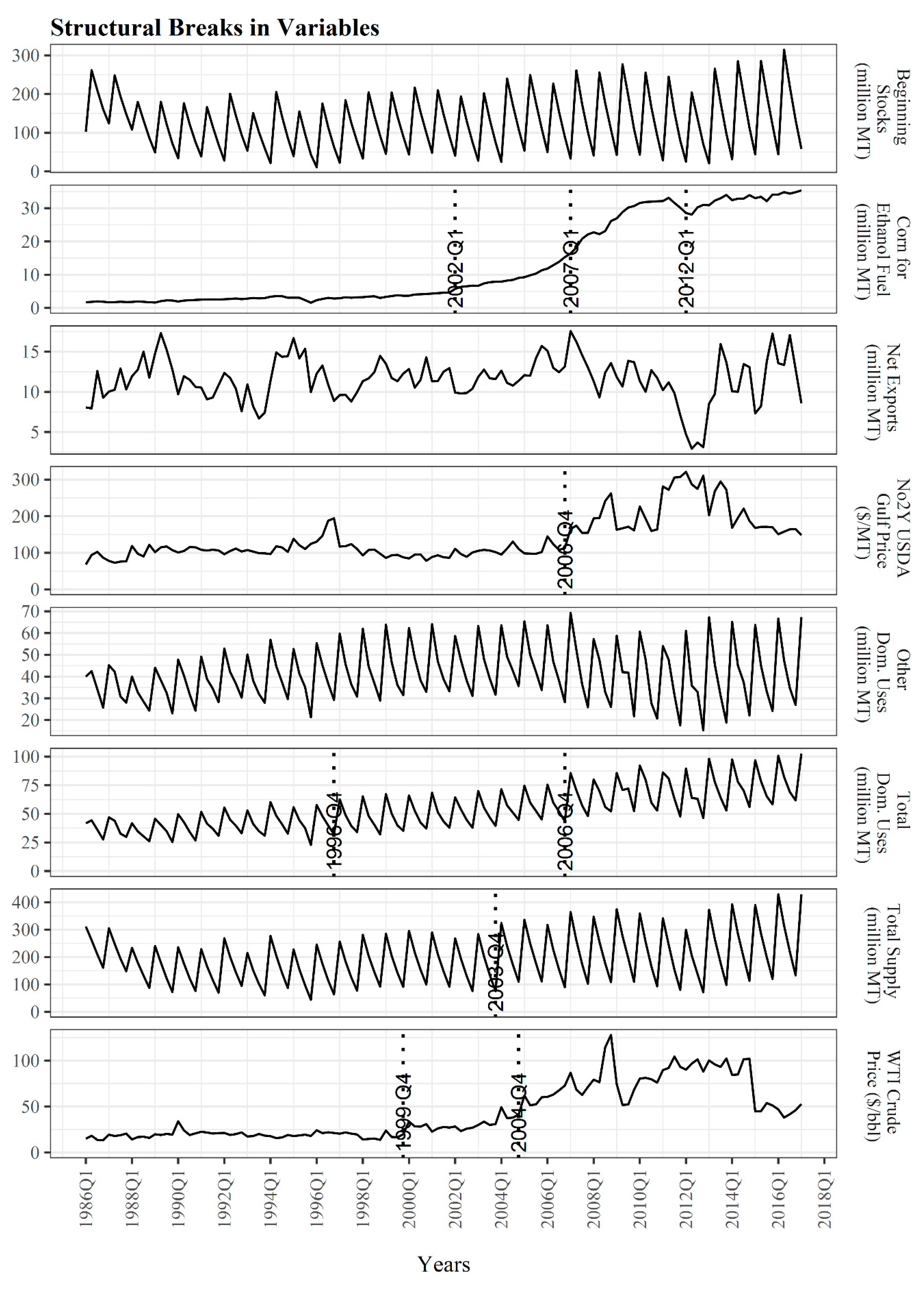
Table 1 shows that nearly all variables have a unit root in levels under the ADF and KPSS tests, particularly when no intercept term is included in the regression. The Zivot-Andrew test shows that the two price variables, as well as corn use for ethanol have a unit root even after accounting for a structural break. In contrast, none of the variables, except for corn ethanol under the KPSS test, has a unit root in first differences. These results imply that most of the variables can be considered non-stationary and integrated of order 1 or I(1). Figure 2 shows that there are structural break-dates in the variables, except beginning stocks, net corn exports and other domestic corn use. The most notable observation is that there are three break-dates in corn use for ethanol, which occur in MY 2002:Q1, MY 2007:Q1 and MY 2012:Q1. There are two break-dates in total domestic corn use (MY 1996:Q4 and MY 2006:Q4) and WTI oil price (MY 1999:Q4 and MY 2004:Q4), and one break-date in total corn supply (MY 2003:Q4) and corn price (MY 2006:Q4).
3.2. Causality Test Results
Given the structural break test results, four structural break variables are included among the deterministic terms in Equation (1) using the flexible Fourier approach [45]. Table 2 presents the Granger-causality (GC) and Instantaneous-causality (IC) test results. The coefficients in Table 2 are estimated with the actual data, using the unrestricted form of Equation (1) with seven lags of each variable. The GC coefficients in Table 2 are averages of the lag coefficients, whereas the IC coefficients are Pearson correlation coefficients of residuals. Although the variables are in logarithms, so that the coefficients are in the form of “causal impact elasticities”, these are not elasticities in the usual sense. In addition, the IC estimates are correlation coefficients, which are related, but different, from regression coefficients. As previously discussed, significance of the GC and IC coefficients are based on bootstrapped critical values and the causality results are applicable in the one-step ahead or next period sense.
Table 2 shows that the corn price and other domestic corn use have significant, negative GC impacts on corn use for ethanol. Corn use for ethanol has significant, negative GC impacts on other domestic corn use and total domestic corn use, as well as a positive impact on total corn supply. There are also significant IC interactions of corn use for ethanol with other domestic corn use, total domestic corn use and total corn supply which are all positive. The only significant GC impact on the corn price is from total corn supply and is negative. The corn price has significant negative GC impacts on corn use for ethanol, as previously highlighted, and a positive GC impact on other domestic corn use. IC interactions of the corn price with other variables are significant and negative for corn use for ethanol, other domestic corn use, total domestic corn use and total corn supply.
Other domestic corn use and total domestic corn use have significant GC impacts on net corn exports, which are positive and negative, respectively, whereas net corn export has a significant, negative GC impact on only total corn supply. IC interactions of net corn exports with other domestic corn use, total domestic corn use, and total corn supply are significant and positive, but negative with the corn price. Total corn supply has significant positive GC impacts on other domestic corn use and total domestic corn use but negative GC impact on the corn price. Similarly, IC interactions of total corn supply with other domestic corn use and total domestic corn use are positive, but negative with the corn price. The GC impact of other domestic corn use on total domestic corn use is significant and negative, whereas their IC interaction is significant and positive.
4. Discussion
4.1. Structural Breaks
All eight variables examined in this paper, except beginning stocks and other domestic corn use, contain at least one structural break in the mean during the MY 1986 to MY 2017 period. The three breaks in corn use for ethanol are in MY 2002, 2007 and 2012. The break-date in the fall of 2002 (MY 2002:Q1) precedes the 2005 RFS1 legislation but falls within the period of public discussions and planning leading up to its enactment. A Blue Ribbon advisory panel of the U.S. Environmental Protection Agency (EPA) called for reductions in MTBE use in 1999 due to its contamination of drinking water [46]. MTBE (methyl tertiary-butyl ether) is a flammable, colorless liquid that dissolves easily in water. It is part of a group of chemicals known as fuel oxygenates that are added to increase gasoline’s oxygen content. California led the way with legislation to eliminate MTBE as an oxygenate in gasoline supplies by December 2002 [47]. In addition, a proposal to eliminate MTBE from all U.S. gasoline was introduced but not passed by the U.S. Senate in 2001 [48]. In response to state bans and potential liability concerns, large fuel producers, such as BP and Exxon, announced plans to eliminate MTBE from their gasoline production by early 2003. Consequently, U.S. ethanol production grew by 21% in 2002 marking a period of double-digit annual growth that lasted until 2010. Thus, the MY 2002:Q1 break in corn use for ethanol identified in this study marks the shift to ethanol initiated by state-level laws on MTBE that by 2005 included more than 20 states [46,47].
The MY 2007:Q1 break in corn use for ethanol occurs in the fall following EPA’s final rule for implementing the RFS1 in April 2007, and just precedes enactment of the RFS2 in December 2007. However, December 2007 was also the official start of the Great Recession of 2008/2009; judged as the second worst in U.S. economic history next to the Great Depression of the 1930s. The data show that corn use for ethanol dipped slightly in MY 2008:Q1, likely because of the recession. The last break-date in corn use for ethanol in MY 2012:Q1 is associated with a sizable dip in corn use for ethanol during the severe drought of 2012. This has been described as the worst U.S. drought to hit the U.S. farm belt since the 1950s [49]. The drought began in 2011 and was most severe in 2012, leading to idled ethanol plants and operations below capacity that impacted U.S. ethanol production trends through 2013 [50].
There are two break-dates in total domestic corn use (MY 1996:Q4 and MY 2006:Q4) and one for total corn supply (MY2003:Q4) in Figure 2. The initial break in domestic corn use occurs as a steep decline in corn prices began in MY 1996:Q4 from nearly USD 200/ton to a low of about USD 75/ton in MY 2000:Q4. The second break in total domestic corn use (MY 2006:Q4) occurs simultaneously with a break in the corn price and precedes by one quarter the break in corn use for ethanol, discussed above, following EPA’s publication of regulations for the RFS2. The MY 2003:Q4 break-date for total corn supply follows the MY 2002:Q1 break in corn use for ethanol and aligns with the rapid expansion of U.S. production to complete the transition from MTBE. The upward shift in total corn supply during this period, visible in Figure 1, is a reasonable response to the increasing corn demand for ethanol production.
Structural breaks also occur in world oil price in MY 1999:Q4 and MY 2004:Q4. These periods align with increases in the oil price. Strong global economic growth during the period from 2003 to 2007 was accompanied by a steady increase in most commodity prices, including oil. Although oil prices started a rapid climb in 2004, corn prices did not break upward until 2006. The single structural break in corn price occurs in the summer of 2007, just preceding the enactment of RFS2.
4.2. Causality
Results show that the corn price has a negative GC impact on corn use for ethanol, but GC impacts in the other direction and IC interactions between the two variables are not significant. In other words, corn ethanol production declines in response to high corn prices, but high corn use for ethanol does not lead to corn price increases. Given these results, corn prices appear to play only a small role in the large increases in corn use for ethanol over the last two decades. However, other domestic corn use has a negative GC impact on corn use for ethanol, indicating that increases (decreases) in other corn uses in previous periods corresponds to lower (higher) corn use for ethanol production in the current period. GC impacts in the other direction, that is of corn use for ethanol production on other domestic corn use, is also significant and negative but is about one order of magnitude smaller. Thus, other domestic corn use is the dominant driver in the lagging relationship with corn use for ethanol. The significant, positive IC results mean that corn use for ethanol, other domestic corn use, and total domestic corn use increase or decrease simultaneously.
Corn use for ethanol also has a positive GC impact on total corn supply, which means that increases in U.S. corn supply over the last two decades were driven in part by corn demand for ethanol production. This is an important finding. Since the shares of biofuels in U.S. petroleum fuels are determined on an annual basis, this finding likely reflects the fact that quarterly variations in corn use for ethanol demand are small as shown in Figure 1. As a result, past quarterly corn use for ethanol is a good predictor of demand, and thus a determinant of total corn supply, in the current quarter. In addition to the GC effects discussed above, IC between corn use for ethanol and total corn supply is also positive, meaning that the two variables also tend to increase or decrease together in the current quarter. These findings follow from the fact that policies to replace MTBE and to develop a Renewable Fuel Standard provide advance notice to markets and impose limited quarter to quarter variations in corn use for ethanol. Therefore, U.S. corn supply, which combines production and stocks, was able to grow with increases in corn demand for ethanol production, using a combination of past information and expected changes. These results are also consistent with the fact that no GC impact from total supply on corn use for ethanol was found in this study, that is, corn use for ethanol in the current period is not driven by total corn supply in previous periods.
Figure 1 clearly shows that corn use for ethanol more than tripled from about 33 million tons in 2004 to nearly 127 million tons from MY 2005 to 2010, whereas other domestic corn use declined by about 17% from about 190 million tons to 156 million tons. Obviously, corn use for ethanol during this period was driven by policy changes, but previous studies have indicated that reductions in other domestic corn use may be traced to the resulting increase in corn use for ethanol demand [51]. The findings in this study mean that changes in other corn use have a stronger impact on corn use for ethanol than the reverse. This may be explained by the fact that livestock producers (representing the largest other domestic user of corn) anticipated policy-driven increases in corn ethanol by reducing their direct use of corn to accommodate corn demand for ethanol, even as total supply increased. This pathway reflects both the contract (planned) nature of corn input into U.S. livestock production and the use of distiller’s dry grains (DDGS) which is a high protein animal feed. In the first instance, the co-production of DDGS means that about 30% of all corn input into corn ethanol production is returned as livestock feed. In the second instance, Hoffman and Baker [52] found that “a metric ton of DDGS can replace, on average, 1.22 metric tons of feed consisting of corn and soybean meal in the United States”. Thus, combined, the quantity and quality of increases in DDGS made up nearly all direct reductions in other domestic corn use between 2005 and 2010.
Complementary explanations for the reduction in other domestic corn use during this period include the stagnation in U.S. cattle output between 2003 and 2007 due to the discovery of mad cow infections in U.S. and Canadian herds. Hanrahan and Becker [53] showed that the ban on U.S. beef exports by its four principal markets, Canada, Mexico, Japan and South Korea, reduced the global share of U.S. beef exports from 18% in 2002 to 3% in 2004, recovering to about 9% in 2007. All cattle and calves inventory, as well as slaughtered cattle, declined in 2004 and did not recover to 2003 levels for several years [54].
There are no significant GC impacts of corn use for ethanol on net corn exports or the corn price, with total corn supply as the only significant GC driver of corn prices. However, total corn supply, net corn exports, other domestic demand and total domestic demand have significant negative IC interactions with the corn price. Thus, total corn supply in previous periods, and corn supply and all corn demand variables in the current period, except corn use for ethanol, jointly drive current period corn prices. The negative impact of total corn supply on corn prices follows from the fact that current period total corn supply is largely fixed, and high corn availability would tend to reduce prices. As previously discussed, total corn supply is essentially equal to beginning stocks during Q2 to Q4 of the MY, and advance projections generally provide accurate estimates of corn production in the first quarter of the marketing year. On the one hand, the lack of any GC impacts from corn demand variables on the corn price mean that these variables are not lagging drivers of corn prices. On the other hand, negative IC interactions with the corn price mean that unexpected increases (decreases) in corn prices would lead to decreases (increases) in corn demand, except corn use for ethanol, in the current period.
The GC results show that net corn exports tend to rise in periods following increases in other domestic corn use, suggesting that, while changes in global corn demand are immediately reflected in domestic demand, effects on U.S. corn exports are lagging. However, the results also imply that net corn exports tend to decrease following periods of higher total domestic corn use, all else equal. This is likely because unexpected jumps in total domestic corn use in one period depletes available supplies in the next period. In contrast, IC results show that high corn exports coincide with high corn use for ethanol production and other domestic corn use in the same period. Total corn supply is a positive GC driver for other domestic corn use and total domestic corn use, but a negative GC driver for the corn price. The positive IC interactions between total corn supply and all demand variables on the one hand, and negative IC between the corn price and all corn demand variable (except corn use for ethanol) on the other, mean that the competition for corn supplies in a given period is mediated by the corn price.
4.3. Summary
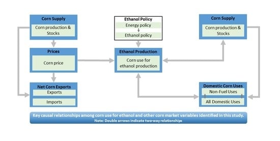
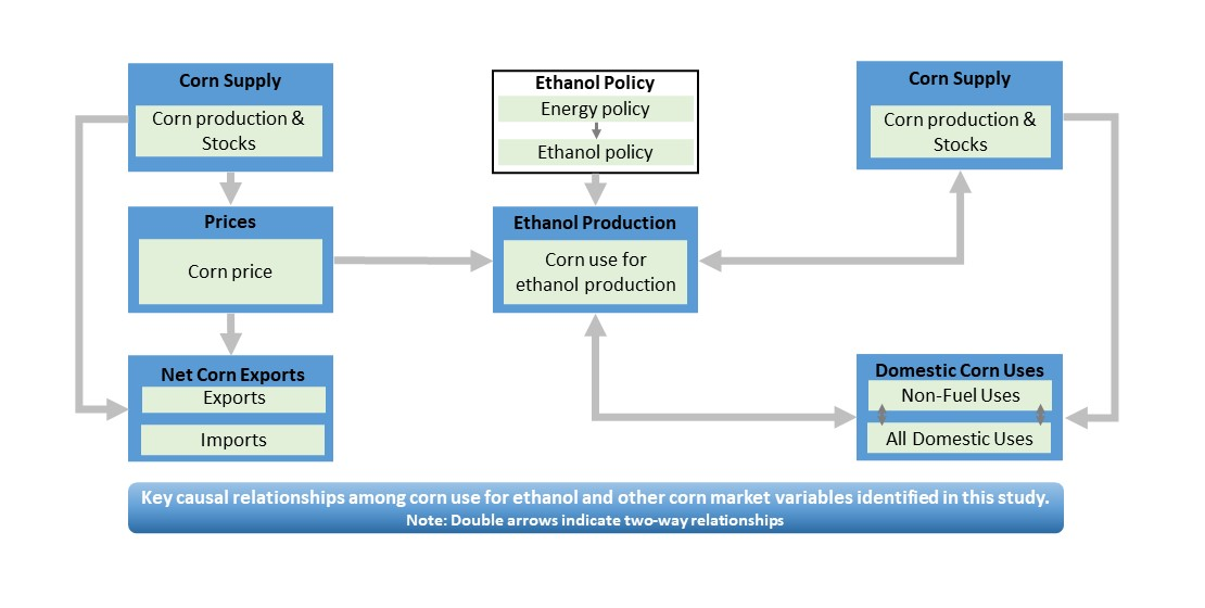
The structural break test results in this study found three break dates in corn use for ethanol that are associated with important events during the period of rapid increases in U.S. ethanol production over the last two decades. These are in MY 2002 marking the period of vigorous public discussion and legislation on oxygenates, MTBE and renewable fuels in U.S. gasoline, MY 2007 during the implementation and expansion of the U.S. renewable fuel standards and MY 2012 during the most severe U.S. drought in the last fifty years. These break dates point to the important role of policy changes in accelerating corn ethanol use in the U.S. Results of the causality analysis are summarized in Figure 3 (panels b and c) and compared with common assumptions (panel a) about the role of corn use for ethanol in corn markets. These causality results contribute a number of insights into the debate about the global agricultural market effects of U.S. biofuel policies. First, it is generally assumed that corn use for ethanol in the U.S. caused increases in corn prices via increased demand for feedstock. This relationship is not confirmed by the empirical data examined in this paper. The GC results did not find that corn use for ethanol is a significant lagging driver of corn prices and there is no significant IC or current period interactions between the two variables. Instead, adjustments and interactions between total corn supply and other domestic corn use appear to account for the large increase in corn use for ethanol production since 2003. Second, enhanced corn ethanol production following the introduction of biofuel policies is thought to affect crop production abroad by limiting corn exports from the U.S. The GC and IC analyses presented here do not support such effects, as there are no significant GC impacts and IC interactions between corn ethanol production and net corn exports. The negative GC impact of total domestic corn use on net corn exports follow directly from the fact that higher than expected total domestic corn use in previous periods generally reduces available supplies in the next period, all else equal. In addition, IC interactions of net corn exports with other domestic corn use and total domestic corn use are positive, so that these three sources of demand for corn increase together in a given period. As would be expected, current period net corn export is also significant and positively related to total corn supply but negatively to the corn price (i.e., higher corn prices tend to diminish exports). Since total corn supply also has strong negative GC impact on and IC interaction with the corn price, these two variables (total supply and price), and not corn use for ethanol, are the key determinants of net corn exports.
5. Conclusions
The findings in this paper point to a different assessment of potential indirect effects of U.S. corn use for ethanol on corn markets than commonly is assumed. First, corn use for ethanol is not found to be a lagging driver of net corn exports, but both increase simultaneously. Second, corn use for ethanol does not have a (lagging or same-period) causal effect on the corn price, which means that it does not affect corn prices. Third, corn use for ethanol is found to be a positive driver of total corn supply, which in turn is a positive driver for all domestic corn uses and exports. Fourth, structural breaks in corn use for ethanol emphasize the policy-driven nature of the U.S. ethanol market over the last two decades, initially driven by state-level legislations/incentives and then by enactment of the national RFS1 in 2005 and RFS2 in 2007. Thus, total corn supply and other domestic corn use appear to be the key pathways of adjustments to the large increase in U.S. corn use for ethanol between 2003 and 2010. No significant role was found for either corn price or net corn exports. The implications of these findings would differ dramatically from common assumptions that link U.S. corn-based ethanol to reduced corn exports, increased global corn prices, and related consequences for global land use change and food markets. As with any empirical analysis, caveats are in order for the work in this paper. The results of this study should be interpreted within the context of the data available for the analysis. Additionally, as discussed previously, the causality results in this paper have a one-step ahead or next period interpretation and do not address potential non-linear causality or other causality concepts. These topics are reserved for future efforts.
Author Contributions
Conceptualization, G.A.O., K.L.K., J.W.A.L.; methodology, G.A.O.; software, G.A.O.; writing—original draft preparation, G.A.O.; writing—review and editing, G.A.O., K.L.K. and J.W.A.L.; visualization, G.A.O.; funding acquisition, K.L.K., G.A.O., J.W.A.L. All authors have read and agreed to the published version of the manuscript.
Funding
The efforts of Gbadebo Oladosu and Keith Kline were funded was funded by the U.S. Department of Energy, Bioenergy Technology Office. The contribution of J.W.A.L was funded under International Energy Agency (IEA) Bioenergy Technology Collaboration Programme, Task 43.
Institutional Review Board Statement
Not Applicable.
Informed Consent Statement
Not Applicable.
Data Availability Statement
All data used in this paper are from public sources.
Acknowledgments
The authors would like to acknowledge and express their appreciation to the U.S. Department of Energy, Bioenergy Technology Office. Thanks to two anonymous reviewers who provided valuable comments on the manuscript. We also thank Rocio Uria-Martinez for her review of the final pre-submission version of the manuscript, as well as collaborators under the IEA Bioenergy Task 43 for their support (Mudit. Chordia, Miguel Brandão, Annette Cowie).
Conflicts of Interest
The authors declare no conflict of interest.
Copyright Notice
This manuscript has been authored by UT-Battelle, LLC under Contract No. DE-AC0500OR22725 with the U.S. Department of Energy. The United States Government retains and the publisher, by accepting the article for publication, acknowledges that the United States Government retains a non-exclusive, paid-up, irrevocable, world-wide license to publish or reproduce the published form of this manuscript, or allow others to do so, for United States Government purposes. The Department of Energy will provide public access to these results of federally sponsored research in accordance with the DOE Public Access Plan (http://energy.gov/downloads/doe-public-accessplan).
References
- Searchinger, T.; Heimlich, R.; Houghton, R.A.; Dong, F.; Elobeid, A.; Fabiosa, J.; Tokgoz, S.; Hayes, D.; Yu, T.H. Use of US Croplands for Biofuels Increases Greenhouse Gases through Emissions from Land-Use Change. Science 2008, 319, 1238–1240. [Google Scholar] [CrossRef] [PubMed]
- Condon, N.; Klemick, H.; Wolverton, A. Impacts of Ethanol Policy on Corn Prices: A Review and Meta-Analysis of Recent Evidence. Food Policy 2015, 51, 63–73. [Google Scholar] [CrossRef]
- Kline, K.L.; Msangi, S.; Dale, V.H.; Woods, J.; Souza, G.M.; Osseweijer, P.; Clancy, J.S.; Hilbert, J.A.; Johnson, F.X.; McDonnell, P.C.; et al. Reconciling Food Security and Bioenergy: Priorities for Action. Gcb Bioenergy 2017, 9, 557–576. [Google Scholar] [CrossRef] [Green Version]
- Oladosu, G.; Msangi, S. Biofuel-Food Market Interactions: A Review of Modeling Approaches and Findings. Agriculture 2013, 3, 53–71. [Google Scholar] [CrossRef] [Green Version]
- Persson, U.M. The Impact of Biofuel Demand on Agricultural Commodity Prices: A Systematic Review. Wiley Interdiscip. Rev. Energy Environ. 2015, 4, 410–428. [Google Scholar] [CrossRef]
- Wicke, B.; Verweij, P.; Meijl, H.; Vuuren, D.P.; Faaij, A.P. Indirect Land Use Change: Review of Existing Models and Strategies for Mitigation. Biofuels 2012, 3, 87–100. [Google Scholar] [CrossRef]
- Dunn, J.B.; Merz, D.; Copenhaver, K.L.; Mueller, S. Measured Extent of Agricultural Expansion Depends on Analysis Technique. Biofuels Bioprod. Biorefining 2017, 11, 247–257. [Google Scholar] [CrossRef] [Green Version]
- Malins, C.; Plevin, R.; Edwards, R. How Robust Are Reductions in Modeled Estimates from GTAP-BIO of the Indirect Land Use Change Induced by Conventional Biofuels? J. Clean. Prod. 2020, 258, 120716. [Google Scholar] [CrossRef]
- Efroymson, R.A.; Kline, K.L.; Angelsen, A.; Verburg, P.H.; Dale, V.H.; Langeveld, J.W.; McBride, A. A Causal Analysis Framework for Land-Use Change and the Potential Role of Bioenergy Policy. Land Use Policy 2016, 59, 516–527. [Google Scholar] [CrossRef] [Green Version]
- Zhang, Z.; Luanne, L.; Escalante, C.; Wetzstein, M. Food versus Fuel: What Do Prices Tell Us? Energy Policy 2008, 38, 445–451. [Google Scholar] [CrossRef]
- Cha, K.S.; Bae, J.H. Dynamic Impacts of High Oil Prices on the Bioethanol and Feedstock Markets. Energy Policy 2011, 39, 753–760. [Google Scholar] [CrossRef]
- Qui, C.; Colson, G.; Escalante, C.; Wetztein, M. Considering Macroeconomic Indicators in the Food before Fuel Nexus. Energy Econ. 2012, 34, 2021–2028. [Google Scholar]
- Nazlioglu, S.; Soytas, U. Oil Price, Agricultural Commodity Prices, and the Dollar: A Panel Cointegration and Causality Analysis. Energy Econ. 2012, 34, 1098–1104. [Google Scholar] [CrossRef]
- Natanelov, V.; Alam, M.J.; McKenzie, A.M.; Huylenbroeck, G.V. Is There Co-Movement of Agricultural Commodities Futures Prices and Crude Oil? Energy Policy 2011, 39, 4971–4984. [Google Scholar] [CrossRef] [Green Version]
- Ciaian, P. Interdependencies in the Energy–Bioenergy–Food Price Systems: A Cointegration Analysis. Resour. Energy Econ. 2011, 33, 326–348. [Google Scholar] [CrossRef]
- Nazlioglu, S. World Oil and Agricultural Commodity Prices: Evidence from Nonlinear Causality. Energy Policy 2011, 39, 2935–2943. [Google Scholar] [CrossRef]
- Harri, A.; Nally, L.; Hudson, D. The Relationship between Oil, Exchange Rates, and Commodity Prices. J Agric. Appl. Econ. 2009, 41, 501–510. [Google Scholar] [CrossRef] [Green Version]
- Katrakilidis, C.; Sidiropoulos, M.; Tabakis, N. An Empirical Investigation of the Price Linkages between Oil, Biofuels and Selected Agricultural Commodities. Procedia Econ. Financ. 2015, 33, 313–320. [Google Scholar] [CrossRef] [Green Version]
- Papiez, M. A dynamic analysis of causality between prices of corn, crude oil and ethanol. In Proceedings of the 32nd International Conference on Mathematical Methods in Economics, Olomouc, Czech Republic, 10–12 September 2014. [Google Scholar]
- Rezitis, A.N. The Relationship between Agricultural Commodity Prices, Crude Oil Prices and US Dollar Exchange Rates: A Panel VAR Approach and Causality Analysis. Int. Rev. Appl. Econ. 2015, 29, 403–434. [Google Scholar] [CrossRef]
- Filip, O.; Janda, K.; Kristoufek, L.; Zilberman, D. Food versus Fuel: An Updated and Expanded Evidence. Energy Econ. 2017, 82, 152–166. [Google Scholar] [CrossRef] [Green Version]
- Chen, B.; Saghaian, S. Market Integration and Price Transmission in the World Rice Export Markets. J. Agric. Resour. Econ. 2016, 41, 444–457. [Google Scholar]
- Taghizadeh-Hesary, F.; Rasoulinezhad, E.; Yoshino, N. Trade Linkages and Transmission of Oil Price Fluctuations in a Model Incorporating Monetary Variables. Energy Policy. 2019, 133, 110872. [Google Scholar] [CrossRef]
- Roman, M.; Górecka, A.; Domagała, J. The Linkages between Crude Oil and Food Prices. Energies 2020, 13, 6545. [Google Scholar] [CrossRef]
- Vo, D.H.; Vu, T.N.; McAleer, M. Modeling the Relationship between Crude Oil and Agricultural Commodity Prices. Energies 2019, 12, 1344. [Google Scholar] [CrossRef] [Green Version]
- Eigenbrod, F.; Beckmann, M.; Dunnett, S.; Graham, L.; Holland, R.A.; Meyfroidt, P.; Seppelt, R.; Song, X.-P.; Spake, R.; Václavík, T.; et al. Identifying Agricultural Frontiers for Modeling Global Cropland Expansion. One Earth 2020, 3, 504–514. [Google Scholar] [CrossRef]
- Granger, C.W. Investigating Causal Relations by Econometric Models and Cross-Spectral Methods. Econom. J. Econom. Soc. 1969, 1, 424–438. [Google Scholar] [CrossRef]
- Seth, A.K.; Barrett, A.B.; Barnett, L. Granger Causality Analysis in Neuroscience and Neuroimaging. J. Neurosci. 2015, 35, 3293–3297. [Google Scholar] [CrossRef] [PubMed]
- ERS. Feed Grains Database; Economic Research Service, US Department of Agriculture: Washington, DC, USA, 2018. Available online: https://www.ers.usda.gov/data-products/feed-grains-database/ (accessed on 24 February 2021).
- EIA. Cushing, OK WTI Spot Price FOB; Energy Information Administration, US Department of Energy: Washington, DC, USA, 2018. Available online: https://www.eia.gov/dnav/pet/hist/RWTCD.htm (accessed on 24 February 2021).
- Bastianin, A.; Galeotti, M.; Manera, M. Causality and Predictability in Distribution: The Ethanol–Food Price Relation Revisited. Energy Econ. 2014, 42, 152–160. [Google Scholar] [CrossRef]
- Gilbert, C.L. How to Understand High Food Prices. J. Agric. Econ. 2010, 61, 398–425. [Google Scholar] [CrossRef]
- Saghaian, S.H. The Impact of the Oil Sector on Commodity Prices: Correlation or Causation? J. Agric. Appl. Econ. 2010, 42, 477–485. [Google Scholar] [CrossRef] [Green Version]
- Tiwari, A.K.; Ludwig, A. Short-and Long-Run Rolling Causality Techniques and Optimal Window-Wise Lag Selection: An Application to the Export-Led Growth Hypothesis. J. Appl. Stat. 2015, 42, 662–675. [Google Scholar] [CrossRef]
- Nyakabawo, W.; Miller, S.M.; Balcilar, M.; Das, S.; Gupta, R. Temporal Causality between House Prices and Output in the US: A Bootstrap Rolling-Window Approach. N. Am. J. Econ. Financ. 2015, 33, 55–73. [Google Scholar] [CrossRef] [Green Version]
- Balcilar, M.; Ozdemir, Z.A.; Arslanturk, Y. Economic Growth and Energy Consumption Causal Nexus Viewed through a Bootstrap Rolling Window. Energy Econ. 2010, 32, 1398–1410. [Google Scholar] [CrossRef]
- Toda, H.Y.; Yamamoto, T. Statistical Inference in Vector Autoregressions with Possibly Integrated Processes. J. Econom. 1995, 66, 225–250. [Google Scholar] [CrossRef]
- Lütkepohl, H. New Introduction to Multiple Time Series Analysis; Springer Science & Business Media: Berlin/Heidelberg, Germany, 2005. [Google Scholar]
- Hansen, B.E. The New Econometrics of Structural Change: Dating Breaks in US Labour Productivity. J. Econ. Perspect. 2001, 15, 117–128. [Google Scholar] [CrossRef] [Green Version]
- Glynn, J.; Perera, N. Unit Root Tests and Structural Breaks: A Survey with Applications Contrastes de raíces unitarias y cambios estructurales: Un estudio con aplicaciones. Rev. Métod. Cuantitativos Para Econ. Empresa J. Quant. Methods Econ. Bus. Adm. 2007, 3, 63–79. [Google Scholar]
- Kwiatkowski, D.; Phillips, P.C.; Schmidt, P.; Shin, Y. Testing the Null Hypothesis of Stationarity against the Alternative of a Unit Root: How Sure Are We That Economic Time Series Have a Unit Root? J. Econom. 1992, 54, 159–178. [Google Scholar] [CrossRef]
- Zivot, E.; Andrews, D.W. Further Evidence on the Great Crash, the Oil-Price Shock, and the Unit-Root Hypothesis. J. Bus. Econ. Stat. 2002, 20, 25–44. [Google Scholar] [CrossRef]
- Bai, J.; Perron, P. Computation and Analysis of Multiple Structural Change Models. J. Appl. Econom. 2003, 18, 1–22. [Google Scholar] [CrossRef] [Green Version]
- Hafner, C.M.; Herwartz, H. Testing for Linear Vector Autoregressive Dynamics under Multivariate Generalized Autoregressive Heteroskedasticity. Stat. Neerl. 2009, 63, 294–323. [Google Scholar] [CrossRef]
- Enders, W.; Jones, P. Grain Prices, Oil Prices, and Multiple Smooth Breaks in a VAR. Stud. Nonlinear Dyn. Econom. 2016, 20, 399–419. [Google Scholar] [CrossRef]
- McCarthy, J.E.; Tiemann, M. Tiemann MTBE in Gasoline: Clean Air and Drinking Water Issues. In Congressional Research Service Reports; Congressional Research Service, The Library of Congress: Washington, DC, USA, 2006; p. 26, 98-290 ENR. [Google Scholar]
- Anderson, S.T.; Elzinga, A. A Ban on One Is a Boon for the Other: Strict Gasoline Content Rules and Implicit Ethanol Blending Mandates. J. Environ. Econ. Manag. 2014, 67, 258–273. [Google Scholar] [CrossRef]
- US Senate. S.265 - MTBE Elimination Act—107th Congress (2001-2002); Government Printing Office: Washington, DC, USA, 2001. Available online: https://www.congress.gov/107/bills/s265/BILLS-107s265is.pdf (accessed on 24 February 2021).
- Rippey, B.R. The US Drought of 2012. Weather Clim. Extrem. 2015, 10, 57–64. [Google Scholar] [CrossRef] [Green Version]
- RFA. Monthly Ethanol Supply and Demand Data; Renewable Fuel Association: Ellisville, MI, USA, 2020; Available online: https://ethanolrfa.org/statistics/weekly-monthly-ethanol-supply-demand/ (accessed on 24 February 2021).
- Oladosu, G.; Kline, K.; Uria-Martinez, R.; Eaton, L. Sources of Corn for Ethanol Production in the United States: A Decomposition Analysis of the Empirical Data. Biofuels Bioprod. Biorefining 2011, 5, 640–653. [Google Scholar] [CrossRef]
- Hoffman, L.A.; Baker, A.J. Estimating the Substitution of Distillers’ Grains for Corn and Soybean Meal in the US Feed Complex; US Department of Agriculture: Washington, DC, USA, 2011. [Google Scholar]
- Hanrahan, C.E.; Becker, G.S. Mad Cow Disease and US Beef Trade; Congressional Research Service, Library of Congress: Washington, DC, USA, 2006. [Google Scholar]
- USDA. Cattle & Beef Statistics; US Department of Agriculture: Washington, DC, USA, 2020. Available online: https://www.ers.usda.gov/topics/animal-products/cattle-beef/statistics-information.aspx (accessed on 24 February 2021).
Figure 1.
U.S. quarterly corn market and other data by corn marketing year. Note different scales on charts. The price of yellow corn as reported at the key export port (No2Y Corn Gulf) represents global corn prices for this analysis.
Figure 1.
U.S. quarterly corn market and other data by corn marketing year. Note different scales on charts. The price of yellow corn as reported at the key export port (No2Y Corn Gulf) represents global corn prices for this analysis.

Figure 2.
Structural break-dates (vertical lines) in mean of U.S. corn market data.

Figure 3.
Interactions among corn market variables based on common assumptions (panel a) versus Granger (panel b) and Instantaneous (panel c) causality results in the current study. Relationships among corn use for ethanol and other variables are emphasized by dashed lines Note that Other and Total domestic corn use are combined in this figure for clarity.


Table 1.
Unit root test results for U.S. MY quarterly data (* indicates unit root at 5% level).
| ADF Test | KPSS Test | Zivot-Andrew Test | |||||||
|---|---|---|---|---|---|---|---|---|---|
| Variables | None | Drift | Trend | Drift | Trend | Drift | Trend | Both | |
| Beginning Stocks | Level | −3.36 | −12.36 | −12.86 | 0.34 | 0.13 | −15.64 | −15.89 | −15.81 |
| 1st Diff. | −15.11 | −15.04 | −14.98 | 0.01 | 0.01 | −15.27 | −15.27 | −15.38 | |
| Total Supply | Level | −2.35 | −10.89 | −13.28 | 1.11 * | 0.14 | −15.47 | −15.75 | −15.68 |
| 1st Diff. | −14.97 | −14.91 | −14.86 | 0.03 | 0.01 | −14.88 | −14.88 | −14.97 | |
| Price (No2 Y Gulf) | Level | −0.66 * | −2.29 * | −2.94 * | 3.35 * | 0.50 * | −4.32 * | −3.29 * | −5.93 |
| 1st Diff. | −11.55 | −11.51 | −11.47 | 0.04 | 0.04 | −12.29 | −11.81 | −12.28 | |
| Net Corn Exports | Level | −0.98 * | −5.41 | −5.40 | 0.11 | 0.10 | −5.78 | −5.46 | −6.49 |
| 1st Diff. | −10.65 | −10.60 | −10.56 | 0.03 | 0.01 | −10.77 | −10.67 | −11.24 | |
| Corn for Ethanol Fuel | Level | 2.71 * | 1.04 * | −1.55 * | 5.50 * | 1.35 * | −4.62 * | −2.23 * | −2.75 * |
| 1st Diff. | −4.63 | −5.23 | −5.50 | 0.81 * | 0.21 * | −6.73 | −6.08 | −6.68 | |
| Other Domestic Uses | Level | −1.58 * | −12.49 | −13.17 | 0.47 * | 0.19 * | −16.19 | −15.42 | −16.27 |
| 1st Diff. | −14.55 | −14.49 | −14.43 | 0.01 | 0.01 | −14.43 | −14.43 | −14.50 | |
| Total Domestic Use | Level | −0.86 * | −4.72 | −14.27 | 4.72 * | 0.13 | −15.99 | −15.61 | −15.96 |
| 1st Diff. | −14.54 | −14.50 | −14.44 | 0.02 | 0.01 | −14.44 | −14.44 | −14.50 | |
| WTI Crude Price | Level | −0.89 * | −2.05 * | −3.22 * | 4.58 * | 0.51 * | −4.98 | −4.21 * | −4.68 * |
| 1st Diff. | −11.44 | −11.41 | −11.38 | 0.04 | 0.04 | −12.03 | −11.66 | −13.09 | |
| Critical Values | 1% | −2.58 | −3.46 | −3.99 | 0.74 | 0.22 | −5.34 | −4.93 | −5.57 |
| 5% | −1.95 | −2.88 | −3.43 | 0.46 | 0.15 | −4.80 | −4.42 | −5.08 | |
| 10% | −1.62 | −2.57 | −3.13 | 0.35 | 0.12 | −4.58 | −4.11 | −4.82 | |
Table 2.
Granger and instantaneous causality test results (Significance: *** = 1%, ** = 5%, * = 10%).
Table 2.
Granger and instantaneous causality test results (Significance: *** = 1%, ** = 5%, * = 10%).
| Impact | Driver | Granger | Instantaneous |
|---|---|---|---|
| Corn for Ethanol | Net Exports | −0.02 | 0.04 |
| No2Y Corn Gulf Price | −0.05 * | −0.01 | |
| Other Dom. Uses | −0.24 * | 0.28 ** | |
| Total Dom. Uses | −0.02 | 0.41 *** | |
| Total Supply | 0.04 | 0.23 * | |
| Net Exports | Corn for Ethanol | 0.11 | 0.04 |
| No2Y Corn Gulf Price | −0.12 | −0.35 *** | |
| Other Dom. Uses | 0.47 ** | 0.34 *** | |
| Total Dom. Uses | −1.09 ** | 0.37 *** | |
| Total Supply | 0.09 | 0.22 ** | |
| No2Y Corn Gulf Price | Corn for Ethanol | −0.08 | −0.01 |
| Net Exports | 0.03 | −0.35 *** | |
| Other Dom. Uses | 0.22 | −0.25 *** | |
| Total Dom. Uses | 0.13 | −0.37 *** | |
| Total Supply | −0.24 * | −0.17 * | |
| Other Dom. Uses | Corn for Ethanol | −0.04 ** | 0.28 ** |
| Net Exports | 0.00 | 0.34 *** | |
| No2Y Corn Gulf Price | 0.02 * | −0.25 *** | |
| Total Dom. Uses | 0.08 | 0.91 *** | |
| Total Supply | 0.28 ** | 0.49 *** | |
| Total Dom. Uses | Corn for Ethanol | −0.03 ** | 0.41 *** |
| Net Exports | 0.00 | 0.37 *** | |
| No2Y Corn Gulf Price | 0.00 | −0.37 *** | |
| Other Dom. Uses | −0.39 ** | 0.91 *** | |
| Total Supply | 0.21 * | 0.60 *** | |
| Total Supply | Corn for Ethanol | 0.02 *** | 0.23 * |
| Net Exports | −0.01 ** | 0.22 ** | |
| No2Y Corn Gulf Price | 0.03 | −0.17 * | |
| Other Dom. Uses | −0.38 * | 0.49 *** | |
| Total Dom. Uses | −0.06 *** | 0.60 *** |
Note: The Granger coefficients are averages of the p-lag (p = 7) coefficients for each causal driver, and the IC coefficients are Pearson correlation coefficients. Significance levels are based on bootstrapped critical values and the causality results are applicable in the one-step ahead or next period sense.
Publisher’s Note: MDPI stays neutral with regard to jurisdictional claims in published maps and institutional affiliations. |
© 2021 by the authors. Licensee MDPI, Basel, Switzerland. This article is an open access article distributed under the terms and conditions of the Creative Commons Attribution (CC BY) license (http://creativecommons.org/licenses/by/4.0/).
Share and Cite
MDPI and ACS Style
Oladosu, G.A.; Kline, K.L.; Langeveld, J.W.A. Structural Break and Causal Analyses of U.S. Corn Use for Ethanol and Other Corn Market Variables. Agriculture 2021, 11, 267. https://0-doi-org.brum.beds.ac.uk/10.3390/agriculture11030267
AMA Style
Oladosu GA, Kline KL, Langeveld JWA. Structural Break and Causal Analyses of U.S. Corn Use for Ethanol and Other Corn Market Variables. Agriculture. 2021; 11(3):267. https://0-doi-org.brum.beds.ac.uk/10.3390/agriculture11030267
Chicago/Turabian StyleOladosu, Gbadebo A., Keith L. Kline, and Johannes W. A. Langeveld. 2021. "Structural Break and Causal Analyses of U.S. Corn Use for Ethanol and Other Corn Market Variables" Agriculture 11, no. 3: 267. https://0-doi-org.brum.beds.ac.uk/10.3390/agriculture11030267
Note that from the first issue of 2016, this journal uses article numbers instead of page numbers. See further details here.