Drivers of Productivity Change in the Italian Tomato Food Value Chain

Abstract

This study evaluated productivity dynamics and identified sources of productivity growth in Italian tomato production and processing. We used a stochastic frontier input distance function with four error components—heterogeneity, statistical noise, persistent and transient inefficiency—and a four-step estimation procedure with a system generalized method of moments (GMM) estimator in the first step to address the endogeneity problem. The results reveal significant differences in the productivity and efficiency of tomato production and processing. Moreover, there are considerable differences among the different sizes of tomato producers, with the main variations observed for scale efficiency. While tomato processors operate at an optimal production size, tomato producers are characterized by considerable economies of scale, especially small producers. These results thus suggest that there is significant opportunity for technical efficiency improvements at both stages of the value chain. Finally, due to improvements made to scale efficiency, extensive productivity growth was observed for the group of small tomato producers.

1. Introduction

Tomatoes represent one of the most important crops worldwide [1,2,3,4], and tomato production has increased by 300% over the last four decades [5]. Being rich in antioxidants, tomatoes have been recognized to have positive health benefits [3,6]. Today the market is oriented to two types of cultivated tomato: those used for fresh consumption and those used for industrial processing that are usually grown in field conditions [3]. European tomato production, according to FAOSTAT (Statistics Division of the Food and Agriculture Organization of the United Nations) data [7], steadily represents around 13% of global tomato production. In 2020, almost 17 million tons of tomatoes were harvested in the European Union [8,9]. The most important EU producer was Italy, contributing 38% to the total EU production. Italy’s total national production in 2020 was 6.248 million tons, cultivated on a surface of 100,000 hectares (ha) [8]. Almost 75% of Italian tomato production is oriented towards processing and the rest for fresh consumption [8]. Moreover, Italian tomato production is highly geographically concentrated, with two major production regions: Emilia-Romagna in the north and Apulia in the south. These two regions alone produced 35% and 32%, respectively, of the country’s processing tomatoes in 2018 [4].

The tomato processing sector is the basis of the Italian food economy. Italy, with a 13% share in global tomato processing [10], is one of the world’s leading producers of processing tomatoes, being the largest in the Mediterranean region and the third largest worldwide after California and China [4,6,11,12]. Among Italy’s processed tomato production, mashed tomatoes represent about 50% of packaged tomato volume [12]. The processed tomato sector is also important for Italy’s international trade [9] since 60% of Italian production is exported to foreign markets [6]. With 747,000 tons of exported pasta tomatoes and 1.432 million tons of canned tomatoes, Italy is the leading exporter of tomato products [7].

In the last decade, the entire Italian tomato processing supply chain has experienced profound restructuring triggered by the reform of the Common Market Organisation, which has also been accompanied by increasingly fierce price competition in foreign markets [13]. To cope with aggressive trade policies focused on low production costs, Italian tomato producers and processors need to improve their productivity and efficiency.

Productivity is commonly defined as the ability of production factors to produce outputs [14] and is measured as the ratio of a volume measure of output to a volume measure of input use [15]. Since it reflects the overall efficiency of production through its capacity to transform inputs into outputs (both in terms of quantity and quality), it is often used as an indicator of competitiveness [16]. Productivity can be measured at different levels, as a partial measure or as a multifactor measure. The most comprehensive measure is total factor productivity (TFP), which refers to the ratio of aggregated output to a composite index of all inputs [17].

Productivity and, consequently, competitiveness can be increased in different ways. One way to increase competitiveness is to reduce average costs per unit of output by capturing economies of scale [18]. Cost advantages can also be obtained through capital-intensive technological development, in other words, through innovations. Generally, technological change, which refers to changes in production technologies either via improving the existing methods of input use (disembodied technological change) or through changes to input quality (embodied technological change) [19], increases productivity and reduces the input costs per unit of product [20]. Finally, productivity can also be increased by reducing technical ineffectiveness of the product transformation process.

Technical efficiency was originally defined by Koopmans in 1951 [21] as a situation whereby an increase in any output is impossible without a reduction in at least one other output or an increase in at least one input (output-oriented technical efficiency) and whereby a reduction in any input requires an increase in at least one other input or a reduction in at least one output (input-oriented technical efficiency). Measuring technical efficiency presupposes the existence of a production boundary that reflects an efficient input–output subset. The formulation of such a theoretical framework allows us to consider technical efficiency as the distance from the point of the current input–output combination to the boundary [22]. Empirically speaking, technical efficiency represents the deviation of productive performance from best practices. This deviation is usually assigned to either differential management capabilities or to the external environment in which a producer operates [23]. Deeper insights into overall technical inefficiency is provided when it is broken down into transient and persistent parts. The transient component of technical inefficiency relates to non-systematic management problems, shocks associated with new production technologies and changes in human capital [24]. The persistent component of technical inefficiency is related to structural problems in the organization of the production process or to systematic shortfalls in managerial capabilities [25].

Previous research has deeply analyzed the productivity and efficiency of agriculture and food processing (focusing on tomato production, see, e.g., [26,27,28,29,30,31,32,33,34,35,36,37,38,39,40]). Employing different analytical approaches, researchers in this area have used total factor productivity or partial (particularly labor) productivity measures, as well as data envelopment analysis (DEA) and stochastic frontier analysis (SFA), among others. As examples, we can highlight Badenetti et al. [26] who investigated the technical efficiency of tomato production in Italy using SFA; Khan and Ali [27] who employed SFA to investigate the time-invariant technical efficiency of tomato producers in Pakistan; Ogunniyi and Oladejo [28] who estimated the technical efficiency for tomato farmers in the Oyo State of Nigeria using DEA; Tabe-Ojong and Molua [29] who estimated the time-invariant technical efficiency of small-scale tomato production in Cameroon employing SFA and Adenuga et al. [33] who assessed the time-varying technical efficiency of dry season tomato production in Nigeria using SFA. A common feature of these studies is an overall focus on the one stage of production along the agri-food chain (e.g., production or processing) with a predominance of production-level analysis. Moreover, these studies usually do not take into account both components (transient and persistent) of technical efficiency, as they do not employ the most advanced approaches to technical efficiency analysis that emphasize the importance of considering latent heterogeneity in generating an unbiased estimate of time-invariant technical inefficiency, as well as the possibility of efficiency improvements [41] that represent a source of productivity growth [30]. However, unbiased estimates and comprehensive information are necessary for policymakers to formulate relevant policy measures that support the competitiveness of the agri-food value chain in an effective, efficient and economical way [42,43].

In this study, we aimed to evaluate technical efficiency and productivity dynamics and to identify sources that induce productivity change across the tomato vertical chain. In particular, the study addresses the following: the impacts and dynamics of the overall technical efficiency at individual stages along Italy’s tomato supply chain, the dynamics of productivity and its drivers at individual stages of the tomato supply chain and the diffusion effects and the identification of sources that induce productivity changes across the tomato supply chain.

This study contributes to the literature in several ways. First, to the best of our knowledge, despite the numerous previous productivity and efficiency studies, there is a considerable gap of comprehensive research of the whole tomato value chain that identifies the factors that determine successful growth while also capturing the simultaneous relations within the supply chain. Second, it investigated the basic prerequisites of competitiveness, that is technical and scale efficiency and technological change, thus employing new methodological advances in productivity and efficiency analysis.

The rest of this paper is structured as follows: Section 2 introduces the datasets, economic model and estimation strategy, followed by Section 3, which presents the results of this study. Section 4 summarizes and discusses our findings and provides concluding remarks.

2. Materials and Methods

This study used two unbalanced panel datasets of Italian tomato producing and processing companies. The first dataset was drawn from the Farm Accountancy Data Network (FADN) database, which provides harmonized microeconomic data of agricultural holdings. The following variables for tomato producers were obtained from this database: tomato output (yC), defined as the tomato production in tonnes; other farm output (yAOC), measured as the difference between the value of total crop output minus value of tomato output plus value of total livestock and other output; capital (xC), represented by the sum of contract work and capital depreciation; land (xL), expressed in hectares of farm Utilized Agricultural Area (UAA); labor (xW), measured in annual work units (AWU) and materials (xM), defined as total intermediate consumption. Monetary variables were deflated using the price indices from the EUROSTAT database (2010 = 100; apri_pi10). More specifically, index for crop output and agricultural goods output were used to deflate the output of other crops and farm output variables. The price index for machinery and other equipment was used to adjust the capital inputs, and the price index for goods and services currently consumed in agriculture was employed to deflate materials.

Not all of the tomato producers in the FADN database have complete information; thus, observations for those companies with negative and zero values of the variables of interest were excluded from our dataset. Moreover, to ensure a sufficient number of lagged instruments for the econometric model estimation, companies with less than five consecutive years of observations were excluded as well. These procedures constrained the panel dataset to 680 observations of 149 tomato producers in the analyzed period of 2004–2017.

The second dataset represents the tomato processing industry and was obtained from the Amadeus database collected by Bureau van Dijk, a Moody’s Analytics company. For this dataset, desk research was used to identify and select tomato processors from the processors in the NACE-C10.3 category (processing and preserving of fruit and vegetables). In other words, the panel dataset used in our analysis contains companies whose main activity is tomato food processing according to the NACE classification and further investigation of each company’s website. After the removal of companies with incomplete information and fewer than five observations to comply with the requirements of the econometric model estimator, our panel dataset, representing the period from 2006 to 2018, contains 93 companies processing only tomatoes or mainly tomatoes.

At the processing level, we used the following variables: output (y), represented by operating revenue (turnover) and changes in a company’s stock deflated by the sectoral index of food processing prices (NACE 10.3; 2010 = 100); labor (xW), expressed by the cost of employees deflated by the index of producer prices in the industry (2010 = 100); capital (xC), expressed by the book value of fixed assets deflated by the index of producer prices in the industry (2010 = 100) and materials (xM), represented by the total cost of materials and energy deflated by the index of producer prices in the industry (2010 = 100). The source of the price indexes was the EUROSTAT database (sts_ind_pric).

Table 1. Structure of the datasets. Source: FADN and Amadeus.

Tomato Producers
Data	Small	Medium	Large	Total
I	45	54	50	149
NO	223	226	231	680
Tomato processors
Data	Small and medium		Large processors	Total
I	47		46	93
NO	366		380	746

Note: I denotes the number of companies; NO denotes the number of observations.

presents the structure of the data subsets according to size. At the agricultural level, the group of small tomato producers represents one-third of companies in the sample with the lowest economic size, defined according to Regulation (EC) No. 1242/2008; the group of large producers represents one-third of our sample with the highest economic size, and the rest is the group of medium tomato producers. At the processing level, the group of large tomato processors contains companies that employ at least 150 employees and/or have total assets of at least EUR 20 million and/or have operating revenues of at least EUR 10 million. Companies that do not meet these criteria were classified as small and medium-sized.

This analysis applies the micro-level dynamic framework of the total factor productivity (TFP) defined as a ratio that relates the aggregation of all outputs to the aggregation of all inputs [14]. To analyze productivity dynamics and its drivers, we employed the Törnqvist–Theil index (TTI), which is defined as the ratio of the revenue-share weighted geometric mean of individual outputs to the cost share weighted geometric mean of individual inputs [44]. The logarithmic form of TTI between period t and t−1 for the i-th producer can be expressed as [45]:

$$\ln \left(\frac{TF{P}_{it}}{TF{P}_{i\left(t-1\right)}}\right)=\frac{1}{2}{\displaystyle \sum }_{m=1}^M\left(R_{m,it}+R_{m,i\left(t-1\right)}\right)\left(\ln y_{m,it}-\ln y_{m,i\left(t-1\right)}\right)-\frac{1}{2}{\displaystyle \sum }_{j=1}^J\left(S_{j,it}+S_{j,i\left(t-1\right)}\right)\left(\ln x_{j,it}-\ln x_{j,i\left(t-1\right)}\right),$$

(1)

where $R_m=\frac{p_m{y}_m}{{{\displaystyle \sum }}_{m=1}^M{p}_m{y}_m}$ denotes output revenue share of m^th output (y); $S_j=\frac{w_j{x}_j}{{{\displaystyle \sum }}_{j=1}^J{w}_j{x}_j}$ denotes input cost share of j^th input (x); p denotes an output price and w denotes an input price.

In this study, we applied the extended version of the TTI index by Caves et al. [46], which allows for transitive multilateral comparisons. The basic idea of this extension is to measure deviations from the sample means in the construction of the index, which is then calculated as the sum of three components: scale effect (SE = $\ln {\iota }_{it}$), technical efficiency effect (TEC = $\ln {\upsilon }_{it}$) and technological change effect (TC = $\ln {\tau }_{it}$). These components can be derived from a transformation function. In this study, we supposed that the transformation process of tomato production and processing is well approximated by an input distance function, (IDF): $D^I\left(y,x,t\right)=\max \left\{\rho :x/\rho \in L\left(y\right)\right\}$, which measures the largest factor of proportionality ρ by which the input vector x can be scaled down in order to produce a given output vector y with the technology existing at a particular time t (L(y) represents the input requirement set) [46].

The IDF exhibits several properties. For any input–output combination (x,y) belonging to the technology set, the input distance function takes a value no smaller than unity. A value of unity indicates that the input–output combination (x,y) belongs to the input isoquant, which represents the minimum input quantities that are necessary to produce a given output vector y. In other words, the IDF provides a measure of technical efficiency [46]: $TE\left(y,x,t\right)=\min \left\{\theta :D^I\left(y,x,t\right)\ge 1\right\}$, where $\theta =\frac{1}{\rho }$, which is in an input-conserving orientation defined as the maximum equi-proportionate reduction in all inputs that is feasible with a given technology and outputs [47].

As Shephard [48] proved, the input distance function is dual to the cost function: $C\left(w,y,t\right)=\underset{x}{\min }\left\{wx:D^I\left(y,x,t\right)\ge 1\right\},$ which allows a derivative of the IDF to be interpreted with respect to a particular j^th input as the cost share of this j-input and the derivate of the IDF with respect to m^th output as the negative of the cost elasticity of m-output that informs of the importance of m^th output in terms of cost. Further properties of the IDF are symmetry, monotonicity, linear homogeneity and concavity in inputs and quasi-concavity in outputs [49].

Since the TTI exactly determines changes in productivity when the underlying production technology is described using translog functional form [50], we specify the IDF for M-outputs (y) and J-inputs (x) as:

$$\begin{gathered} \ln D_{it}^I={\alpha }_0+{\displaystyle \sum }_{m=1}^M{\alpha }_m\ln y_{m,it}+\frac{1}{2}{\displaystyle \sum }_{m=1}^M{\displaystyle \sum }_{n=1}^N{\alpha }_{mn}\ln y_{m,it}\ln y_{n,it}+{\displaystyle \sum }_{m=1}^M{\displaystyle \sum }_{j=1}^J{\gamma }_{mj}\ln y_{m,it}\ln x_{j,it}+{\displaystyle \sum }_{j=1}^J{\beta }_j\ln x_{j,it} \\ +\frac{1}{2}{\displaystyle \sum }_{j=1}^J{\displaystyle \sum }_{k=1}^K{\beta }_{jk}\ln x_{j,it}\ln x_{k,it}+{\delta }_{t}t+\frac{1}{2}{\delta }_{tt}{t}^2+{\displaystyle \sum }_{m=1}^M{\delta }_{mt}\ln y_{m,it}t+{\displaystyle \sum }_{j=1}^J{\delta }_{jt}\ln x_{j,it}t, \end{gathered}$$

(2)

where α, β, γ and δ are vectors of the parameters to be estimated; subscript i with i = 1, 2, …, I refers to a certain producer/processor and t, with t = 1, …, T refers to a certain time (year) and can capture the joint effects of embedded knowledge, technology improvements and learning-by-doing in input quality improvements [51]. Here, parameters δ_t and δ_tt capture the global effect of technological change on the IDF, while δ_mt and δ_jt measure the bias of technological change.

The symmetry restrictions imply that ${\beta }_{jk}={\beta }_{kj}$ and ${\alpha }_{mn}={\alpha }_{nm}$. Moreover, the function specified in (2) satisfies the homogeneity of degree 1 in inputs if [45]: ${{\displaystyle \sum }}_{j=1}^J{\beta }_j=1;{{\displaystyle \sum }}_{j=1}^J{\beta }_{jk}=0;{{\displaystyle \sum }}_{j=1}^J{\gamma }_{mj}=0;{{\displaystyle \sum }}_{j=1}^J{\delta }_{tj}=0$. To impose the homogeneity, the inputs are normalized by one input, here input x₁ [52]:

$$\begin{array}{ll}\ln D_{it}^I-\ln x_{1,it}=& {\alpha }_0+{\displaystyle {\displaystyle \sum }_{m=1}^M}{\alpha }_m\ln y_{m,it}+\frac{1}{2}{\displaystyle {\displaystyle \sum }_{m=1}^M}{\displaystyle {\displaystyle \sum }_{n=1}^N}{\alpha }_{mn}\ln y_{m,it}\ln y_{n,it}+{\displaystyle {\displaystyle \sum }_{m=1}^M}{\displaystyle {\displaystyle \sum }_{j=2}^J}{\gamma }_{mj}\ln y_{m,it}\ln {\tilde{x}}_{j,it}\\ & +{\displaystyle {\displaystyle \sum }_{j=2}^J}{\beta }_j\ln {\tilde{x}}_{j,it}+\frac{1}{2}{\displaystyle {\displaystyle \sum }_{j=2}^J}{\displaystyle {\displaystyle \sum }_{k=2}^K}{\beta }_{jk}\ln {\tilde{x}}_{j,it}\ln {\tilde{x}}_{k,it}+{\delta }_{t}t+\frac{1}{2}{\delta }_{tt}{t}^2+{\displaystyle {\displaystyle \sum }_{m=1}^M}{\delta }_{mt}\ln y_{m,it}t\\ & +{\displaystyle {\displaystyle \sum }_{j=2}^J}{\delta }_{jt}\ln {\tilde{x}}_{j,it}t,\end{array}$$

(3)

where $\ln {\tilde{x}}_{j,it}=\ln x_{j,it}-\ln x_{1,it}.$

Moreover, we normalized all variables in the logarithm by their sample mean. In this case, we may interpret the first-order parameters as output elasticities and input cost shares, evaluated on the sample mean.

The IDF specified in (3) can be extended to the stochastic frontier model by the introduction of an error term, ε_it. In line with the latest approach to technical efficiency investigation, the error term is composited from time-invariant (persistent) technical inefficiency (η_i); time-varying (transient) technical inefficiency (u_it), for which ${\eta }_i+u_{it}=\ln D_{it}^I$, holds, and from latent heterogeneity (μ_i) and statistical error term (v_it) [41]:

$$\begin{array}{ll}-\ln x_{1,it}={\alpha }_0+& {\displaystyle {\displaystyle \sum }_{m=1}^M}{\alpha }_m\ln y_{m,it}+\frac{1}{2}{\displaystyle {\displaystyle \sum }_{m=1}^M}{\displaystyle {\displaystyle \sum }_{n=1}^N}{\alpha }_{mn}\ln y_{m,it}\ln y_{n,it}+{\displaystyle {\displaystyle \sum }_{m=1}^M}{\displaystyle {\displaystyle \sum }_{j=2}^J}{\gamma }_{mj}\ln y_{m,it}\ln {\tilde{x}}_{j,it}+{\displaystyle {\displaystyle \sum }_{j=2}^J}{\beta }_j\ln {\tilde{x}}_{j,it}\\ & +\frac{1}{2}{\displaystyle {\displaystyle \sum }_{j=2}^J}{\displaystyle {\displaystyle \sum }_{k=2}^K}{\beta }_{jk}\ln {\tilde{x}}_{j,it}\ln {\tilde{x}}_{k,it}+{\delta }_{t}t+\frac{1}{2}{\delta }_{tt}{t}^2+{\displaystyle {\displaystyle \sum }_{m=1}^M}{\delta }_{mt}\ln y_{m,it}t+{\displaystyle {\displaystyle \sum }_{j=2}^J}{\delta }_{jt}\ln {\tilde{x}}_{j,it}t-{\eta }_i-u_{it}+{\mu }_i\\ & +v_{it},\end{array}$$

(4)

where $v_{it}~N\left(0,{\sigma }_v^2\right)$, $u_{it}~N^{+}\left(0,{\sigma }_u^2\right)$, ${\eta }_i~N^{+}\left(0,{\sigma }_{\eta }^2\right)$ and ${\mu }_i~N\left(0,{\sigma }_{\mu }^2\right)$.

The IDF specified as (4) carries all the information necessary to derive the TTI components:

$$TFP\_TTI=SEC+TEC+TC$$

(5)

The scale effect (SEC) captures the productivity improvements achieved by improving the scale efficiency that is characterized by a movement on the frontier to the point where the elasticity of scale is one and the production is at an optimal scale [14]. Since producers/processors that are scale efficient operate under constant returns to scale and have a scale elasticity of one, while scale inefficient firms could exploit economies or diseconomies of scale, the scale effect can be measured as the difference between the output index under the assumption of returns to scale and the output index under the assumption of varying returns to scale. After accounting for deviations from the sample means, this is expressed as [45]:

$$\mathrm{SEC}=\ln {\iota }_{it}=\frac{1}{2}{\displaystyle \sum }_{m=1}^M\left[\left({\zeta }_{m,it}+{\overline{\zeta }}_m\right)\left(\ln y_{m,it}-\overline{\ln x_m}\right)+{\overline{\zeta }}_m\overline{\ln y_m}-\overline{{\zeta }_{m,it}\ln y_{m,it}}\right],$$

(6)

where ${\zeta }_{m,it}=\left(1-RT{S}^{-1}\right)\frac{\partial \ln D^I\left({\tilde{x}}_{it},y_{it},t\right)}{\partial \ln y_{m,it}}$, $RT{S}^{-1}={{\displaystyle \sum }}_{m=1}^M-\frac{\partial \ln D^I\left({\tilde{x}}_{it},y_{it},t\right)}{\partial \ln y_{m,it}}$ is the inverse of returns to scale.

The technical efficiency change captures the productivity change associated with movements towards (away from) the frontier, representing a technically efficient input–output combination (in other words, a situation when firms have no possibility of reducing one input without increasing another input holding the output level unchanged [14]). This productivity improvement (deterioration) resulting from more (less) efficient use of the existing technology can simply be measured as deviations of a technical efficiency estimate from the sample mean [45]:

$$\mathrm{TEC}=\ln {\upsilon }_{it}=\ln T{E}_{it}-\overline{\ln T{E}_{it}},$$

(7)

where $T{E}_{it}=\exp \left(-{\widehat{u}}_{it}\right)$.

Finally, the productivity change resulted from the shift of frontier is represented by the technological change component (TC) that captures improvements in the state of technology (technological progress as a result of the introduction of higher-performing technology). On the other hand, it can also capture technological regression, for example, due to a deterioration of worker qualifications [14]. This component is measured as a deviation of the negative derivative of the IDF with respect to time from the sample mean [45]:

$$\mathrm{TC}=\ln {\upsilon }_{it}={\phi }_{it}-\overline{{\phi }_{it}},$$

(8)

where ${\phi }_{it}=-\frac{\partial \ln D^I\left({\tilde{x}}_{it},y_{it},t\right)}{\partial \ln t}$.

To obtain parameter estimates of the input distance function and technical efficiency estimates, both specified in (4), a multistep estimation procedure, introduced by Kumbahakar et al. [53] and extended by Bokusheva and Čechura [45] to deal with endogeneity bias, was employed. In step 1, the two-step system generalized method of moments (GMM) estimator was used to control for the potential endogeneity of netputs [54,55] and thereby to obtain consistent estimates of technology as well as efficiency measures. This type of instrumental variable estimator is based on a system of two equations: the original equation (in levels) and the transformed one (in differences), and on two types of instruments: the level instruments for the differenced equation and the lagged differences for the equation in levels. This makes it more powerful for solving the problem of weak instruments. To validate the instrument exogeneity assumption, two tests were employed: the Hansen J-test, which analyzes the joint validity of the instruments, and the Arellano–Bond test [56], which analyzes the autocorrelation in the idiosyncratic disturbance term (v_it), which could render some lags invalid as instruments. In step 2, residuals were used from the system GMM level equation to estimate a random effects panel model employing the generalized least squares (GLS) estimator with the aim of obtaining theoretical values of ${\alpha }_i={\mu }_i-\left({\eta }_i-E\left({\eta }_i\right)\right)$ and ${\epsilon }_{it}=v_{it}-\left(u_{it}-E\left(u_{it}\right)\right)$, denoted by ${\widehat{\alpha }}_i$ and ${\widehat{\epsilon }}_{it}$$.$ In step 3, the transient technical inefficiency, u_it, was estimated using ${\widehat{\epsilon }}_{it}$ and the standard stochastic frontier technique with the following assumptions:$v_{it}~N(0,{\sigma }_v^2),u_{it}~N^{+}(0,{\sigma }_u^2).$ In step 4, the persistent technical inefficiency, η_i, was estimated using ${\widehat{\alpha }}_i$ and the stochastic frontier model with the following assumptions: ${\eta }_i~N^{+}(0,{\sigma }_{\eta }^2),{\mu }_i~N(0,{\sigma }_{\mu }^2)$. The overall technical efficiency (OTE) is quantified based on Kumbhakar et al. [53] as: $OT{E}_{it}=\exp (-{\widehat{\eta }}_i)\times \exp (-{\widehat{u}}_{it}).$ All of these estimates were done using SW STATA 14.0.

3. Results

3.1. Technology and Production Structure

Table A1. IDF—agriculture. Source: authors’ estimates.

Variable	Parameter	Std. Err.	p-Value
ln_yC	−0.317	0.050	0.000
ln_yAOC	−0.462	0.054	0.000
ln_xL	0.162	0.072	0.028
ln_xW	0.283	0.039	0.000
ln_xK	0.146	0.052	0.006
ln_yC_2	0.276	0.235	0.243
ln_yAOC_2	0.054	0.272	0.844
ln_yCyAOC	−0.150	0.231	0.519
ln_xL_2	0.045	0.115	0.697
ln_xW_2	0.062	0.075	0.408
ln_xK_2	0.036	0.083	0.661
ln_xLxW	−0.029	0.115	0.800
ln_xLxK	0.004	0.101	0.965
ln_xWxK	0.110	0.068	0.107
t	0.014	0.008	0.092
t_2	−0.006	0.003	0.057
ln_yCt	0.025	0.012	0.042
ln_yAOCt	−0.022	0.014	0.123
ln_xLt	0.000	0.013	0.993
ln_xWt	0.004	0.010	0.661
ln_xKt	−0.008	0.010	0.411
ln_yCxL	0.180	0.134	0.182
ln_yAOCxL	−0.103	0.166	0.534
ln_yCxW	−0.073	0.105	0.490
ln_yAOCxW	0.047	0.120	0.698
ln_yCxK	−0.043	0.078	0.582
ln_yAOCxK	0.156	0.094	0.100
Constant	−0.132	0.057	0.021
	Test statistic		p-value
AR(2)	−1.770		0.076
Hansen test	95.33 (347)		1.000

and

Table A2. IDF—tomato processing. Source: authors’ estimates.

Variable	Parameter	Std. Err.	p-Value
ln_y	−0.993	0.011	0.000
ln_xW	0.194	0.027	0.000
ln_xM	0.768	0.029	0.000
t	0.006	0.006	0.282
ln_y_2	−0.001	0.007	0.942
ln_xW_2	0.087	0.035	0.015
ln_xM_2	0.156	0.068	0.023
ln_xWxM	−0.123	0.045	0.008
t_2	−0.001	0.003	0.762
ln_yt	0.006	0.003	0.028
ln_xWt	0.003	0.006	0.669
ln_xMt	−0.001	0.008	0.867
ln_yxW	0.000	0.016	0.993
ln_yxM	−0.040	0.018	0.027
Constant	−0.031	0.025	0.225
	Test statistic		p-value
AR(2)	−1.200		0.228
Hansen test	79.58 (332)		1.000

in Appendix A provide the full parameter estimate of the IDF models for tomato producers and processors. The estimate shows the overall good econometric as well as statistical qualities. In particular, the majority of the first order parameters are significant at the 5% significance level. This is not the case for the second order parameters. However, we reject the null hypotheses of the zero value for the second order parameters, that is the Cobb–Douglas model specification, in both cases even at the 1% significance level. Thus, the AR(2) test and Hansen test of over-identifying restrictions show the validity of model estimates.

Table 2. Shadow shares. Source: authors’ estimates.

Producers		Processors
	Output		Output
Tomatoes	0.317 (0.407)	Processed tomatoes	0.993
Other output	0.462 (0.593)
	Input		Input
Land	0.162
Labor	0.283	Labor	0.194
Capital	0.146	Capital	0.038
Materials	0.409	Materials	0.768
Economies of scale	1.284	Economies of scale	1.007

summarizes the IDF estimates in the form of shadow shares. Shadow shares allow for the evaluation of the producers’ and processors’ structure of technology, assuming that both optimize their production and input use with respect to the shadow prices, which may be different from market prices. That is, the IDF elasticity of output (calculated as a negative value of the first derivative of the IDF with respect to a particular output) represents the shadow share of the particular output and the IDF elasticity of input (calculated as the first derivative of the IDF with respect to an input) is interpreted as a shadow share of an input in a producer’s or processor’s total input. Moreover, the values in parentheses for producers represent shadow shares for the case of constant returns to scale; that is, the shadow shares are normalized by economies of scale.

Evaluated by the sample means and using the normalization for the situation with constant returns-to-scale production, the results show that the share of tomato output in the total farm output is 40.7%. This is a considerably high ratio, suggesting a high specialization in tomato production, even evaluated by the sample mean.

The shadow share for inputs show that the tomato processing is characterized by a high share of materials in the total input (77%). This is almost twice as much as compared to the tomato producers, with a material shadow share of 41%, suggesting an important role of the raw material inputs in the processors’ total input. The labor and capital cost share indicate opposite patterns: The labor cost share is about 28% in production and 19.4% in processing. The capital cost share is considerably low in processing (3.8%) compared to production (14.6%). However, these figures correspond with the information we have from the dataset. Finally, the land cost share is about 16%.

The sample average estimate of the economies of scale suggest that the producers exhibit considerable economies of scale, whereas tomato processors are characterized by constant returns to scale. That is, while the processors operate with the optimal size of production, at the sample average, the producers could considerably improve their productivity by increasing their scale of operations.

The estimate of technological change is not statistically significant for processing. That is, evaluated at the sample mean, we do not observe any technological improvements to tomato processing (the F-test rejects a statistically significant impact of technological change even at the 10% significance level).

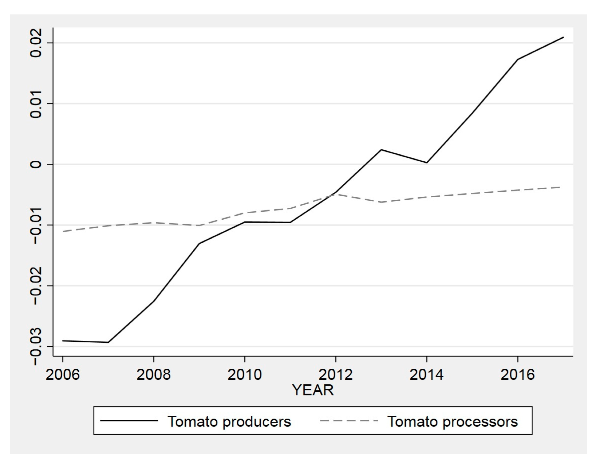
We obtained significant technological change estimate for tomato production. The results indicate that the technological change is negative; however, the technological regression decelerates over time. In particular, Figure 1 shows that the negative technological change turns out to be positive at the end of the analyzed period. This may imply increased investment activities in the second half of the analyzed period. Moreover, we do not reject Hicks’ neutral technological change; in other words, technological change is not factor biased.

Table 3. The distribution of technological change. Source: authors’ calculations.

Level	Min.	First Q	Median	Mean	Third Q	Max.	Std. D.
Tomato producers	−0.090	−0.029	−0.014	−0.014	0.001	0.063	0.022
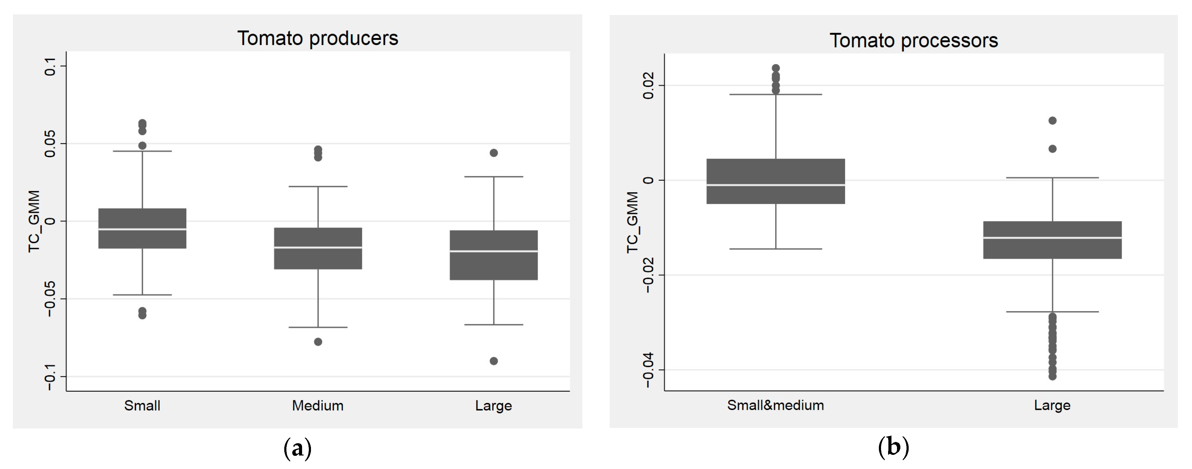
Tomato processors	−0.041	−0.012	−0.006	−0.006	−0.001	0.024	0.010

provides the distribution of the technological change, showing that the technological regression is, to a certain extent, characteristic of three-quarters of the tomato producers. Figure 2 provides the distribution according to size. We can observe that medium and large producers seem to be characterized by higher technological regression, although the differences are not statistically significant. The same holds for tomato processors, as we do not observe any significant differences among the processors’ size groups. In particular, the figures show that the majority of the tomato processors have not experienced any technological changes.

3.2. Distribution of Scale Efficiency and Efficiency of Input Use

Table 4. Scale efficiency. Source: authors’ calculations.

Level	Min.	First Q	Median	Mean	Third Q	Max.	Std. D.	t-Test (H0: RTS=1)
Tomato producers	0.814	1.099	1.281	1.387	1.591	2.611	0.389	25.929 (Pr(|T| > |t|) = 0.0000)
Tomato processors	0.866	0.978	1.011	1.009	1.040	1.170	0.045	5.656 (Pr(|T| > |t|) = 0.0000)

presents the distribution of tomato producers’ and processors’ returns to scale. As already stated, the producers are characterized by considerably high increasing returns to scale, which holds for the whole sample. Moreover, the figures of the third quartile show that this group of farmers is considerably scale inefficient. We thus can observe that the producer sample is characterized by higher heterogeneity in scale efficiency compared to processors. The majority of the processors operate with almost constant returns to scale.

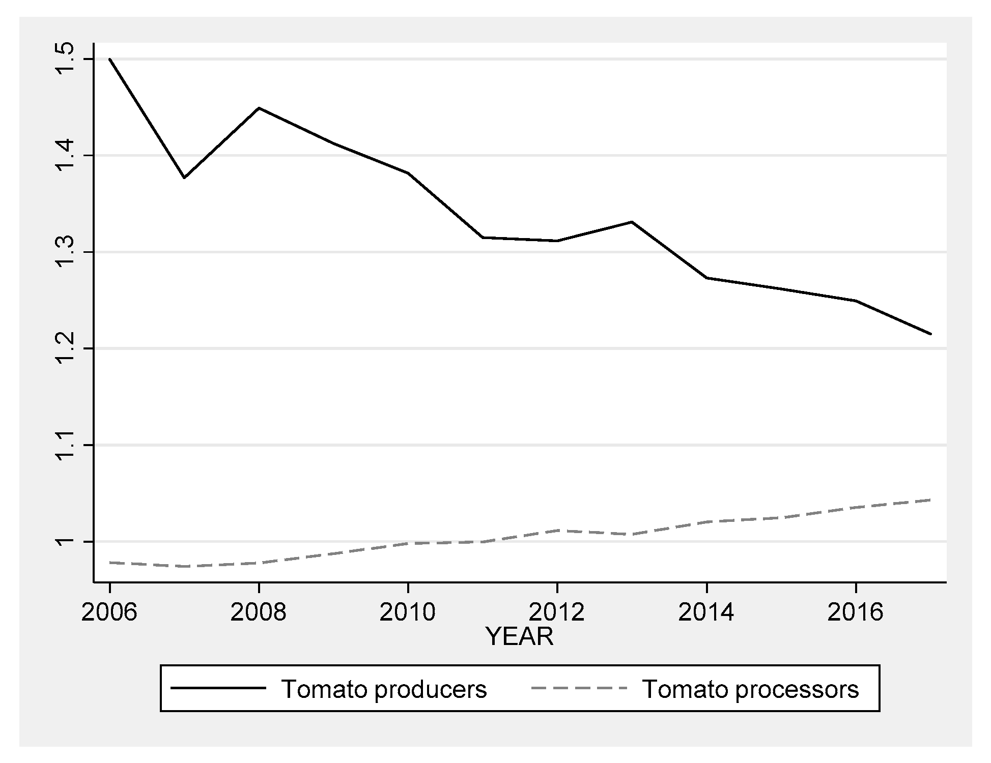
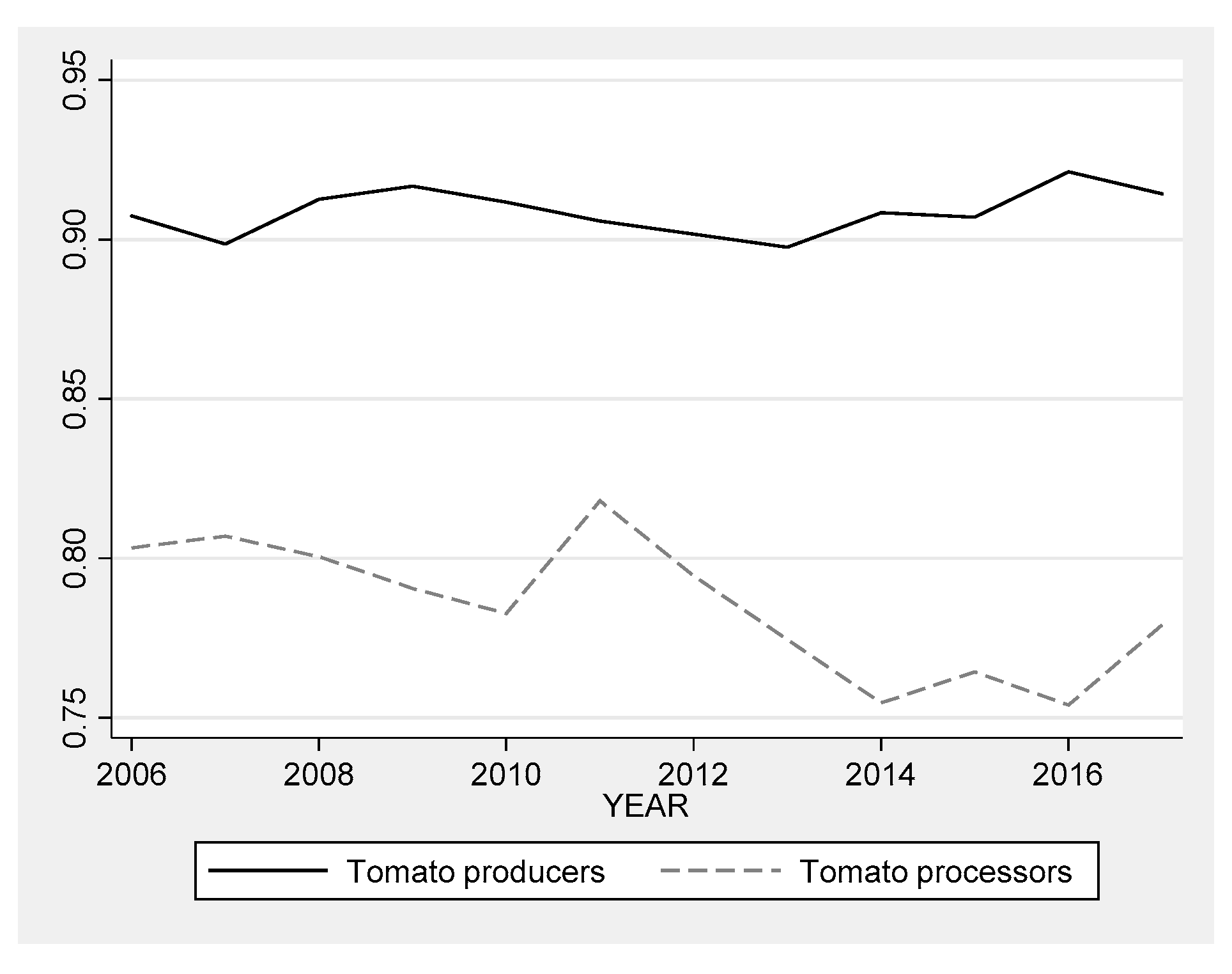
Figure 3 provides the dynamics of the scale efficiency. We can observe considerable improvements to the producers’ scale efficiency; that is, unexploited economies of scale reduced substantially in tomato production over the 2006–2017 period. In the case of tomato processors, we do not observe any significant change, which is an expected outcome when the processors operate with optimal size of production.

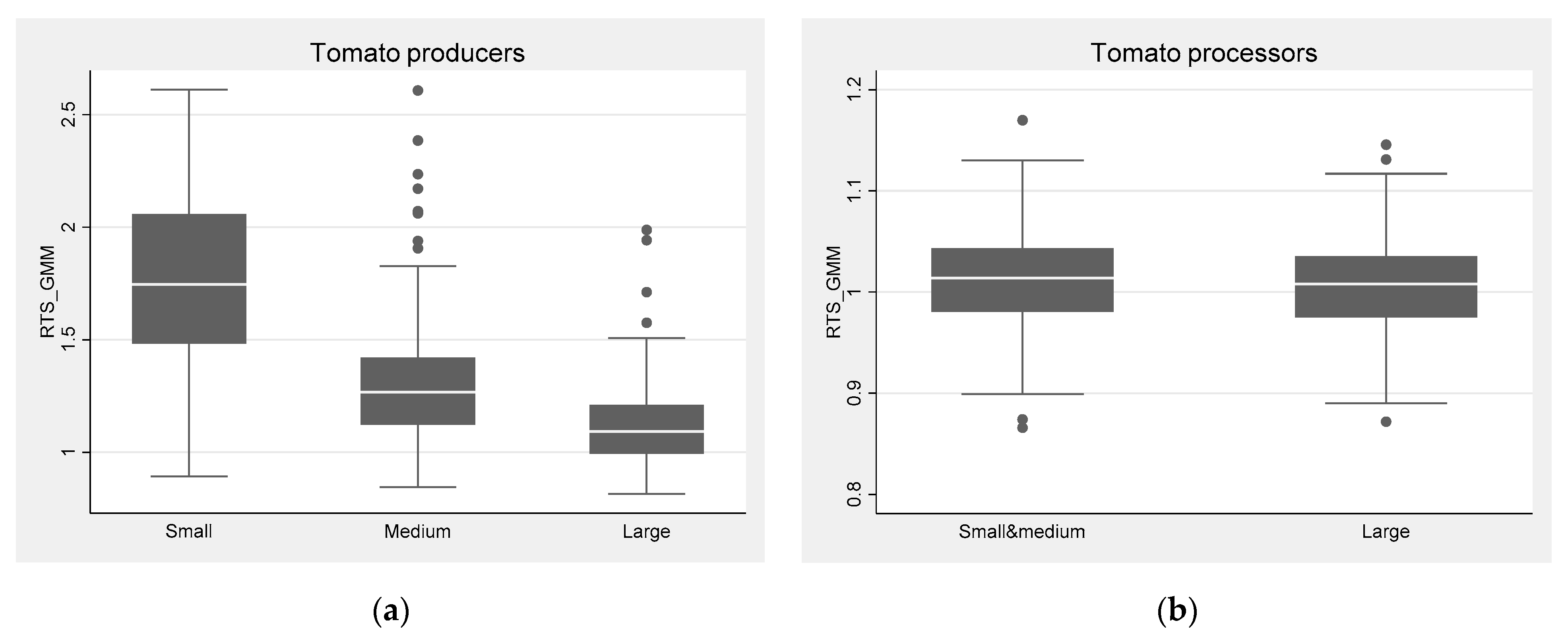
The distribution of economies of scale according to size (Figure 4) provides the expected results for the tomato producers and confirms our findings for the tomato processors. In particular, we observe a positive association between improvements in economies of scale and the size of the tomato producer. Whereas small producers exhibit high increasing returns to scale, large producers are close to a constant return to scale, i.e., an optimal scale of operations. Small, medium as well as large tomato processors operate at the optimal size.

Overall technical efficiency is of a similar level in tomato production and processing and indicates considerable space for improvements. The mean of overall technical efficiency in production is 81.2% and 77.6% in processing (

Table 5. Technical efficiency. Source: authors’ calculations.

Tomato Producers
	Min.	First Q	Median	Mean	Third Q	Max.	Std. D.
Overall	0.644	0.790	0.817	0.812	0.839	0.903	0.040
Transient	0.700	0.896	0.913	0.909	0.926	0.965	0.028
Persistent	0.750	0.876	0.899	0.893	0.915	0.951	0.032
Tomato Processors
	Min.	First Q	Median	Mean	Third Q	Max.	Std. D.
Overall	0.600	0.716	0.782	0.776	0.837	0.962	0.081
Transient	0.605	0.723	0.789	0.785	0.845	0.975	0.081
Persistent	0.954	0.986	0.990	0.988	0.992	0.997	0.006

). That is, the tomato producers and processors operating on the technological frontier have significantly lower costs, by approximately 19% and 22%, as compared to the sample average, respectively. This represents a considerable competitive advantage for efficient producers and processors.

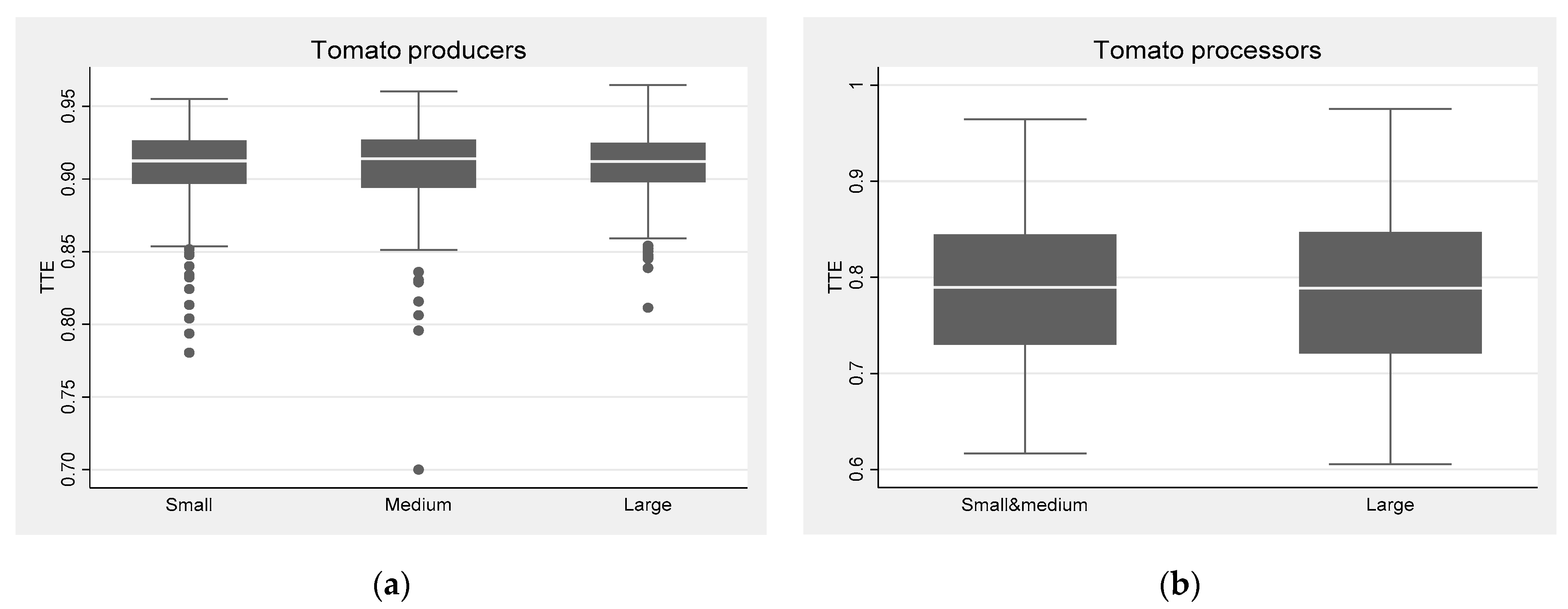
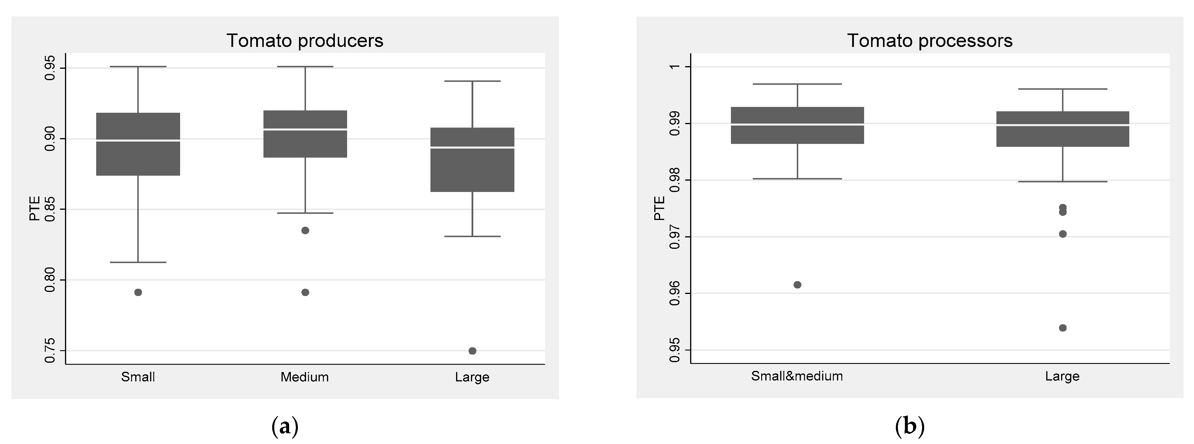
The persistent technical inefficiency estimates indicate that, compared to tomato processors, tomato producers are characterized by considerably high levels of farm management systematic failures due to optimal resource use. On the other hand, transient inefficiency is substantially low in tomato production compared to tomato processing. In particular, the technical inefficiencies in tomato processing are due to transient components, and we do not observe significant systematic failures in optimal resource use in tomato processing. Moreover, Figure 5 does not suggest any significant change in efficiency of input use during the study period.

Finally, we do not observe significant differences among size groups of tomato producers and processors in overall technical efficiency (Figure 6). The same holds for persistent technical efficiency (Figure 7).

3.3. Productivity Dynamics

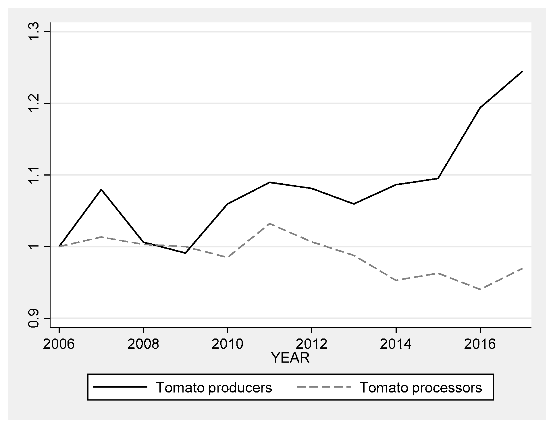
Figure 8 shows that we can observe significant productivity improvements in tomato production, although the opposite is true for tomato processing. Whereas the productivity increased by more than 20% in tomato production as compared to the initial year of 2006, the productivity of tomato processors slightly decreased, by 3%.

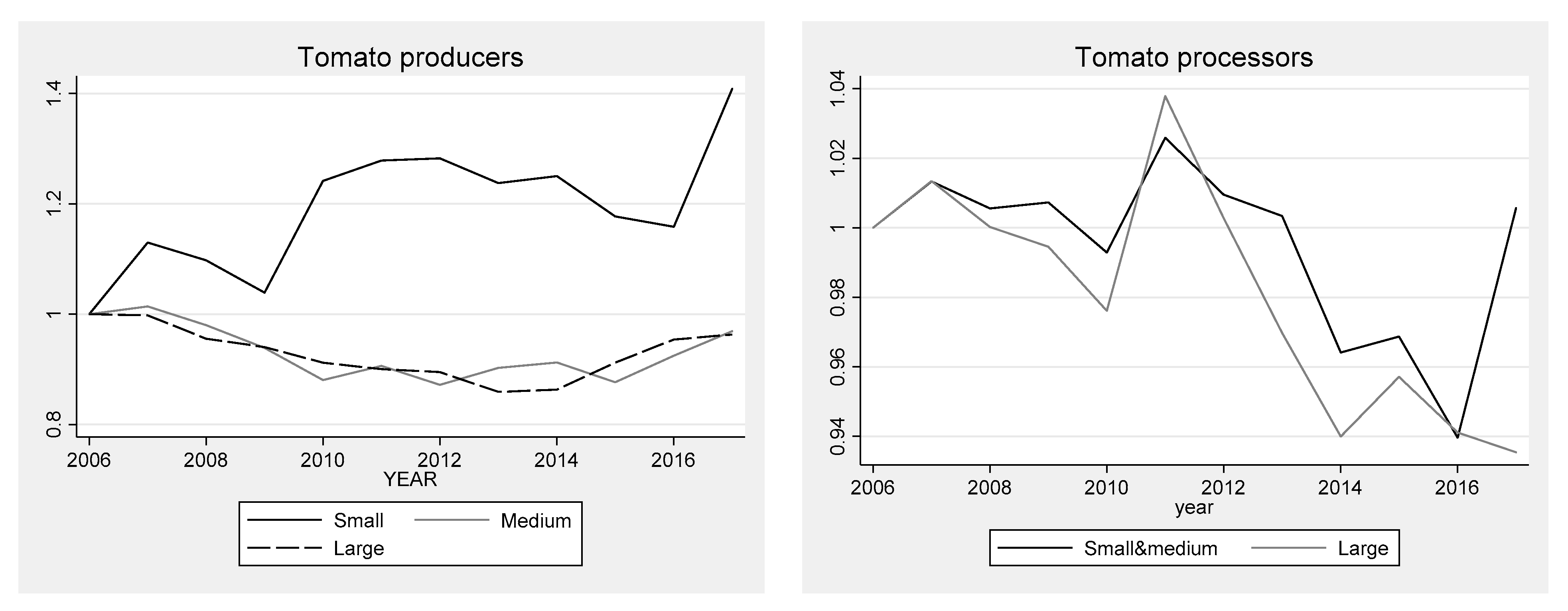
Figure 9 indicates that the productivity growth in tomato production was driven by the group of small producers. With respect to our forgoing analysis, it is not surprising that the breakdown of TFP revealed that the main source of productivity increases in this group was a scale component. That is, the improvements in the scale of operations (scale efficiency) were the driver of TFP growth for the group of small tomato producers. Middle and large producers experienced similar development as the small producers, that is, a slight decrease in productivity.

4. Discussion and Conclusions

This study evaluates productivity dynamics and identifies sources that induce productivity changes in Italian tomato production and processing. The use of the latest advances in stochastic frontier analysis can obtain unbiased estimates of production and processing technology as well as efficiency and productivity measures. As opposed to other studies, this study contributes to the literature by providing a productivity and efficiency comparison of two stages of the tomato value chain. Moreover, the research provides a breakdown of technical efficiency and divides it into transient and persistent components, which differs from most of the other similar research to date.

The current study results provide a comprehensive agro-food chain perspective encompassing actors at the agricultural and processing level. They point out the differences and the similarities that each actor reports over time. This overarching and food system perspective contributes to the definition of evidence-based results. This study may contribute to the definition of technical and policy interventions aimed at targeting the productivity change drivers in the tomato food value chain.

Results show that technological change is not a significant source of productivity growth in tomato processing. On the other hand, however, tomato production is characterized by negative, decelerating technological change that reversed to become positive at the end of the analyzed period. Moreover, we do not observe significant differences among producers across the different size groups.

The estimates suggest that the producers exhibit considerable economies of scale, whereas the tomato processors are characterized by constant returns to scale. That is, whereas tomato processors have optimal production sizes, tomato producers experience considerably high scale inefficiencies, with these inefficiencies being more pronounced in the group of smaller tomato producers. In particular, the smaller producers exhibit high increasing returns to scale compared to the larger producers, which display near constant returns to scale, i.e., an optimal scale of operations. Producer dimensions have an impact on the efficiency level. Results suggest there may be greater room for efficiency improvements among smaller compared to larger producers. However, larger farmers may still benefit from investments in education and training, advice and information as well as increased sensitivity and knowledge regarding environmental and social sustainability. These may complete the set of sustainability dimensions agriculture will increasingly have to ensure. The use of different technologies and improved efficiency means aiming for increasing production, productivity and profits in a sustainable way. This is particularly relevant to tomato production as it is a high water consuming agricultural sector. Technological developments are rapidly evolving and require new managerial practices, able to manage multidisciplinary technologies. Results show that producers would benefit from technological advancements, yet there may be some reluctance as information on the costs and benefits of adopting technologies in agriculture is often imperfect. This would lead to optimization of resource utilization by tomato farmers.

Overall, the technical efficiency estimates indicate considerable room for improvements to be made. The mean of the overall technical efficiency for production is 81.2% and 77.6% for processing, which provides significant room for cost reductions if the producers and processors were to operate with frontier technologies. Moreover, persistent technical inefficiency is more pronounced in tomato production as compared to tomato processing, suggesting the presence of high levels of systematic farm management failures. These results reflect the continuous investments in innovation and technology that processors have carried out over time. Innovative technologies have been tested over time and in various geographical contexts providing benefits for processors at the global level. Then again, the global competition has pushed the need to increase commercial competitiveness. Thus, the Italian processing industry has increased production efficiency and widened the adoption of the processing technologies available. Nevertheless, these research results support that there is room for improvement.

Finally, the current study observed significant productivity improvements for tomato production. This is, however, not the case for tomato processing, which experienced minor productivity changes over the analyzed period. Moreover, the results reveal that the productivity growth in tomato production was driven by a group of small producers and, in particular, by considerable improvements in scale efficiency.

References

- Ronga, D.; Francia, E.; Rizza, F.; Badeck, F.-W.; Caradoniaa, F.; Montevecchi, G.; Pecchioni, N. Changes in yield components, morphological, physiological and fruit quality traits in processing tomato cultivated in Italy since the 1930’s. Sci. Hortic. 2019, 257, 108726. [Google Scholar] [CrossRef]
- Pahlavan, R.; Omid, M.; Akram, A. Energy use efficiency in greenhouse tomato production in Iran. Energy 2011, 36, 6714–6719. [Google Scholar] [CrossRef]
- Cammaranoa, D.; Ronga, D.; Di Mola, I.; Mori, M.; Parisi, M. Impact of climate change on water and nitrogen use efficiencies of processing tomato cultivated in Italy. Agric. Water Manag. 2020, 241, 106336. [Google Scholar] [CrossRef]
- Francaviglia, R.; Di Bene, C. Deficit Drip Irrigation in Processing Tomato Production in the Mediterranean Basin. A Data Analysis for Italy. Agriculture 2019, 9, 79. [Google Scholar] [CrossRef] [Green Version]
- Giuliani, M.M.; Gatta, G.; Cappelli, G.; Gagliardi, A.; Donatelli, M.; Fanchini, D.; De Nart, D.; Mongiano, G.; Bregaglio, S. Identifying the most promising agronomic adaptation strategies for the tomato growing systems in Southern Italy via simulation modelling. Eur. J. Agron. 2019, 111, 125937. [Google Scholar] [CrossRef]
- Boccia, F.; Di Donato, P.; Covino, D.; Poli, A. Food waste and bio-economy: A scenario for the Italian tomato market. J. Clean. Prod. 2019, 227, 424–433. [Google Scholar] [CrossRef]
- FAOSTAT. Crops. Available online: http://www.fao.org/faostat/en/#data/QC (accessed on 23 July 2021).
- EUROSTAT. Crop Production in National Humidity. Available online: http://www.fao.org/faostat/en/#data/QC (accessed on 23 July 2021).
- Capobianco-Uriarte, M.D.L.M.; Aparicio, J.; De Pablo-Valenciano, J.; Casado-Belmonte, M.D.P. The European tomato market. An approach by export competitiveness maps. PLoS ONE 2021, 16, e0250867. [Google Scholar] [CrossRef] [PubMed]
- The World Processing Tomato Council. The 2020 Processed Tomato Yearbook. Available online: http://www.tomatonews.com/pdf/yearbook/2020/index.html#1 (accessed on 23 July 2021).
- Fragni, R.; Trifirò, A.; Nucci, A.; Seno, A.; Allodi, A.; Di Rocco, M. Italian tomato-based products authentication by multi-element approach: A mineral elements database to distinguish the domestic provenance. Food Control 2018, 93, 211–218. [Google Scholar] [CrossRef]
- De Marco, I.; Riemma, S.; Iannone, R. Uncertainty of input parameters and sensitivity analysis in life cycle assessment: An Italian processed tomato product. J. Clean. Prod. 2018, 177, 315–325. [Google Scholar] [CrossRef]
- Lombardia, A.; Verneaua, F.; Lombardi, P. Development and Trade Competitiveness of the Italian Tomato Sector. Agric. Econ. Rev. 2016, 17, 5–19. [Google Scholar] [CrossRef]
- Latruffe, L. Competitiveness, Productivity and Efficiency in the Agricultural and Agri-Food Sectors; OECD Food, Agriculture and Fisheries Papers, No.: 30; OECD Publishing: Paris, France, 2010. [Google Scholar] [CrossRef]
- O’Donnell, C.J. Nonparametric estimates of the components of productivity and profitability change in U.S. agriculture. Am. J. Agric. Econ. 2012, 94, 873–890. [Google Scholar] [CrossRef]
- Blandinières, F.; Dürr, N.; Frübing, S.; Heim, S.; Pieters, B.; Janger, J.; Peneder, M. Measuring Competitiveness. Available online: https://ec.europa.eu/docsroom/documents/28181/attachments/1/translations/en/renditions/pdf (accessed on 24 July 2021).
- Murray, A. Partial versus Total Factor Productivity Measures: An Assessment of their Strengths and Weaknesses. Int. Product. Monit. 2016, 31, 113–126. [Google Scholar]
- Wimmer, S.G.; Sauer, J. Diversification versus specialization: Empirical evidence on the optimal structure of European dairy farms. In Proceedings of the 56th Annual Conference of the GEWISOLA “Agricultural and Food Economy: Regionally Connected and Globally Successful”, Bonn, Germany, 28–30 September 2016. [Google Scholar]
- Kumbhakar, S.C.; Wang, H.-J.; Horncastle, A.P. A Practitioner’s Guide to Stochastic Frontier Analysis Using Stata; Cambridge University Press: New York, NY, USA, 2015; 359p. [Google Scholar]
- De Roest, K.; Ferrari, P.; Knickel, K. Specialisation and economies of scale or diversification and economies of scope? Assessing different agricultural development pathways. J. Rural. Stud. 2017, 59, 222–231. [Google Scholar] [CrossRef]
- Koopmans, T.C. Analysis of Production as an Efficient Combination of Activities. In Activity Analysis of Production and Allocation; Koopmans, T.C., Ed.; John Wiley & Sons, Inc.: London, UK, 1951; pp. 33–57. [Google Scholar]
- Farrell, M.J. The Measurement of Productive Efficiency. J. R. Stat. Soc. 1957, 120, 253–290. [Google Scholar] [CrossRef]
- Dimara, E.; Skuras, D.; Tsekouras, K.; Tzelepis, D. Productive efficiency and firm exit in the food sector. Food Policy 2008, 33, 185–196. [Google Scholar] [CrossRef]
- Njuki, E.; Bravo-Ureta, B.E. The Economic Costs of Environmental Regulation in U.S. Dairy Farming: A Directional Distance Function Approach. Am. J. Agric. Econ. 2015, 97, 1087–1106. [Google Scholar] [CrossRef] [Green Version]
- Filippini, M.; Greene, W.H. Persistent and Transient Productive Inefficiency: A Maximum Simulated Likelihood Approach. J. Product. Anal. 2016, 45, 187–196. [Google Scholar] [CrossRef]
- Benedetti, I.; Branca, G.; Zucaro, R. Evaluating input use efficiency in agriculture through a stochastic frontier production: An application on a case study in Apulia (Italy). J. Clean. Prod. 2019, 236, 117609. [Google Scholar] [CrossRef]
- Khan, H.; Ali, F. Measurement of productive efficiency of tomato growers in Peshawar, Pakistan. Agric. Econ. 2013, 59, 381–388. [Google Scholar] [CrossRef]
- Ogunniyi, L.T.; Oladejo, J.A. Technical Efficiency of tomato production in Oyo State Nigeria. Agric. Sci. Res. J. 2011, 1, 84–91. [Google Scholar]
- Tabe-Ojong, M.P.; Molua, E.L. Technical Efficiency of Smallholder Tomato Production in Semi-Urban Farms in Cameroon: A Stochastic Frontier Production Approach. J. Manag. Sustain. 2017, 7, 27–35. [Google Scholar] [CrossRef] [Green Version]
- Najjuma, E.; Kavoi, M.M.; Mbeche, R. Assessment of technical efficiency of open field tomato production in Kiambu country, Kenya (Stochastic frontier approach). J. Agric. Sci. Technol. 2016, 17, 21–39. [Google Scholar]
- Zalkuw, J.; Singh, R.; Pardhi, R.; Gangwar, A. Analysis of Technical Efficiency of Tomato Production in Adamawa State, Nigeria. Int. J. Agric. Environ. Biotechnol. 2014, 7, 645–650. [Google Scholar] [CrossRef]
- Khan, R.E.A.; Ghafar, S. Technical Efficiency of Tomato Production: A Case Study of District Peshawar (Pakistan). World Appl. Sci. J. 2013, 28, 1389–1392. [Google Scholar] [CrossRef]
- Adenuga, A.H.; Muhammad-Lawal, A.; Rotimi, O.A. Economics and Technical Efficiency of Dry Season Tomato Production in Selected Areas in Kwara State, Nigeria. Agris Online Pap. Econ. Inform. 2013, 5, 11–19. [Google Scholar] [CrossRef]
- Frangu, B.; Popp, J.S.; Thomsen, M.; Musli, A. Evaluating Greenhouse Tomato and Pepper Input Efficiency Use in Kosovo. Sustainability 2018, 10, 2768. [Google Scholar] [CrossRef] [Green Version]
- Yang, Q.; Zhu, Y.; Wang, J. Adoption of drip fertigation system and technical efficiency of cherry tomato farmers in Southern China. J. Clean. Prod. 2020, 275, 123980. [Google Scholar] [CrossRef]
- Rinaldi, M.; Garofalo, P.; Vonella, V.A. Productivity and Water Use Efficiency in Processing Tomato under Deficit Irrigation in Southern Italy. Acta Horticulturae 2014, 1081, 97–104. [Google Scholar] [CrossRef]
- Gebremariam, H.G.; Weldegiorgis, L.G.; Tekle, A.H. Efficiency of male and female as irrigated onion growers. International J. Veg. Sci. 2018, 25, 571–580. [Google Scholar] [CrossRef]
- Gwebu, J.Z.; Matthews, N. Metafrontier analysis of commercial and smallholder tomato production: A South African case. South Afr. J. Sci. 2018, 114, 2017–2058. [Google Scholar] [CrossRef]
- Murthy, D.S.; Sudha, M.; Hegde, M.R.; Dakshinamoorthy, V. Technical efficiency and its determinants in tomato production in Karnataka, India: Data envelopment analysis (DEA) approach. Agric. Econ. Res. Rev. 2009, 22, 215–224. [Google Scholar] [CrossRef]
- Ghodsi, M.; Mohammadi, H. Study of Tomato Processing Efficiency in Fars Province. Agric. Econ. Res. 2009, 1, 1–24. [Google Scholar]
- Kumbhakar, S.C.; Tsionas, E.G. Firm heterogeneity, persistent and transient technical inefficiency: A generalized true random effects model. J. Appl. Econom. 2012, 29, 110–132. [Google Scholar] [CrossRef]
- Čechura, L.; Žáková Kroupová, Z. Technical Efficiency in the European Dairy Industry: Can We Observe Systematic Failures in the Efficiency of Input Use? Sustainability 2021, 13, 1830. [Google Scholar] [CrossRef]
- O’Donnell, C.J. Measuring and decomposing agricultural productivity and profitability change. Aust. J. Agric. Resour. Econ. 2010, 54, 527–560. [Google Scholar] [CrossRef] [Green Version]
- Coelli, T.J.; Rao, D.S.P.; O’Donnell, C.J.; Battese, G.E. An Introduction to Efficiency and Productivity Analysis, 2nd ed.; Springer: New York, NY, USA, 2005. [Google Scholar]
- Bokusheva, B.; Čechura, L. Evaluating Dynamics, Sources and Drivers of Productivity Growth at the Farm Level; OECD Food, Agriculture and Fisheries Papers, No. 106; OECD Publishing: Paris, France, 2017. [Google Scholar]
- Caves, D.W.; Christensen, L.R.; Diewert, W.E. Multilateral comparisons of output, input and productivity using superlative index numbers. Econ. J. 1982, 92, 73–86. [Google Scholar] [CrossRef]
- Fried, H.O.; Knox Lovell, C.A.; Schmidt, S.S. The Measurement of Productive Efficiency and Productivity Growth, 1st ed.; Oxford University Press: New York, NY, USA, 2008. [Google Scholar]
- Shephard, R.W. Cost and Production Functions, 1st ed.; Princeton University Press: Princeton, NJ, USA, 1953. [Google Scholar]
- Chambers, R.G.; Chung, Y.; Färe, R. Profit, Directional Distance Functions, and Nerlovian Efficiency. J. Optim. Theory Appl. 1998, 98, 351–364. [Google Scholar] [CrossRef]
- Diewert, W. Exact and Superlative Index Numbers. J. Econom. 1976, 4, 115–145. [Google Scholar] [CrossRef]
- Čechura, L.; Grau, A.; Hockmann, H.; Levkovych, I.; Kroupová, Z. Catching up or falling behind in Eastern European agriculture—The case of milk production. J. Agric. Econ. 2017, 6, 206–227. [Google Scholar] [CrossRef]
- Sipiläinen, T. Sources of productivity growth on Finnish dairy farms—Application of input distance function. Acta Agric. Scand. Sect. C. 2007, 4, 65–67. [Google Scholar] [CrossRef]
- Kumbhakar, S.C.; Lien, G.; Hardaker, J.B. Technical efficiency in competing panel data models: A study of Norwegian grain farming. J. Product. Anal. 2014, 41, 321–337. [Google Scholar] [CrossRef]
- Arellano, M.; Bover, O. Another look at the instrumental variable estimation of error-components models. J. Econom. 1995, 68, 29–51. [Google Scholar] [CrossRef] [Green Version]
- Blundell, R.; Bond, S. Initial conditions and moment restrictions in dynamic panel data models. J. Econom. 1998, 87, 115–143. [Google Scholar] [CrossRef] [Green Version]
- Arellano, M.; Bond, S. Some Tests of Specification for Panel Data: Monte Carlo Evidence and an Application to Employment Equations. Rev. Econ. Stud. 1991, 58, 277. [Google Scholar] [CrossRef] [Green Version]
Figure 1.
Development of technological change. Source: authors’ calculations.
Figure 2.
Distribution of technological change; (a) tomato producers and (b) tomato processors. Source: authors’ calculations.
Figure 3.
Development of returns to scale. Source: authors’ calculations.
Figure 4.
Distribution of returns to scale; (a) tomato producers and (b) tomato processors. Source: authors’ calculations.
Figure 5.
Development of technical efficiency. Source: authors’ calculations.
Figure 6.
Distribution of transient technical efficiency; (a) tomato producers and (b) tomato processors. Source: authors’ calculations.
Figure 7.
Distribution of persistent technical efficiency; (a) tomato producers and (b) tomato processors. Source: authors’ calculations.
Figure 8.
TFP growth in tomato production and processing (2006=100). Source: authors’ calculations.
Figure 9.
TFP dynamics according to the size (2006=100). Source: authors’ calculations.