An Automatic Light Stress Grading Architecture Based on Feature Optimization and Convolutional Neural Network

Abstract

The identification of light stress is crucial for light control in plant factories. Image-based lighting classification of leafy vegetables has exhibited remarkable performance with high convenience and economy. Convolutional Neural Network (CNN) has been widely used for crop image analysis because of its architecture, high accuracy and efficiency. Among them, large intra-class differences and small inter-class differences are important factors affecting crop identification and a critical challenge for fine-grained classification tasks based on CNN. To address this problem, we took the Lettuce (Lactuca sativa L.) widely grown in plant factories as the research object and constructed a leaf image set containing four stress levels. Then a light stress grading model combined with classic pre-trained CNN and Triplet loss function is constructed, which is named Tr-CNN. The model uses the Triplet loss function to constrain the distance of images in the feature space, which can reduce the Euclidean distance of the samples from the same class and increase the heterogeneous Euclidean distance. Multiple sets of experimental results indicate that the model proposed in this paper (Tr-CNN) has obvious advantages in light stress grading dataset and generalized dataset.

1. Introduction

The identification and control of the light environment is the key to high-yield and high-quality production of crops in plant factories, and a crucial requirement for energy conservation. Early recognition of crop light stress presents a critical part for light environment control in plant factories, but also an important requirement for early detection and prevention of crop damage.

Crops are very sensitive to light intensity. Strong or weak light will induce changes to plant growth structure, particularly leaf surface [1,2]. Leafy vegetables are widely planted in plant factories. While light intensity has a major impact on both the yield and quality of leafy vegetables. The experiment from Hao et al. [3] evidenced that different light intensities contributed to huge differences in fresh shoot weight, fresh root weight, anthocyanin, and soluble sugar of purple Bok Choy. The research of Kleinhenz et al. [4] also showed that lettuce is very sensitive to light intensity. Different light intensities not only have a greater impact on the anthocyanins and chlorophylls of lettuce, but also bring obvious visual separability. This visual separability can be expressed through images. Therefore, it would be feasible to grade light stress through images.

There are already many image formats available for stress analysis. Spectral image is one of the commonly used data formats for this area. Reum et al. [5] established a set of image processing methods to assess maize plant nitrogen stress based on multi-spectral images to find information related to nitrogen levels. Nowadays, RGB images have been applied in more works with the development of high-throughput phenotyping (HTP). RGB images have the advantages of convenience, high-speed and low-cost relative to spectral images. It provides the physical properties of plants, such as canopy vitality, leaf color, leaf texture, size and shape information. Chen et al. [6] analyzed the response of wheat to drought stress based on RGB images. Esgario et al. [7] designed a practical system to recognize the severity of stress caused by biological agents in coffee leaves based on RGB images. In contrast, the acquisition of RGB images is more convenient. Users can obtain images through monitoring equipment, cameras, or mobile phones. This low-cost and convenient image acquisition method is more conducive to the universal application of models.

Many primary studies have been done and published on stress analysis based on images. Early works were mostly based on traditional image processing methods [8,9,10] which have greatly advanced the development of image crop stress analysis. However, these methods rely on handcrafted features, which not only limits the expression of hidden features, but also is susceptible to individual visual differences. Therefore, they have certain limitations in terms of accuracy improvement. The vigorous development of artificial intelligence has led to the development of image analysis. Inspired by the great success of deep learning in various computer vision tasks, the application of deep convolutional neural network (DCNN) models to crop stress phenotypes has become increasingly popular [11,12,13].

Image-based stress classification is usually based on leaves, which belongs to the category of fine-grained visual classification (FGVC) [14]. FGVC is also called Sub-Category Recognition. Its purpose is to divide the coarse-grained categories into more detailed sub-categories. The investigation of crop fine-grained image classification has been one of the priority fields in crop stress analysis, pest analysis, fruit maturity recognition in recent years. Only small local differences usually are used to distinguish different classes as the differences between categories of fine-grained images are subtler. In our task of light intensity stress classification, a certain threshold is usually chosen to define two adjacent classes. This will lead to insignificant differences between classes and insufficient “aggregation” of features within one class, which is also a huge problem faced by FGVC. Many scholars have done a lot of researches on it. Improving the learning of local details is a common way to solve FGVC problems. For instance, learning the local discriminative features using attention mechanism [15,16] or amplifying the details of the input images by multi-scale input network [17]. Despite these methods have achieved good results in extracting fine-grained features, they have not fundamentally solved the problem of differences between and within categories.

One effective way to deal with small inter-class variance and large intra-class variance is metric learning. It uses the similarity function to project images with similar content onto adjacent positions on a manifold, which in turn maps images with different semantic backgrounds separately. This feature mapping method enables the “separation” of inter-class features and the “aggregation” of intra-class features. With the vigorous development of deep neural networks (DNN), metric learning has shifted from learning distance functions to deep feature embeddings that are more suitable for simple distance functions, such as Euclidean distance or cosine distance metric learning. Deep metric learning is vastly used in various target detection e.g., as face recognition, target tracking. Many widely applicable loss functions have been developed for deep metric learning, such as contrast loss, triplet loss, quadruplet loss, etc. Their common goal is to encourage samples from the same category to be closer and separate samples from different categories in a projected feature space.

Inspired by the above research, in this work, we present a novel light stress grading method (we named Tr-CNN) combined with deep metric learning and CNN. It learns embedding features at a fine-grained level through triplet loss function. By minimizing the loss of triples, the distance between different classes in the feature space is always greater than the distance between the same class by a certain threshold. The CNN model pre-trained on ImageNet was chosen as a baseline to solve the problem of slow convergence and overfitting in the triple mining process.

In general, the contributions of this work are as follows:

• The classification architecture based on Triplet loss function and pre-trained CNN model was innovatively proposed and implemented on the new task of light stress grading.
• The model was implemented on our own public dataset. The image set can be download from https://drive.google.com/drive/folders/1Mz2YQ-Sm7RL-qa4tHvJ89_4rnoHq-gkw (accessed on 31 December 2020) or https://pan.baidu.com/s/19hMRMIAHY9_0rHDeS_HxvQ (Extraction code: tcnn) (accessed on 31 December 2020).
• We determined the parameters through multiple sets of experiments, and evaluated the applicability of the model through experiments on the generalized dataset. Experimental results show that Tr-CNN has obvious advantages in more fine-grained image classification.

2. Related Works

Light stress grading based on leaf images belongs to the category of FGVC. Therefore, in this section, we first reviewed and summarized the research of FGVC based on CNN. In addition, we made a statement on the core area involved in this paper-metric learning.

2.1. Fine-Grained Visual Classification Based on CNN

FGVC based on CNN is an effective method for processing light intensity stress recognition tasks. The task is to identify the sub-categories under the parent category. The main problem faced by FGVC is:

• The distinguishable features are not obvious, that is, small inter-class differences and large intra-class differences. Especially, when performing classification tasks of the same species, the categories are usually artificially divided according to a threshold, which may lead to insignificant differences between the categories.
• Easy to be affected by factors such as viewing angle, background, occlusion, etc.

Many classic CNN models are applied for FGVC, which has achieved acceptable results in a period [18,19]. But these methods are still limited in solving the above problems. Some improvements are further developed to boost the performance of CNN in fine-grained recognition tasks. We summarize the relevant research into the following parts.

2.1.1. Extracting Distinguishing Local Details

The differences between categories are usually manifested in the local content of the image. For example, crop diseases are generally communicated as illness spots and textures. Therefore, some models improve the separability by extracting discriminative local image patches. Attention mechanism is a viable strategy to highlight local details, which can enhance the expression of interesting features. Wang et al. [20] established a context-aware attention network to detect and classify field pests. Karthik et al. [21] applied attention mechanism on top of the residual deep network, which achieved an overall accuracy of 98% on the validation sets. The powerful recognition and positioning of distinguishable features by the attention mechanism can effectively resist the interference of complex backgrounds, which in turn can promote the accuracy of FGVC.

In addition to the attention mechanism, coding methods based on higher-order features can also locate regions of interest, such as vector of locally aggregated descriptors (VLAD). It aggregates local salient features into a single vector to express the image concisely. Lu et al. [22] proposed a feature encoding mechanism based on CNN and Fisher vector (FV). It tends to highlight subtle objects via filter-specific convolutional representations to provide stronger discrimination for cultivar recognition. Besides, FV is widely used to extract lesion areas in medical images [23,24].

2.1.2. The Method Based on Network Integration

In order to enhance the ability to distinguish subtle features, the input image of a single scale is usually enlarged to different scales, and then sent to a multi-branch network to learn multi-scale features. In our previous work [17], a two-branch network was designed to extract features from intact leaves and leaf patches at the same time, which significantly improved the accuracy of the growth period classification task. Furthermore, a multi-branch network [25] was proposed to extract complete leaves and leaf patches at four scales. Partially enlarged leaf patches provide richer texture and context information, and show better results in the light intensity classification task of lettuce. Wang et al. [20] established a tree structure based on CNN that could progressively learn fine-grained features to distinguish a subset of categories, which can learn more discriminative features.

The above methods learn fine-grained features by positioning, coding, or local zooming of the region of interest, which enormously improves the classification performance of fine-grained images. However, unlike the phenotype induced by biological stresses such as diseases and insect pests, many leaf changes caused by abiotic stresses are usually shown as global features. Therefore, many methods such as attention mechanisms are difficult to locate local regions of interest. In addition, the above methods are all from the input or network level to improve the learning ability of fine-grained features, and do not essentially solve the problem of inter-class and intra-class differences.

2.2. Deep Metric Learning (DML)

As an emerging technique, DML combines deep learning and metric learning. The purpose of metric learning is to reduce or limit the distance between samples of intra-classes, and increase the distance between samples of inter-classes. DML uses the recognition ability of a deep neural network to map the image into a high-dimensional feature space, in which the Euclidean distance (or cosine distance) is used as the measurement between two points. Deep metric learning has achieved many successful applications in the field of computer vision: face recognition [26], face verification [27], image retrieval [28], signature verification [29], pedestrian re-identification [30], etc.

Loss function is a crucial component of DML, that plays a guide in the optimization of the entire network. Deep metric learning was first widely used in face recognition, during which a series of excellent loss functions emerged. Hadsell et al. [31] proposed Contrastive loss, which can effectively deal with the relationship between paired data in the network and increase the inter-class difference in classifiers. Triplet loss was first proposed by Schroff et al. [32] in the FaceNet. It learns the separability between features by calculating the loss of three input images: make the feature distance between the same identity as small as possible, and the distance between different identities as large as possible. Similarly, Wen et al. [33] proposed center loss to constrain the intra-class distance. Compared with triplet loss, it does not restrict the inter-class distance. Chen et al. [34] proposed quadruplet loss, which adds two negative samples to learn representations better, but it also brings greater computing power.

Aside from face recognition and face re-recognition, triplet loss has begun to be applied to other image recognition and image retrieval tasks. Zhang et al. [35] proposed a triplet loss network based on paired images for vehicle re-identification tasks, that achieved better performance than the current level. From Zhang et al. [36], an improved triplet loss function was used to detect changes in aerial remote sensing images. Tang et al. [37] combined triplet loss with a self-designed CNN network-TrafficNet for multi-level traffic state detection.

Triplet loss can express fine-grained features by constraining the similarity between samples, which can be better adapted to fine-grained image classification tasks. In addition, previous research [38,39] shows that triplet loss can adequately manage the imbalance between classes and small samples. However, triplet loss function has not been introduced into the field of crop fine-grained image classification to our knowledge.

In the grading task, different levels are usually divided according to thresholds, which results in unobvious boundaries between adjacent levels. In our task, the response of leaves to light intensity stress is usually expressed on the intact leaf. For the same lettuce variety and same growth environment except for the light intensity, it is difficult for the model to obtain distinguishable characteristics. Therefore, improving the separability between samples through metric learning is an effective solution for grading light intensity stress.

Inspired by the above analysis, triplet loss was used as a loss function to learn embeddings of images with different light intensity levels. The CNN models (ResNet, NasNet, VGGNet, InceptionV3) pre-trained on ImageNet were chosen as the baseline for feature embedding to solve the slow convergence and over-fitting problems.

3. Materials and Methods

3.1. Data Processing

3.1.1. Data Collection

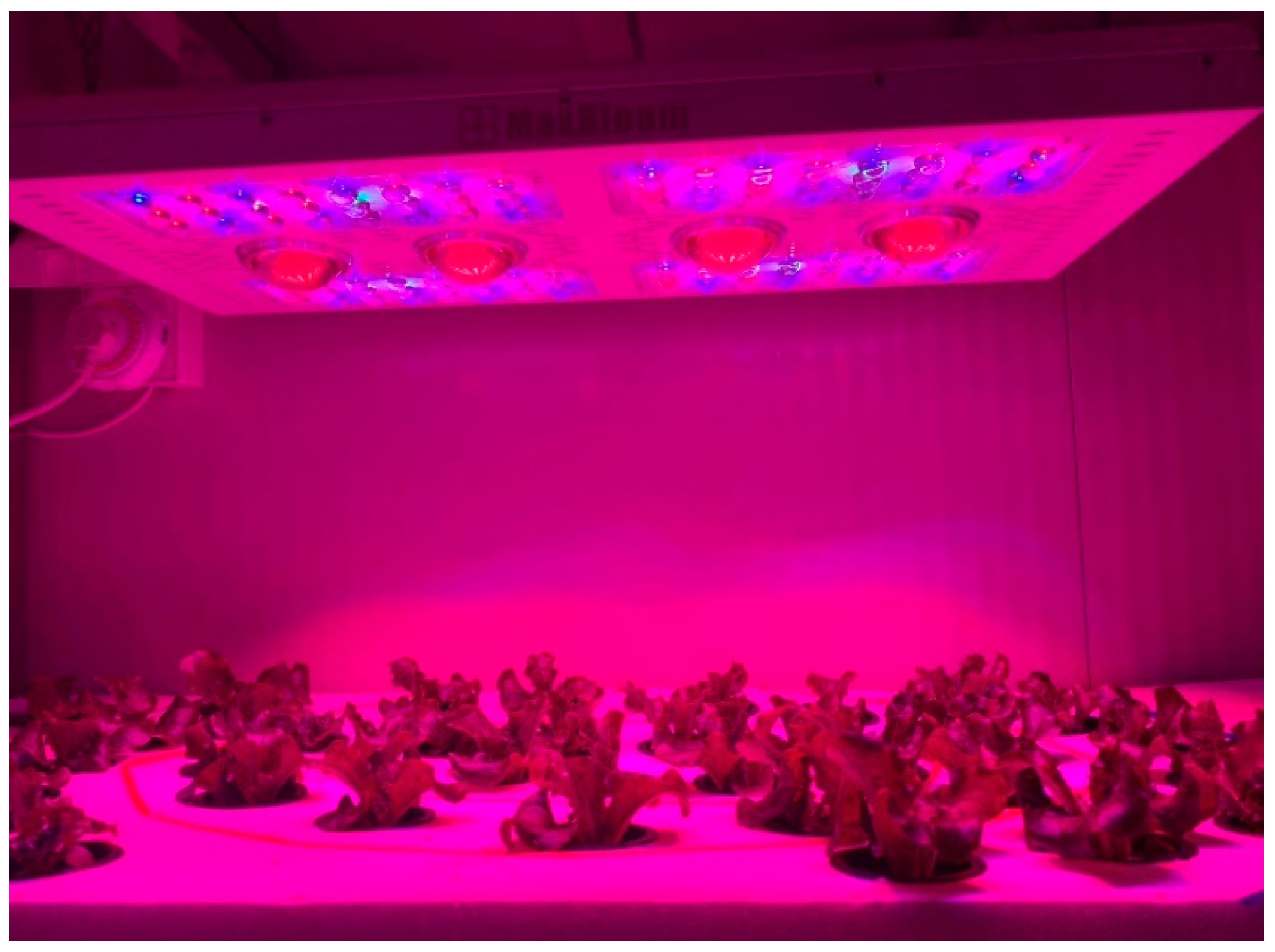
Purple leaf lettuce (Lactuca sativa L., var. zishan) was used as plant materials in our work, which is grown by hydroponics. Indoor experiments were carried out in the plant factory of the College of Information and Electrical Engineering, China Agricultural University, Beijing. Suspended fill light with adjustable light intensity above the hydroponic box was used as the light source (shown in Figure 1). According to the results of previous plant research and the judgment of botanists with relevant work experience [25], lettuce is divided into four stress levels: severe low-light stress (light intensity in 0–100 μmol m⁻² s⁻¹); semi light-limited (100–200 μmol m⁻² s⁻¹); suitable light environment (200–350 μmol m⁻² s⁻¹); high-light stress (350– μmol m⁻² s⁻¹).

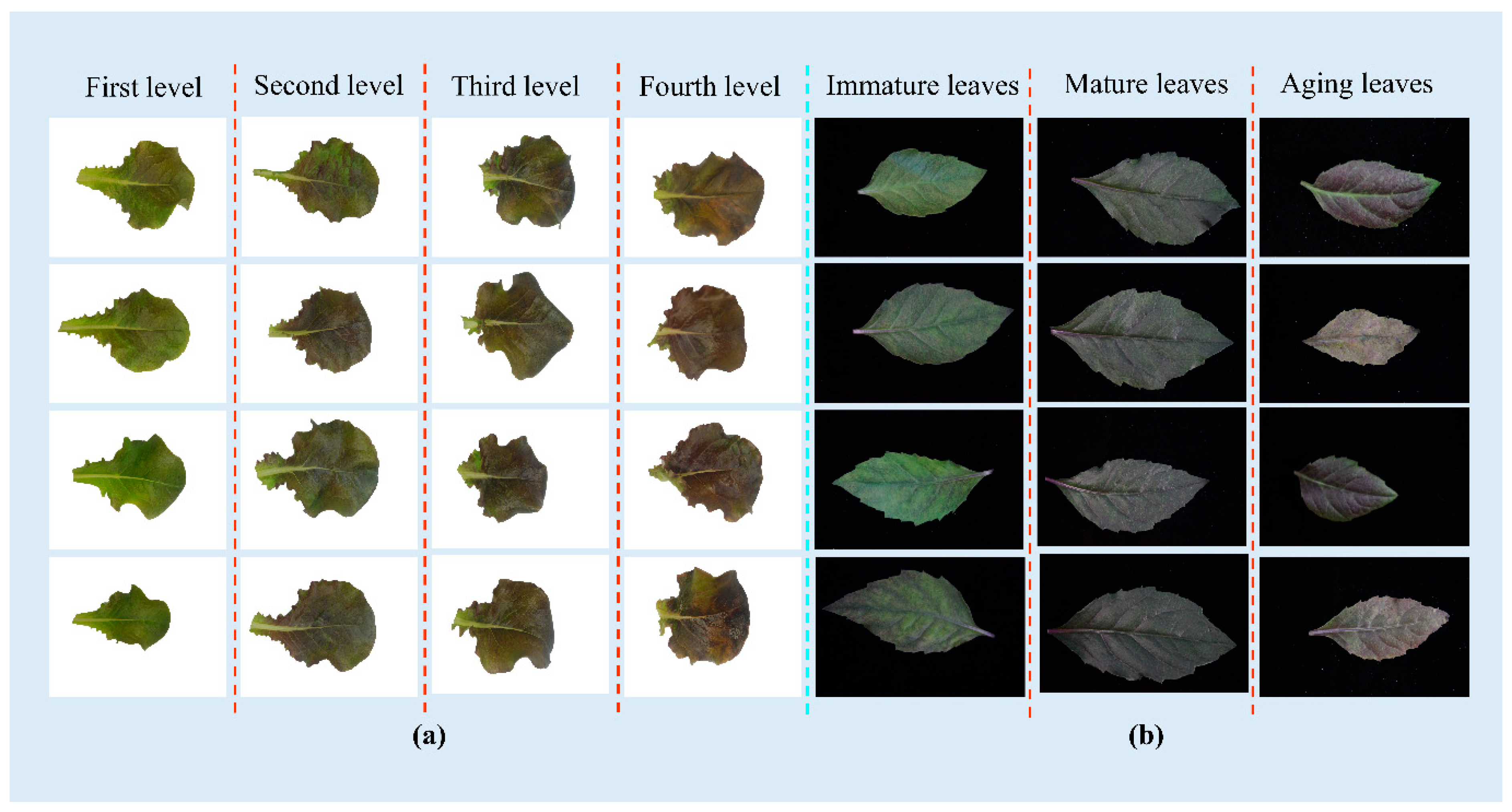
Sony ILCE-5000L/A5000 mirrorless camera was used to obtain visible-light images of leaves. Fixing the camera’s parameters and height for acquiring. The available leaves (avoiding the bottom and top 2–3 leaves) were cut and tiled on white paper. As a result, a total of 1113 images were acquired, of which the four categories each contained 241,334,298,240 images. Figure 2a shows some samples of our original dataset.

Besides, in order to evaluate the generalization performance of the model on other datasets, we selected the Gynura bicolor DC (G. bicolor) leaves in three growth periods [17] to further evaluate the model. This dataset involves three growth periods leaves of immature, mature, and aging collected in our previous work. Some samples of G. bicolor leaves are shown in Figure 2b.

3.1.2. Image Preprocessing

Data augmentation is an effective way to improve the robustness of the model, and the easiest way to solve the problem of imbalance between classes. In our work, mirror rotation, image sharping, salt and pepper noise were chosen to increase the sample size. These methods will not change the color and texture of samples, thus they will not introduce too much noise and blur the differences between adjacent categories. Besides, we controlled the number of augmented images in each category to achieve a balanced state between classes.

3.2. The Architecture of Tr-CNN

3.2.1. Overall Structure of Tr-CNN

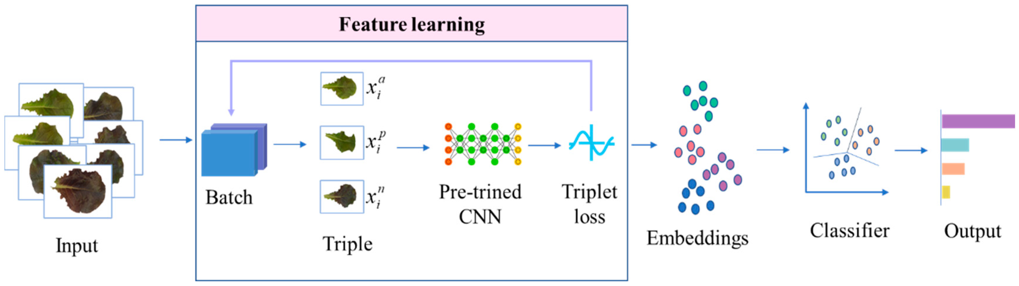
The overall architecture is shown in Figure 3. First, feature embeddings are extracted based on the network combined triplet loss function and CNN. The embeddings are then classified using SVM. Several modules included in the network are defined as follows:

• Baseline

Efficient learning of image features is a key step of classification task. Several classical networks (ResNet, NasNet, VGGNet, InceptionV3) were used as baseline to extract features. Furthermore, in order to solve the problem of slow convergence and are prone to get stuck in local optima of triplet loss, we chose the pre-trained CNN model (remove the fully connected layer) on ImageNet as the benchmark and compared their performance to determine the best model on our dataset.

2.

Dimensionality reduction

The dimensionality reduction of high-dimensional features can extract effective information and discard useless data, which is significant for the efficient execution of classification tasks. The commonly used method of dimensionality reduction is principal component analysis (PCA). It treats the data as a whole to find the optimal linear projection when the mean square error is the smallest, which may cause data mixing and decrease the classification accuracy. In this work, a fully connected layer was added after the convolutional layer to increase the nonlinear expression of the model. We explored the number of neurons in the fully connected layer through experiments to find the optimal dimensionality reduction.

3.

Classification

Support Vector Machine (SVM) was chosen as classifier in this experiment. Under the condition of high dimension and small sample size, SVM classifier has more advantages in resisting overfitting and outliers. SVM can use the kernel function to map embeddings to high-dimensional space, which is widely used in image classification. Multiple combinations of two kernel functions (Rbf and Liner), and multiple sets of optimal penalty parameters and kernel function parameters were tried in the experiment. Therefore, each group of data obtains its optimal parameter combination through training.

3.2.2. Feature Mapping Based on Triplet Loss Function

In this paper, Tr-CNN was built to solve the problem of small inter-class variance and large intra-class variance for stress levels. The execution of this module depends on the triplet loss function, which can optimize the feature mapping distance between different categories of images in high dimensional feature space. The goal of the framework is to learn a metric embedding function f(x) that can map the input image to a feature space: R^I → R^F. In this feature space, the images from the same category are “pulled closer”, and from the different categories are “pushed away”. The network input is a triple <a, p, n>, where a (anchor) represents a randomly selected anchor, p (positive) is a sample of the same category as a, and n (negative) indicates a sample of a different category from a. The three inputs share network parameters. To meet the requirements of image feature mapping, triples should satisfy the following conditional expressions:

$$\begin{array}{l}{\Vert f(x_i^a)-f(x_i^p)\Vert }_2^2+\alpha <{\Vert f(x_i^a)-f(x_i^n)\Vert }_2^2\\ \forall (f(x_i^a),f(x_i^p),f(x_i^a),)\in T\end{array}$$

(1)

In formula (1), T represents the set of all triples in a batch and $x_i^a$ is a randomly selected anchor. $x_i^p$ represents the sample of the same class as the anchor, and $x_i^n$ represents the sample of a different category from the anchor. α means the threshold for constraining the distance between positive and negative pairs. f(.) indicates the CNN network as a feature extractor. ${\Vert f(x_i^{})-f(x_i^{})\Vert }_2^2$ represents the Euclidean distance between two embedded features normalized by L₂. According to formula (1), the triplet loss function can be written as formula (2):

$$L={{\displaystyle \sum _i^N\left[{\Vert f(x_i^a)-f(x_i^p)\Vert }_2^2-{\Vert f(x_i^a)-f(x_i^n)\Vert }_2^2+\alpha \right]}}_{+}$$

(2)

where N represents the batch size participating in the batch training. The function makes the distance between sample pairs (a, p) less than the distance between (a, n), while the distance gap is greater than the margin.

Previous studies have shown that slow convergence and overfitting usually occurred in the feature extraction network based on triplet loss function [40]. Therefore, we migrated the CNN model pre-trained on ImageNet as the baseline network.

3.2.3. Triplet Selection for Effective Training

When constructing triples, not all of them are helpful for model training. Exhaustive training of all triples will bring greater computational pressure, so the choice of triples is very crucial. Semi-hard triple selection method is chosen in this work [41]. That is, the samples meet:

$${\Vert f(x_i^a)-f(x_i^p)\Vert }_2^2<{\Vert f(x_i^a)-f(x_i^n)\Vert }_2^2<{\Vert f(x_i^a)-f(x_i^p)\Vert }_2^2+\alpha$$

(3)

The meaning of each element in formula (3) is the same as formula (2).

For a training set $D={\left\{(x_i,y_i)\right\}}_{k=1}^N$ with N samples, the feature extraction process is shown in Algorithm 1:

Algorithm 1 Triplet-sampling CNN     Procedure 1 Feature Extraction

Input: Training set $D={\left\{(x_i,y_i)\right\}}_{k=1}^N$, margin α = 0.1.     Output: Feature learning model f(x).     1: Parameters from pre-trained CNN model as initialization values;     2: for each iteration do     3:        Generate triplets according to Equation (3)     4:        Map sample xi to Euclidean space through feature expression f(x)     5:        Calculate the Euclidean distance between sample pairs     6:        Calculate triplet loss according to Equation (2)     7:        Backpropagation and update parameters     8: end for

3.3. Experiment Settings

3.3.1. Experimental Environment and Settings

The experiment was conducted on a Windows 10 64-bit PC equipped with Intel(R) Xeon(R) CPU @ 2.20 GHz processor and 32 GB-RAM. Our program runs on NVIDIA GeForce GTX 1080 Ti GPU. The CNN model is implemented on the Keras framework, which is an advanced neural network API, written with python and can run on Tensorflow, CNTK or Theano.

The basic parameter settings of the model are shown in

Table 1. Hyperparameters in Tr-CNN training.

Parameter	Value
Optimizer	Adam
Batch size	40
Epoch	50
Initial learning rate *	0.001
Momentum	0.9
Margin #	1.0

* Learning rate decreases by a factor of 1/5 every 20 epochs, alternately; ^# Margin represents the distance between the class pairs.

. Especially, the learning rate decreases by a factor of 1/5 every 20 epochs, alternately. Besides, the margin is used to control the distance difference between sample pairs.

Different comparative experiments are performed to explore better parameter settings. Multiple excellent pre-trained models are used for feature extraction to find the optimal baseline. In addition, we have made many attempts on the dimension of the fully connected layer to find the law of the feature mapping dimension on the model.

3.3.2. Experimental Evaluation

In order to evaluate the effect of image feature mapping, the high-dimensional features outputted from CNN were reduced by PCA and then visualized on the two-dimensional plane. The mapping effect is evaluated by the visualization of the training set and test set.

In addition, confusion matrix, average precision, precision, recall and F1-score were used to evaluate the model classification effect. These indicators are described as follows: True positive (TP) means that the predicted value and actual value are both positive; False positive (FP) indicates the predicted value is positive, but the actual predicted value is negative; False negative (FN) means the predicted value is negative and the actual value is positive; True negative (TN) means the predicted value and actual value are both negative. The definitions can be expressed based on Formulas (4)–(7):

$$\mathrm{Pr}ecision=\frac{TP}{TP+FP}$$

(4)

$$\mathrm{Re}call=\frac{TP}{TP+FN}$$

(5)

$$Accuracy=\frac{TP+TN}{TP+TN+FP+FN}$$

(6)

$$F1=\frac{2TP}{2TP+FP+FN}$$

(7)

4. Results

In this section, we first analyzed the results using different CNN models to determine the optimal baseline for our dataset. The embeddings based on different pre-trained CNN models are visualized to evaluate the mapping effects on the training set and test set. Then, the classification effect of embeddings on SVM and the direct results of the corresponding pre-trained CNN model are compared and analyzed in detail. After determining the optimal baseline, we further discussed the feature mapping dimension of the model.

4.1. Feature Mapping Effect

In our framework, CNN is used to learn the feature mapping of the image set. Meanwhile, the feature distribution is optimized by the triplet loss function. At present, many classic models have been proposed and shown excellent performance in various tasks. But it’s important to choose a suitable model for a specific task. Therefore, the outstanding models on classification tasks VGGNet, InceptionV3, ResNet and NasNet were experimented to find the model suitable for our tasks. In addition, since training a stable model requires sufficient image set support, so we chose models pre-trained on ImageNet as the baseline.

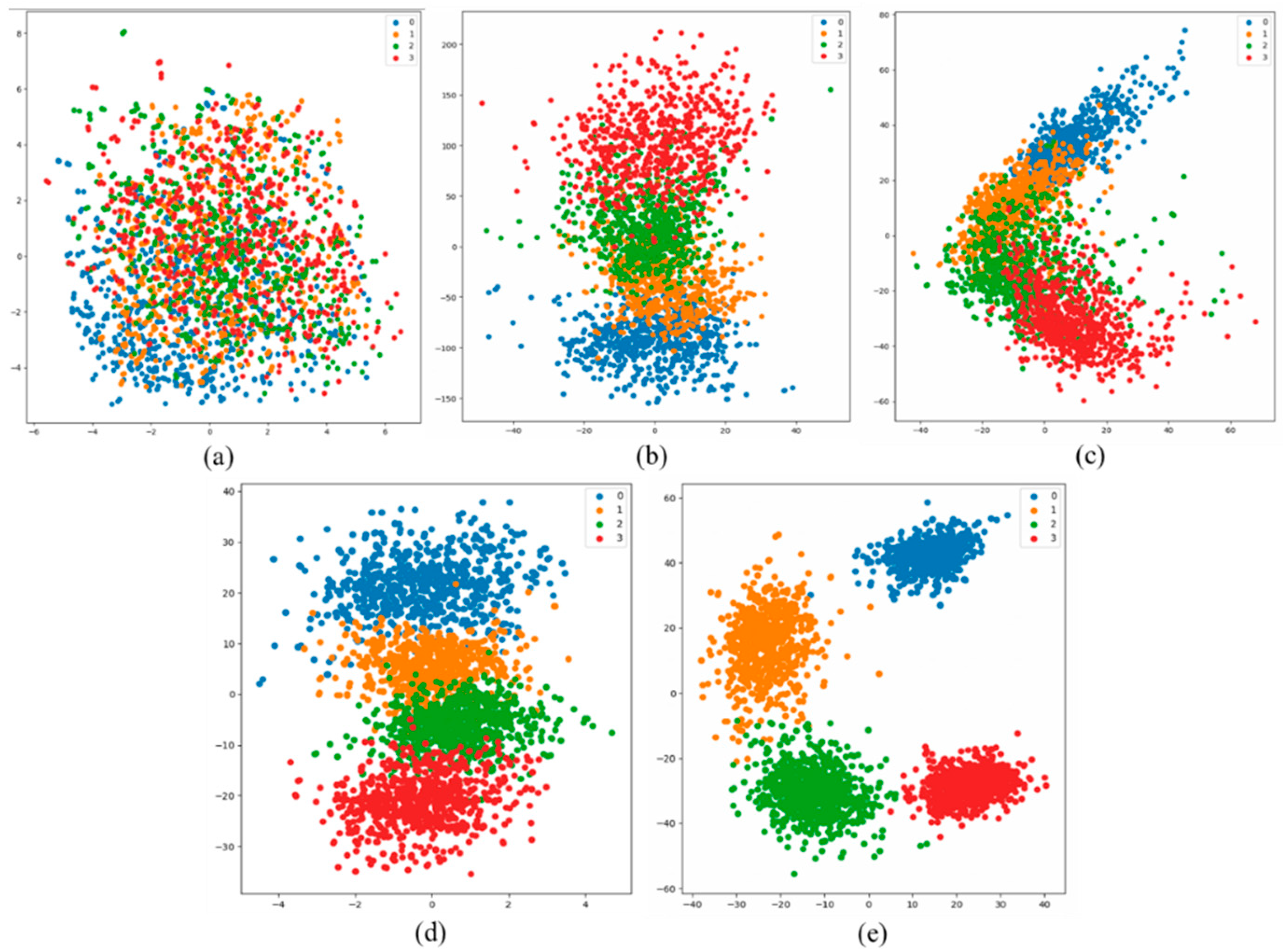
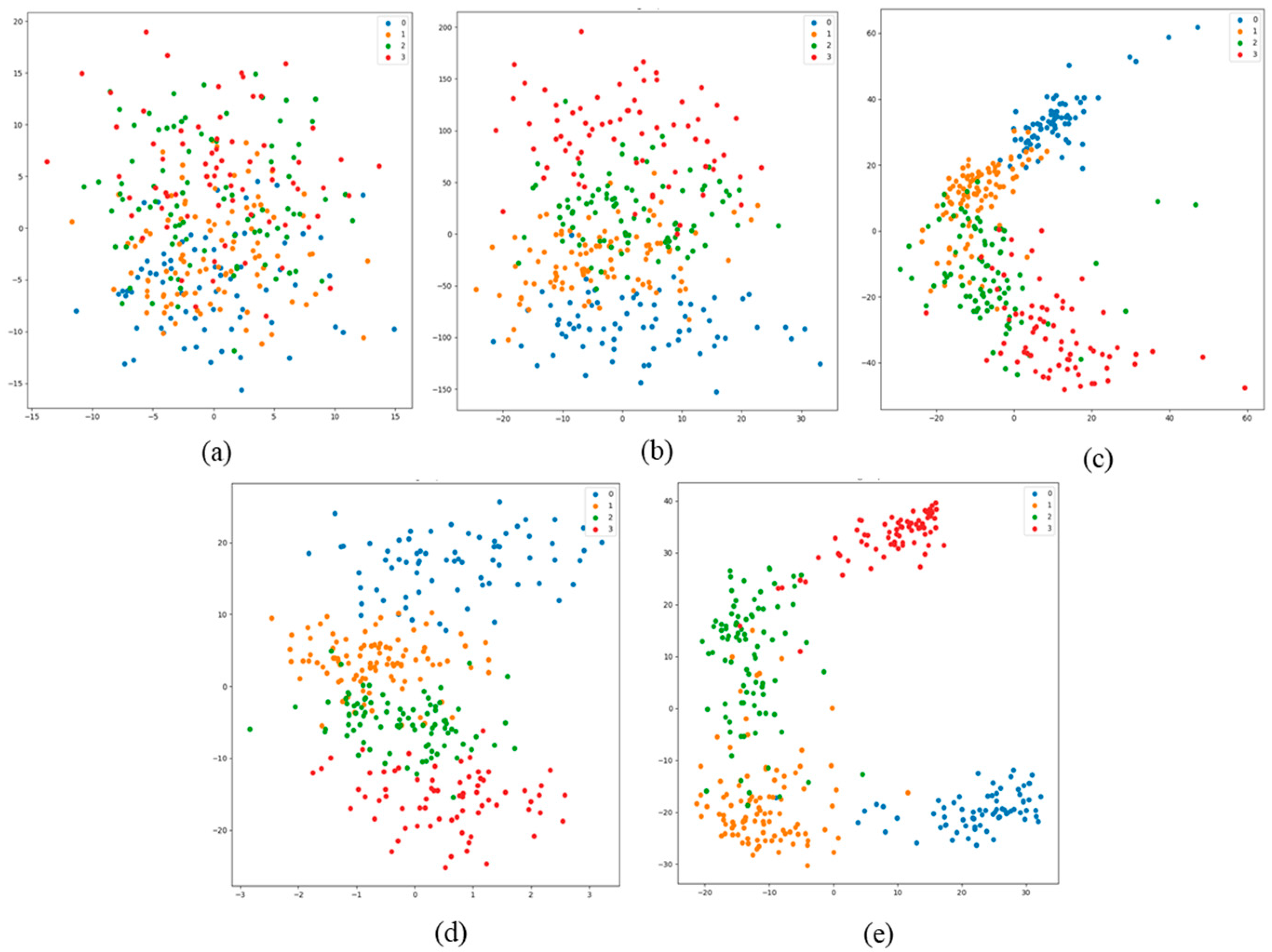
The training embeddings extracted by different baselines are visualized on a 2D surface. Figure 4a shows the feature distribution of the dataset before training. From the distribution, the features of different classes overlap severely except the first category. This reflects the phenomenon that the confusion in inter-class features and the scatter in intra-class. From b–e of Figure 4, after optimization of different models, image feature distribution presents different degrees of improvement. This proves the effectiveness of the proposed framework in solving the problem of image set mapping in fine-grained classification. Besides, the feature mapping results show obvious differences in different baseline models. From ResNet, NasNet and VGGNet, the embeddings between two adjacent classes still occur partially overlap. For the embeddings from inceptionv3, not only do adjacent classes have good spatial separability, but the feature aggregation effect within the class is better. Figure 5 shows the mapping effect of different models on the test set. Similar to the effect on the training set, InceptionV3 achieved the best mapping effect on the test set. In addition, the four models after training show the same visualization effects on the training set and the test set, which fully proves that there were no over-fittings during training.

4.2. Classification Performance Evaluation

After the network training, the image set is mapped to 512-dimensional embeddings. Then they were sent to SVM for classification. For evaluating the effectiveness of our proposed framework, the classic CNN models pre-trained on ImageNet (InceptionV3, ResNet-50, NasNet-Mobile and VGG-16) were also used for grading tasks. Classification results are presented in

Table 2. Classification results of all the applied models.

Method	Accuracy (%)	Precision	Recall	F1-Score
InceptionV3-based	91.5	0.923	0.920	0.915
NasNet-based	86.3	0.872	0.869	0.864
ResNet-based	83.3	0.838	0.842	0.832
VGGNet-based	84.5	0.860	0.850	0.847
InceptionV3	89.4	0.899	0.898	0.894
NasNet	74.5	0.765	0.768	0.725
ResNet	86.9	0.875	0.879	0.868
VGGNet	70.2	0.734	0.734	0.680

.

In Table 2, the first four rows represent the classification results from Tr-CNN based on different CNN baselines, while the last four rows list the results based on different pre-trained CNN models. Tr-CNN with InceptionV3 as baseline obtained the best results on all the metrics. Except for ResNet, Tr-CNN with different baselines have achieved better results than their corresponding original models (such as InceptionV3-based and InceptionV3). The contrast especially striking between NasNet-based and NasNet, VGGNet-based and VGG-16. These prove the validity of the framework we designed. In addition, on our data set, both inceptionV3 and inceptionV3-based performed very well, while the classic ResNet did not achieve the desired results.

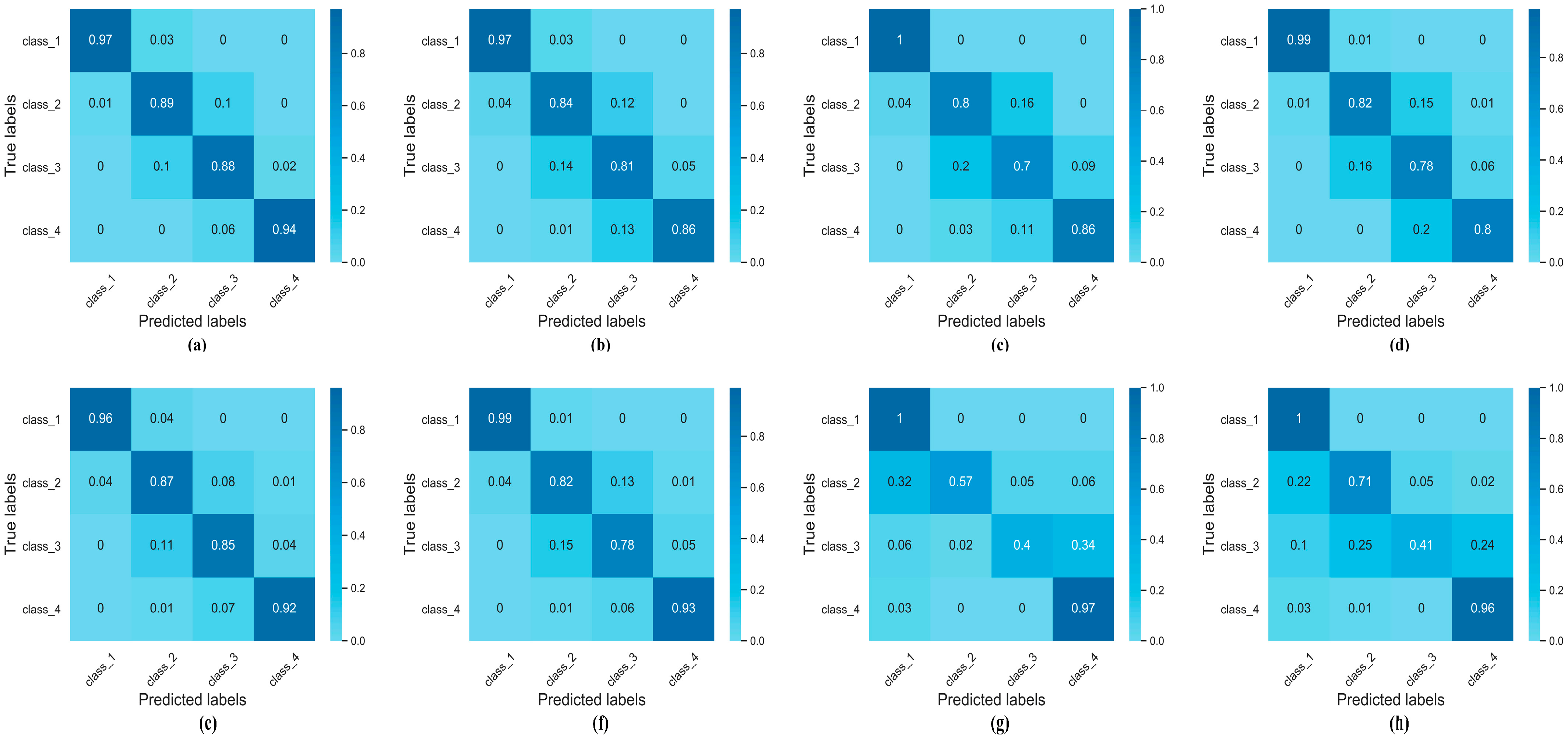
Confusion matrix (as is shown in Figure 6) can describe the individual classification rate by comparing the predicted category (abscissa) and the actual category (ordinate). Based on the numerical distribution of the confusion, the first and fourth classes show a better classification effect (averaged at 98.9% and 90.5%). The leaves under extremely weak or strong light conditions have obvious separability. Conversely, there are many misclassifications between the second and third categories, resulting in a lower individual classification rate (averaged at79% and 70.1%). This is primarily related to small differences between these two categories. ResNet, ResNet-based and VGGNet, VGG-based have poor classification effects on the second and third categories. This could be attributed to the two models that have a large number of parameters is difficult to achieve better training results under limited training data. In contrast, InceptionV3, InceptionV3-based, NasNet, and NasNet-based show better performance in the four categories. Among them, InceptionV3-based performed best, especially in the second and third categories. Overall, Tr-CNN based on different baselines shows better results than their baseline model in the second and third categories, which indicates the advantages of Tr-CNN in solving the fine-grained image problems.

4.3. Determination of Embeddings Dimensions

Through the above experiment, InceptionV3 was finally determined as the baseline of Tr-CNN for feature embedding. Besides, the initial dimensions of feature embeddings were set as 512 based on previous works [42,43]. In this part, experiments were performed on different dimensions to explore the impact of the feature mapping dimension on the classification effect and find the dimension suitable for our data set.

Table 3. Results under different dimensions of embeddings.

Dimensions	Accuracy (%)	Precision	Recall	F1-Score
1	90.9	0.916	0.916	0.900
4	91.2	0.917	0.917	0.911
16	92.3	0.930	0.928	0.923
64	92.4	0.930	0.930	0.924
128	91.5	0.922	0.921	0.915
256	90.3	0.910	0.911	0.902
512	91.5	0.923	0.920	0.915
1024	89.4	0.901	0.902	0.893
2048	89.1	0.920	0.897	0.892
4092	86.9	0.878	0.875	0.870
8192	81.2	0.825	0.818	0.813

lists the classification results under feature mapping of different dimensions.

In Table 3, in order to evaluate the classification effect in different dimensions stably, we take the weighted average of the three results as the final evaluation index. No significant difference was observed when the feature embedding is mapped below 512 dimensions. This shows that the lower mapping dimension will not harm the classification effect. As the dimensionality increases, the results show a clear downward trend. This may be due to some redundant information have been introduced when the embedding dimension is too large.

4.4. Generalization Experiment

In order to test the generalization ability of the Tr-CNN on other datasets, a growth period classification dataset was used to train and test on Tr-CNN and its related models. This dataset was created in our previous work, which includes a leaf image set of Gynura bicolor DC in three growth periods (some samples are shown in Figure 2b). It’s similar to our task due to the small difference between the three categories. The test results of all the models are listed in

Table 4. Classification results of all the applied models on the growth period classification dataset.

Method	Accuracy (%)	Precision	Recall	F1-Score
InceptionV3-based	91.7	0.918	0.917	0.916
NasNet-based	85.3	0.853	0.853	0.852
ResNet-based	78.2	0.800	0.782	0.781
VGGNet-based	90.4	0.911	0.904	0.902
InceptionV3	89.1	0.891	0.891	0.889
NasNet	89.1	0.891	0.891	0.890
ResNet	70.5	0.740	0.705	0.688
VGGNet	71.8	0.744	0.718	0.714

. The results presented in this paper are different from the original reference due to the difference in dataset augmentation and division, and the use of pre-trained models.

Except for NasNet, all the models have been improved compared to the corresponding baseline, especially VGGNet-based. The dataset size is similar to the light intensity classification dataset, so neither ResNet nor VGGNet achieves ideal results at this magnitude. Nevertheless, with the help of triplet loss to solve small samples, Tr-CNN based on ResNet and VGGNet has been greatly improved over the baseline model. InceptionV3 has achieved the best results on both datasets, proving its advantages in fine-grained classification tasks with limited sample size.

5. Discussion

The following aspects highlighted through the above experiments:

• Tr-CNN has been associated with satisfactory results.

Triplet loss function was introduced to realize the “separation” of features between classes and the “aggregation” within classes. The pre-trained model solves the problem of slow convergence and over-fitting. Besides, the framework uses SVM as a classifier. In the past, the main problem based on SVM classification is feature selection and extraction, while our framework solves the problem of single feature input of SVM.

2.

The classic CNN model will show huge differences when processing different datasets.

The classic CNN models we selected performed well on other tasks [44,45] but showed huge differences in our datasets. All the classic models have their specific structure and depth [46] and therefore apply to different scenarios. For example, large model architectures have better expressiveness and generalization ability, but they usually need huge data to achieve full learning, while some simplified model architectures can converge faster for simple tasks with small data volume. Therefore, different model architectures differ in their ability to adapt to different scenarios.

3.

The choice of the baseline is important for Tr-CNN.

Tr-CNN shows different increments on different baseline models. When solving the task of light stress classification, NasNet-based and VGGNet-based increase significantly, while ResNet-based is not improved on the basis of the baseline. Therefore, not only do different model architectures (depth, breadth, and number of parameters, etc.) have certain applicability to specific dataset, but also each submodule in the intact model (such as convolution module, fully connected module, classifier module, and loss function, etc.) has strong matching.

4.

Tr-CNN has a conspicuous advantage to deal with small inter-class variance in fine-grained image classification.

During the experiment, we also tried to use Tr-CNN to solve other classification problems, such as species classification based on leaves. However, not much progress has been made on such datasets. Tr-CNN focuses on optimizing image feature distribution with small intra-class variance and large inter-class variance. However, for the image sets with relatively obvious differences between classes, the common loss function such as cross-entropy loss has a simpler calculation process and faster convergence, which usually achieve better results.

5.

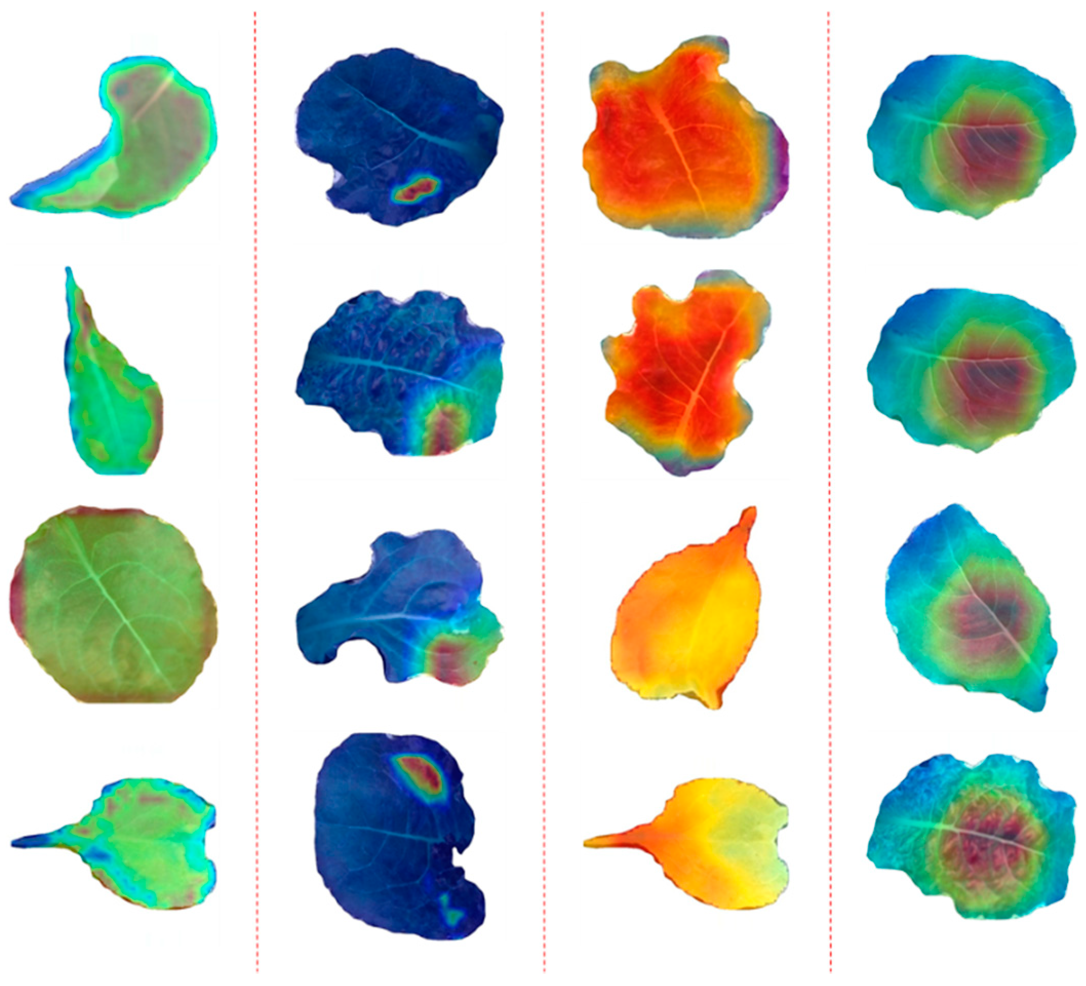
Many characteristics of leaves contribute to the grading of light intensity stress.

In our task, the texture, vein, edges, shapes, colors, and other hidden features of the leaves make the leaves separable between different levels of light intensity, but the “black box” nature of the network makes this mechanism difficult to quantify. Class Activation Map (CAM) [47] can be used to qualitatively express the contribution of features in the network in the form of heat map. In Figure 7, this contribution of different types of features is visualized by using CAM. The four columns from left to right respectively show the edge, local features such as sunburn parts, overall features such as color, and leaf vein. In addition, it is undeniable that the network can learn some hidden features that are difficult to explain, which is the potential of deep learning.

6. Conclusions

In this study, we used pre-trained CNN models as a baseline, triplet loss as loss function, and SVM as classifier to grade the light intensity stress of lettuce. This framework solves the problem of small inter-class features and large intra-class features in the classification task. Through multiple tests, inceptionV3 is determined as the baseline, and the dimension of embeddings is set as 64. Comparative and generalization experiments indicate that Tr-CNN is feasible in solving this kind of FGVC.

Although Tr-CNN showed good performance in light stress grading and growth period classification tasks, some work still needs to be improved in the future. We have proved the separability of light stress through the classification based on leaves. But the leaf is obtained by destructive means. Light stress classification based on plants or leaf segmentation methods should be studied to further serve practical applications. In addition, the optimization of triplet loss and the research of classifiers is all that needs to be done to further improve Tr-CNN.

References

- Fernández, V.; Eichert, T.; Del Río, V.; López-Casado, G.; Heredia-Guerrero, J.A.; Abadía, A.; Heredia, A.; Abadía, J. Leaf structural changes associated with iron deficiency chlorosis in field-grown pear and peach: Physiological implications. Plant Soil 2008, 311, 161. [Google Scholar] [CrossRef] [Green Version]
- Fu, W.; Li, P.; Wu, Y. Effects of different light intensities on chlorophyll fluorescence characteristics and yield in lettuce. Sci. Hortic. 2012, 135, 45–51. [Google Scholar] [CrossRef]
- Hao, X.; Jia, J.; Mi, J.; Yang, S.; Khattak, A.M.; Zheng, L.; Gao, W.; Wang, M. An optimization model of light intensity and nitrogen concentration coupled with yield and quality. Plant Growth Regul. 2020, 92, 319–331. [Google Scholar] [CrossRef]
- Kleinhenz, M.D.; Gazula, A.; Scheerens, J.C.; French, D.G. Variety, shading, and growth stage effects on pigment concentrations in lettuce grown under contrasting temperature regimens. HortTechnology 2003, 13, 677–683. [Google Scholar] [CrossRef] [Green Version]
- Reum, D.; Zhang, Q. Wavelet based multi-spectral image analysis of maize leaf chlorophyll content. Comput. Electron. Agric. 2007, 56, 60–71. [Google Scholar] [CrossRef]
- Chen, D.; Neumann, K.; Friedel, S.; Kilian, B.; Chen, M.; Altmann, T.; Klukas, C. Dissecting the phenotypic components of crop plant growth and drought responses based on high-throughput image analysis. Plant Cell 2014, 26, 4636–4655. [Google Scholar] [CrossRef] [Green Version]
- Esgario, J.G.; Krohling, R.A.; Ventura, J.A. Deep learning for classification and severity estimation of coffee leaf biotic stress. Comput. Electron. Agrc. 2020, 169, 105162. [Google Scholar] [CrossRef] [Green Version]
- Rahaman, M.M.; Ahsan, M.A.; Chen, M. Data-mining techniques for image-based plant phenotypic traits Identification and Classification. Sci. Rep. 2019, 9, 1–11. [Google Scholar] [CrossRef]
- Banerjee, K.; Krishnan, P. Normalized Sunlit Shaded Index (NSSI) for characterizing the moisture stress in wheat crop using classified thermal and visible images. Ecol. Indic. 2020, 110, 105947. [Google Scholar] [CrossRef]
- Bhugra, S.; Anupama, A.; Chaudhury, S.; Lall, B.; Chugh, A. Multi-modal Image Analysis for Plant Stress Phenotyping. In National Conference on Computer Vision, Pattern Recognition, Image Processing, and Graphics; Springer: Singapore, 2017; pp. 269–280. [Google Scholar]
- Amanda, R.; Kelsee, B.; Peter, M.C.; Babuali, A.; James, L.; Hughes, D.P. Deep learning for image-based cassava disease detection. Front Plant Sci. 2017, 8, 1852. [Google Scholar]
- Toda, Y.; Okura, F. How convolutional neural networks diagnose plant disease. Plant Phenomics 2019, 2019, 9237136. [Google Scholar] [CrossRef]
- Yang, W.; Yang, C.; Hao, Z.; Xie, C.; Li, M. Diagnosis of plant cold damage based on hyperspectral imaging and convolutional neural network. IEEE Access 2019, 7, 118239–118248. [Google Scholar] [CrossRef]
- Lu, J.; Tan, L.; Jiang, H. Review on Convolutional Neural Network (CNN) Applied to Plant Leaf Disease Classification. Agriculture 2021, 11, 707. [Google Scholar] [CrossRef]
- Ji, R.; Wen, L.; Zhang, L.; Du, D.; Wu, Y.; Zhao, C.; Liu, X.; Huang, F. Attention Convolutional Binary Neural Tree for Fine-Grained Visual Categorization. In Proceedings of the IEEE/CVF Conference on Computer Vision and Pattern Recognition, Virtual, 14–19 June 2020; pp. 10468–110477. [Google Scholar]
- Zhu, Y.; Sun, W.; Cao, X.; Wang, C.; Wu, D.; Yang, Y.; Ye, N. TA-CNN: Two-way attention models in deep convolutional neural network for plant recognition. Neurocomputing 2020, 365, 191–200. [Google Scholar] [CrossRef]
- Hao, X.; Jia, J.; Khattak, A.M.; Zhang, L.; Guo, X.; Gao, W.; Wang, M. Growing period classification of Gynura bicolor DC using GL-CNN. Comput. Electron. Agrc. 2020, 174, 105497. [Google Scholar] [CrossRef]
- Mohanty, S.P.; Hughes, D.P.; Salathé, M. Using deep learning for image-based plant disease detection. Front Plant Sci. 2016, 7, 1419. [Google Scholar] [CrossRef] [PubMed] [Green Version]
- Amara, J.; Bouaziz, B.; Algergawy, A. A Deep Learning-Based Approach for Banana Leaf Diseases Classification. Datenbanksysteme für Business, Technologie und Web (BTW 2017)-Workshopband. 2017. Available online: https://dl.gi.de/handle/20.500.12116/944 (accessed on 8 November 2021).
- Wang, Z.; Wang, X.; Wang, G. Learning fine-grained features via a CNN tree for large-scale classification. Neurocomputing 2018, 275, 1231–1240. [Google Scholar] [CrossRef] [Green Version]
- Karthik, R.; Hariharan, M.; Anand, S.; Mathikshara, P.; Johnson, A.; Menaka, R. Attention embedded residual CNN for disease detection in tomato leaves. Appl. Soft Comput. 2020, 86, 105933. [Google Scholar]
- Lu, H.; Cao, Z.; Xiao, Y.; Fang, Z.; Zhu, Y. Toward good practices for fine-grained maize cultivar identification with filter-specific convolutional activations. IEEE Trans. Autom. Sci. Eng. 2016, 15, 430–442. [Google Scholar] [CrossRef]
- Yu, Z.; Jiang, X.; Zhou, F.; Qin, J.; Ni, D.; Chen, S.; Lei, B.; Wang, T. Melanoma recognition in dermoscopy images via aggregated deep convolutional features. IEEE Trans. Biomed. Eng. 2018, 66, 1006–1016. [Google Scholar] [CrossRef]
- Dimitropoulos, K.; Barmpoutis, P.; Zioga, C.; Kamas, A.; Patsiaoura, K.; Grammalidis, N. Grading of invasive breast carcinoma through Grassmannian VLAD encoding. PLoS ONE 2017, 12, e0185110. [Google Scholar] [CrossRef] [Green Version]
- Hao, X.; Jia, J.; Guo, X.; Zhang, W.; Zheng, L.; Wang, M. MFC-CNN: An Automatic Grading Scheme for Light Stress Levels of Lettuce (Lactuca sativa L.) Leaves. Comput. Electron. Agrc. 2020, 179, 105847. [Google Scholar] [CrossRef]
- Trigueros, D.S.; Meng, L.; Hartnett, M. Enhancing convolutional neural networks for face recognition with occlusion maps and batch triplet loss. Image Vis. Comput. 2018, 79, 99–108. [Google Scholar] [CrossRef] [Green Version]
- Ming, Z.; Chazalon, J.; Luqman, M.M.; Visani, M.; Burie, J.C. Simple triplet loss based on intra/inter-class metric learning for face verification. In Proceedings of the 2017 IEEE International Conference on Computer Vision Workshops (ICCVW), Venice, Italy, 22–29 October 2017; pp. 1656–1664. [Google Scholar]
- Yu, T.; Yuan, J.; Fang, C.; Jin, H. Product quantization network for fast image retrieval. In Proceedings of the European Conference on Computer Vision (ECCV), Munich, Germany, 8–14 September 2018; pp. 186–201. [Google Scholar]
- Maergner, P.; Pondenkandath, V.; Alberti, M.; Liwicki, M.; Riesen, K.; Ingold, R.; Fischer, A. Combining graph edit distance and triplet networks for offline signature verification. Pattern Recognit. Lett. 2019, 125, 527–533. [Google Scholar] [CrossRef]
- Zhou, Q.; Zhong, B.; Lan, X.; Sun, G.; Zhang, Y.; Zhang, B.; Ji, R. Fine-grained spatial alignment model for person re-identification with focal triplet loss. IEEE Trans. Image Process. 2020, 29, 7578–7589. [Google Scholar] [CrossRef]
- Hadsell, R.; Chopra, S.; LeCun, Y. Dimensionality reduction by learning an invariant mapping. In Proceedings of the 2006 IEEE Computer Society Conference on Computer Vision and Pattern Recognition (CVPR’06), New York, NY, USA, 17–22 June 2006; pp. 1735–1742. [Google Scholar]
- Schroff, F.; Kalenichenko, D.; Philbin, J. FaceNet: A unified embedding for face recognition and clustering. In Proceedings of the 2015 IEEE Conference on Computer Vision and Pattern Recognition, IEEE Computer Society, Boston, MA, USA, 7–15 June 2015; pp. 815–823. [Google Scholar]
- Wen, Y.; Zhang, K.; Li, Z.; Qiao, Y. A discriminative feature learning approach for deep face recognition. In European Conference on Computer Vision; Springer: Cham, Switzerland, 2016; pp. 499–515. [Google Scholar]
- Chen, W.; Chen, X.; Zhang, J.; Huang, K. Beyond triplet loss: A deep quadruplet network for person re-identification. In Proceedings of the IEEE Conference on Computer Vision and Pattern Recognition, Honolulu, HI, USA, 21–26 July 2017; pp. 403–412. [Google Scholar]
- Zhang, Y.; Liu, D.; Zha, Z.J. Improving triplet-wise training of convolutional neural network for vehicle re-identification. In Proceedings of the 2017 IEEE International Conference on Multimedia and Expo (ICME), Hong Kong, China, 10–14 July 2017; pp. 1386–1391. [Google Scholar]
- Zhang, M.; Xu, G.; Chen, K.; Yan, M.; Sun, X. Triplet-based semantic relation learning for aerial remote sensing image change detection. IEEE Geosci. Remote Sens. Lett. 2018, 16, 266–270. [Google Scholar] [CrossRef]
- Tang, F.; Fu, X.; Cai, M.; Lu, Y.; Zeng, Y.; Zhong, S.; Lu, C. Multilevel Traffic State Detection in Traffic Surveillance System Using a Deep Residual Squeeze-and-Excitation Network and an Improved Triplet Loss. IEEE Access 2020, 8, 114460–114474. [Google Scholar] [CrossRef]
- Huang, C.; Li, Y.; Loy, C.C.; Tang, X. Deep imbalanced learning for face recognition and attribute prediction. IEEE Trans. Pattern Anal. 2019, 42, 2781–2794. [Google Scholar] [CrossRef] [Green Version]
- Lei, W.; Zhang, R.; Yang, Y.; Wang, R.; Zheng, W.S. Class-Center Involved Triplet Loss for Skin Disease Classification on Imbalanced Data. In Proceedings of the 2020 IEEE 17th International Symposium on Biomedical Imaging (ISBI), Iowa City, IA, USA, 3–7 April 2020; pp. 1–5. [Google Scholar]
- Yu, B.; Tao, D. Deep metric learning with tuplet margin loss. In Proceedings of the IEEE International Conference on Computer Vision, Seoul, Korea, 27 October–2 November 2019; pp. 6490–6499. [Google Scholar]
- Hermans, A.; Beyer, L.; Leibe, B. In defense of the triplet loss for person re-identification. arXiv 2017, arXiv:1703.07737. [Google Scholar]
- Ge, W. Deep metric learning with hierarchical triplet loss. In Proceedings of the European Conference on Computer Vision (ECCV), Munich, Germany, 8–14 September 2018; pp. 269–285. [Google Scholar]
- Zhang, J.; Lu, C.; Wang, J.; Yue, X.G.; Lim, S.J.; Al-Makhadmeh, Z.; Tolba, A. Training Convolutional Neural Networks with Multi-Size Images and Triplet Loss for Remote Sensing Scene Classification. Sensors 2020, 20, 1188. [Google Scholar] [CrossRef] [Green Version]
- Wu, Z.; Shen, C.; Van Den Hengel, A. Wider or deeper: Revisiting the resnet model for visual recognition. Pattern Recogn. 2019, 90, 119–133. [Google Scholar] [CrossRef] [Green Version]
- Zoph, B.; Vasudevan, V.; Shlens, J.; Le, Q.V. Learning transferable architectures for scalable image recognition. In Proceedings of the IEEE Conference on Computer Vision and Pattern Recognition, Salt Lake City, UT, USA, 18–22 June 2018; pp. 8697–8710. [Google Scholar]
- Zhao, S.; Peng, Y.; Liu, J.; Wu, S. Tomato Leaf Disease Diagnosis Based on Improved Convolution Neural Network by Attention Module. Agriculture 2021, 11, 651. [Google Scholar] [CrossRef]
- Selvaraju, R.R.; Cogswell, M.; Das, A.; Vedantam, R.; Parikh, D.; Batra, D. Grad-cam: Visual explanations from deep networks via gradient-based localization. In Proceedings of the IEEE International Conference on Computer Vision, Venice, Italy, 22–29 October 2017; pp. 618–626. [Google Scholar]