Toward Precision in Crop Yield Estimation Using Remote Sensing and Optimization Techniques


National Council for Scientific Research, Remote, Sensing Center, P.O. Box 11-8281, Beirut 11072260, Lebanon
Agriculture 2019, 9(3), 54; https://0-doi-org.brum.beds.ac.uk/10.3390/agriculture9030054
Submission received: 11 February 2019
/
Revised: 7 March 2019
/
Accepted: 8 March 2019
/
Published: 13 March 2019
(This article belongs to the Special Issue Precision Agriculture)
Abstract
:Many crop yield estimation techniques are being used, however the most effective one is based on using geospatial data and technologies such as remote sensing. However, the remote sensing data which are needed to estimate crop yield are insufficient most of the time due to many problems such as climate conditions (% of clouds), and low temporal resolution. There have been many attempts to solve the lack of data problem using very high temporal and very low spatial resolution images such as Modis. Although this type of image can compensate for the lack of data due to climate problems, they are only suitable for very large homogeneous crop fields. To compensate for the lack of high spatial resolution remote sensing images due to climate conditions, a new optimization model was created. Crop yield estimation is improved and its precision is increased based on the new model that includes the use of the energy balance equation. To verify the results of the crop yield estimation based on the new model, information from local farmers about their potato crop yields for the same year were collected. The comparison between the estimated crop yields and the actual production in different fields proves the efficiency of the new optimization model.
1. Introduction
Remote sensing has proved to be game changing for the agricultural sector, as it is one of the backbones of precision in agriculture [1]. In remote sensing, multispectral and hyperspectral satellite images play a major role in crop management; their ability to represent crop growth conditions on the spatial and temporal scale is remarkable. These images can describe the crop development, photosynthetic active radiation (PAR), biomass accumulation (Bio), leaf area index (LAI), Normalized Difference Vegetation Index (NDVI), Enhanced Vegetation Index (ENDVI), Perpendicular Crop Enhancement Index (PCEI), and many other indices [2,3]. In addition, climate data related to crops can also be extracted from satellite images such as albedo, surface temperature, and actual evapotranspiration [3,4,5].
Many approaches have been developed to translate remote sensing data into crop yields, and several reviews of such approaches exist [6,7,8]. Some of these approaches have faced several problems in estimating crop yield. One of these problems is the scarcity of remote sensing data suitable for use in crop management because of climatic conditions such as clouds [9,10]. Most of the time climatic conditions and low temporal resolution are the main obstacles that prevent decision makers from using remote sensing data to map crops and to estimate crop yields.
There are several articles that have used vegetation indices from one date image or multi-temporal images to estimate crop yield. Bastiaanssen and Ali [11] used Monteith’s model [12] in their research for the calculation of Absorbed Photosynthetically Active Radiation (APAR), Stanford’s model for determining light use efficiency, and the Surface Energy Balance Algorithm for Land (SEBAL) to describe the temporal and spatial variabilities in land wetness conditions. The results of this research showed that there were gaps between the estimated and the actual yield of about 1075 and 1246 kg/ha for wheat and rice due to a lack of enough remote sensing images that cover the crop growth season. In addition, SEBAL is a well-known energy based actual evapotranspiration model, but it is difficult to implement due to a priori intensive requirements of climate variables. In this paper, some of the techniques used by [11,12] to estimate crop yield are adapted for this research.
The hypothesis is that missing satellite data can be compensated by using new models. The available biomass data which can be calculated using a reliable energy balance model can be fitted to a specific curve representing the new model using an optimization algorithm.
In this research, the objectives were to estimate crop yield using another known energy balance model named Mapping EvapoTranspiration at high Resolution with Internalized Calibration (METRIC) [13]. This model is less dependent on climatic measurements to compute actual evapotranspiration.
The next step was to use satellite images such as Landsat 7 and 8 images with the METRIC model to estimate crop biomass. Later, in order to strengthen the performance and efficiency of the crop yield model, a new model was developed. The model is based on using an optimization algorithm to compensate for the absence of satellite data due to climatic conditions. Finally, it was proved that the new model is able to provide efficient results.
2. Materials and Methods
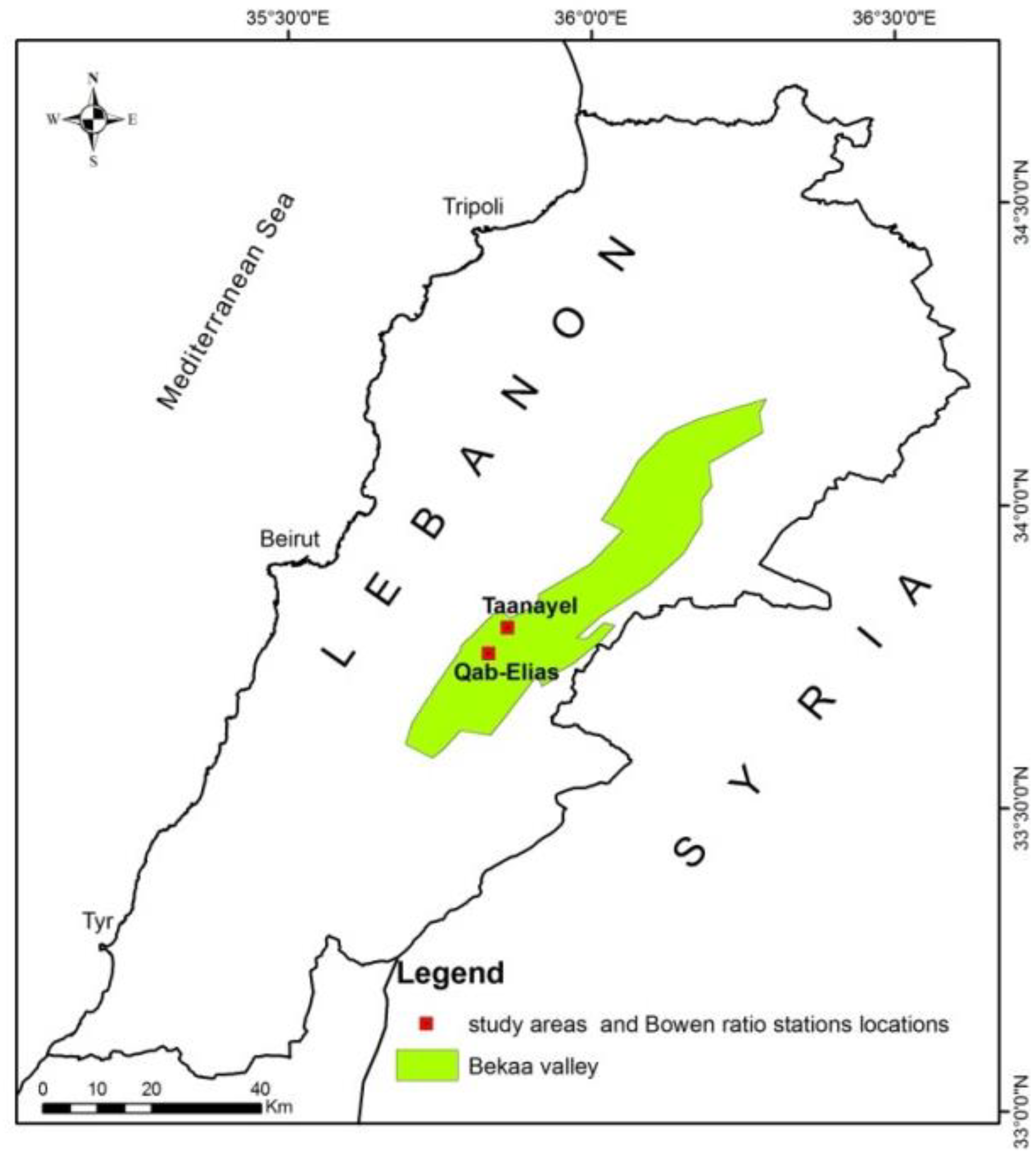
The study area is located in the largest agricultural plane in Lebanon, known as Bekaa valley. The plane has an area of more than 1000 km2, and the major crops in the valley are wheat, potato, and alfalfa. It is also important to note that two Bowen Ratio stations are installed in the area in order to measure the different climate parameters which are necessary for irrigation management, for mapping actual evapotranspiration, and for estimating crop yield (Figure 1).
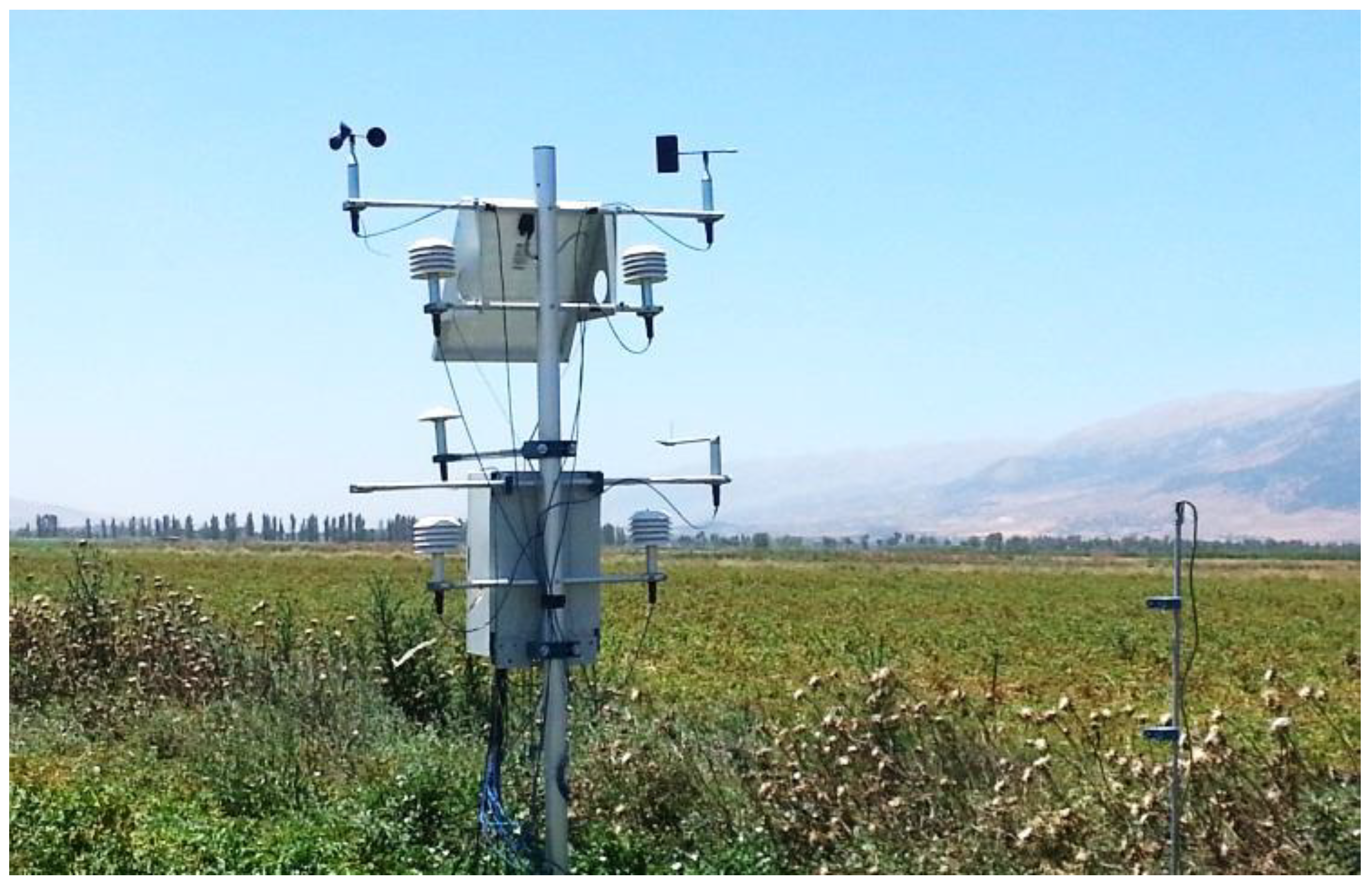
The two Bowen Ratio stations (Figure 2) are located in two different areas, one in an agricultural research institute in the middle of the plane, while the other is located south in a field owned by a potato chips manufacturer. The distance between both is more than 15 km. The two stations provide many valuable climate data such as net radiation, wind speed and direction, temperature at different elevations, humidity, global radiation, soil heat flux, and soil humidity. Increasing the number of Bowen ratio stations in the future could improve any model created based on the data of these stations. The images of Landsat 7 and 8 are used in this research and they can be downloaded free of charge from the United States Geological Survey (USGS) Web site [14].
In addition, these satellite images have thermal infrared bands with high spatial resolution (60 m compared to 1000 m for Modis Aqua and Terra satellites). The long wave infrared bands are used later in computing important parameters for crop yield estimation. Landsat images are collected between the date a specific crop was planted and the date the same crop is harvested. It is possible to collect all satellite images for the whole season if yield estimation is for more than one crop. Using both Landsat 7 and 8 improves the temporal resolution of image availability from 16 days to 8 days.
2.1. Estimating Crop Yield
Monteith model [12] is based on the photosynthetically active radiation (PAR) (0.4–0.7 m) which is part of the short wave solar radiation (0.3–3.0 m) that is absorbed by chlorophyll for photosynthesis in the plants.
Photosynthetically active radiation (PAR) is thus a fraction of the incoming solar radiation (Kinco). Then a fraction of PAR is absorbed by the plant for carbon assimilation.
Absorbed photosynthetically active radiation (APAR) in can be computed directly from PAR using the following equation
The factor f can be estimated using Normalized Differences Vegetation Index (NDVI) as is explained in [11]. Where
NDVI is the normalized difference vegetation index computed as the difference between near-infrared (NearIR) and red spectrums divided by their sum.
The accumulation of biomass is according to the Monteith model proportional to accumulated APAR.
where in (kg/m2) is the accumulated biomass in period t, ε is the light use efficiency in gram per mega joules (g MJ−1).
A more comprehensive global ecology model for computing net production was created by Field et al. [15] where they used the following equation for light use efficiency ε.
where ε′ is the maximum conversion element for above ground biomass when the environmental conditions are optimal, it is equal to 0.29 g/MJ for C3 crops [16]. W is a function of the effective fraction of the available soil moisture. The complete details for the calculation of W are explained later in the text.
T1 and T2 are two different heat functions, Topt (°C) which is the mean air temperature in the month with maximum leaf area index, and Tmon (°C) is the mean monthly air temperature. One can notice easily that T1 depends completely on Topt, which is in turn affected by canopy biomass. On the other hand, T2 depends on both Topt and Tmon.
2.2. Enhancement and Correction of the Images
Normally, Landsat “SLC-off” data refers to all Landsat 7 images collected after 31 May 2003, when Scan Line Corrector (SLC) failed. These products have data gaps, but are still useful and maintain the same radiometric and geometric corrections as data collected prior to the SLC failure. To fix this problem, a method created by Scaramuzza et al. [17] is used to fill gaps in one scene with data from another Landsat scene. In this method, linear transform is applied to the image with gaps to fix the problem based on the standard deviation and mean values of each band. The at-surface reflectance for the visible to short-wave is corrected on a band-by-band basis following Tasumi et al. method [18]. It works first on correcting images at sensor (Atmospheric correction) and then at surface correction.
Solar radiation reflected by the Earth’s surface to satellite sensors is modified by its interaction with the atmosphere. The objective of applying an atmospheric correction is to determine true surface reflectance values and to retrieve physical parameters of the Earth’s surface, including surface reflectance, by removing atmospheric effects [19]. Atmospheric correction for satellite images works as follow:
where: = top of atmosphere (TOA) reflectance, without correction for solar angle. Mp = Band-specific multiplicative rescaling factor, Ap = Band-specific additive rescaling factor, and Qcal = Quantized and calibrated standard product pixel values (DN). The constants Mp and Ap are extracted from the metadata file that comes with the image. While Qcal value is extracted from the image pixel values. To correct TOA for the sun angle, the following is applied
where is the corrected TOA reflectance, = local sun elevation angle. The next step is to correct with respect to at surface reflectance, which is done as follow:
where is at-satellite reflectance for band b, and is a band b specific given constant. and are narrowband transmittances for incoming solar radiation and for surface reflected shortwave radiation.
For more details on the atmospheric correction process one may refer to Tasumi et al.’s method [18].
2.3. Using METRIC
The computation of the evaporative fraction is based on using Equation (10), which in turn depends on the energy balance Equation (11):
where is the evaporative fraction unit less, H is the sensible heat flux in , latent heat flux in , Rn is the net radiation in , and G0 is the soil heat flux in . The equation can be solved using METRIC, which was developed by Allen et al. [13]. METRIC is a sort of “hybrid” between pure remotely sensed energy balance and weather-based evapotranspiration methods. Where energy balance is calculated from a satellite image which delivers spatial information that includes the available energy, and the sensible heat fluxes for a large area.
In this research, METRIC is used as part of the new model in order to calculate evaporative fraction and actual evapotranspiration. Both values are compared with the ones computed from the measurements collected by the Bowen Ratio stations.
METRIC’s foundation, principles and techniques are initially based on SEBAL [20,21]. However, METRIC differs from SEBAL in the way it works on solving Equation (10) by calculating each variable separately such that net radiation is calculated based on the following Equation (12)
where Rn is the net radiation in where RS↓ is the incoming shortwave radiation in , α is the surface albedo (dimensionless), RL↓ is the arriving longwave radiation in , RL↑ is the emitted longwave radiation in , and Eo is the surface thermal emissivity.
H is the sensible heat flux in , and are the air and surface temperatures in (°C), is the air density (kg m−3) and heat capacity of air, (Kj kg−1) are constants, and is the transfer resistance (s m−1), which depends on wind speed and surface characteristics.
where G0 is the soil heat flux in and LAI is the leaf area index unit. For more details about the above equations one may refer to the METRIC manual [22].
G0 = (0.05 + 0.10e−0.521LAI) Rn (LAI ≥ 0.5)
G0 = max (0.4 H, 0.15 Rn) (LAI < 0.5)
2.4. A New Optimization Technique
Since the estimation of crop yield depends on few satellite images there will be some periodic gaps between the date of planting and harvesting crops. For this reason, the information obtained from each image is used to create an optimization model to compensate for missing data.
Specific optimization models analyze observations from the real world, such as satellite images, in order to find a solution for data gaps. In this research these models were used to enhance data availability and to predict needed data in a specific information process known as biomass yield estimation. The optimization model finds global optimal solutions to fix the problem of data gaps with minimum error.
Normally, nonlinear curve-fitting (data-fitting) problems are solved using the least-squares method [23]. However, the data extracted from satellite images represent specific crop biomass which is considered a complex non polynomial (NP) type of problem and cannot be fitted to a simple linear equation. For this reason, there is a need for a more reliable method that can solve the problem and which can provide an optimal solution.
The objective is to fit a curve to the crop yield data using unconstrained nonlinear optimization algorithm such as Trust-Region Methods for Nonlinear Minimization [24]. Trust-region methods are efficient, and can solve easily ill-conditioned problems. The basic idea is to approximate a function F with a simpler function f, which reasonably reflects the behavior of function F in a neighborhood N around the point x. This neighborhood is the trust region, a trial step s is computed by minimizing over.
Biomass data were calculated using the Monteith model and satellite images with different acquisition dates. The data with acquisition dates were used in the optimization process to create the new biomass model. At the end, a new biomass yield equation was obtained (Equation (17)) which can compute the total accumulated biomass from the planting phase until crop maturity phase.
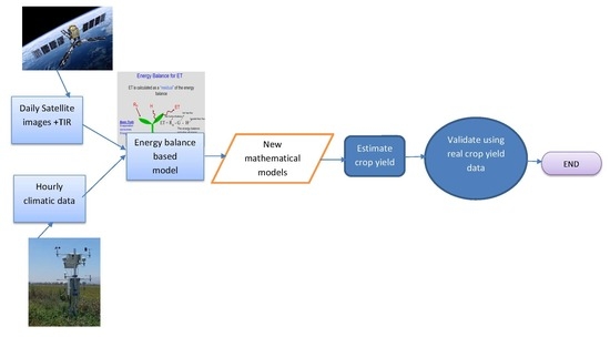
where NBio is the new total estimated biomass in kg/ha, Nd is the number of days, is the day i during the crop growth progress, and is the new optimization model that can be created from the estimated crop yield of the available Landsat image. The advantage of the new method is the ability to show the complete crop growth period even with the lack of a complete season of remote sensing images. Figure 3 shows in detail the steps needed to create the optimization model from few Landsat images.
3. Results
To conduct experiments it is required from the user to decide on the type of data, crop and the season length. The decision should be based on the availability of data and other information related to crop requirements. In case of any data gap the optimization model can be used improve the efficiency crop yield estimation process.
In this paper, potato crop yield, which has two different cycles, was estimated, but the majority of farmers plant potato at the end of winter/early spring and harvest in mid-summer. The potato leaves appears almost 20 days after seeding. Because the weather in Lebanon during winter and spring is mainly rainy and cloudy, it was very hard to get images during the months of March (the date potato was planted) and April. Seven satellite images were collected between the months of April, May, June, and July from the date of potato seeding (20 to 30 days after) and near the end of the growth stage (10 to 30 days before harvesting). Landsat 7 images were corrected and data gaps were filled using the methods explained above. Moreover, at-surface reflectance was calculated by applying atmospheric corrections at-satellite and at-surface reflectance.
3.1. Evaporative Fraction Calculation
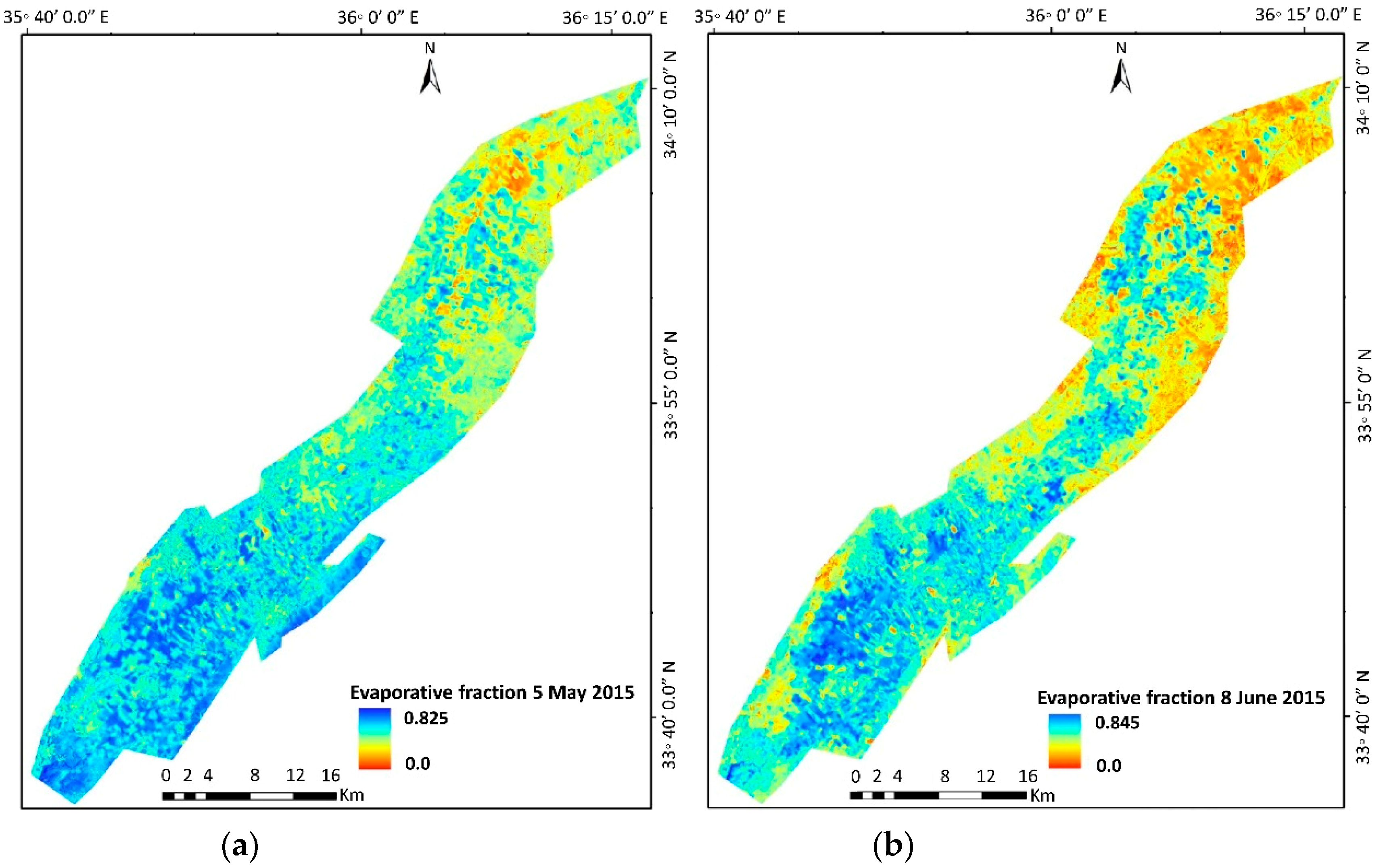
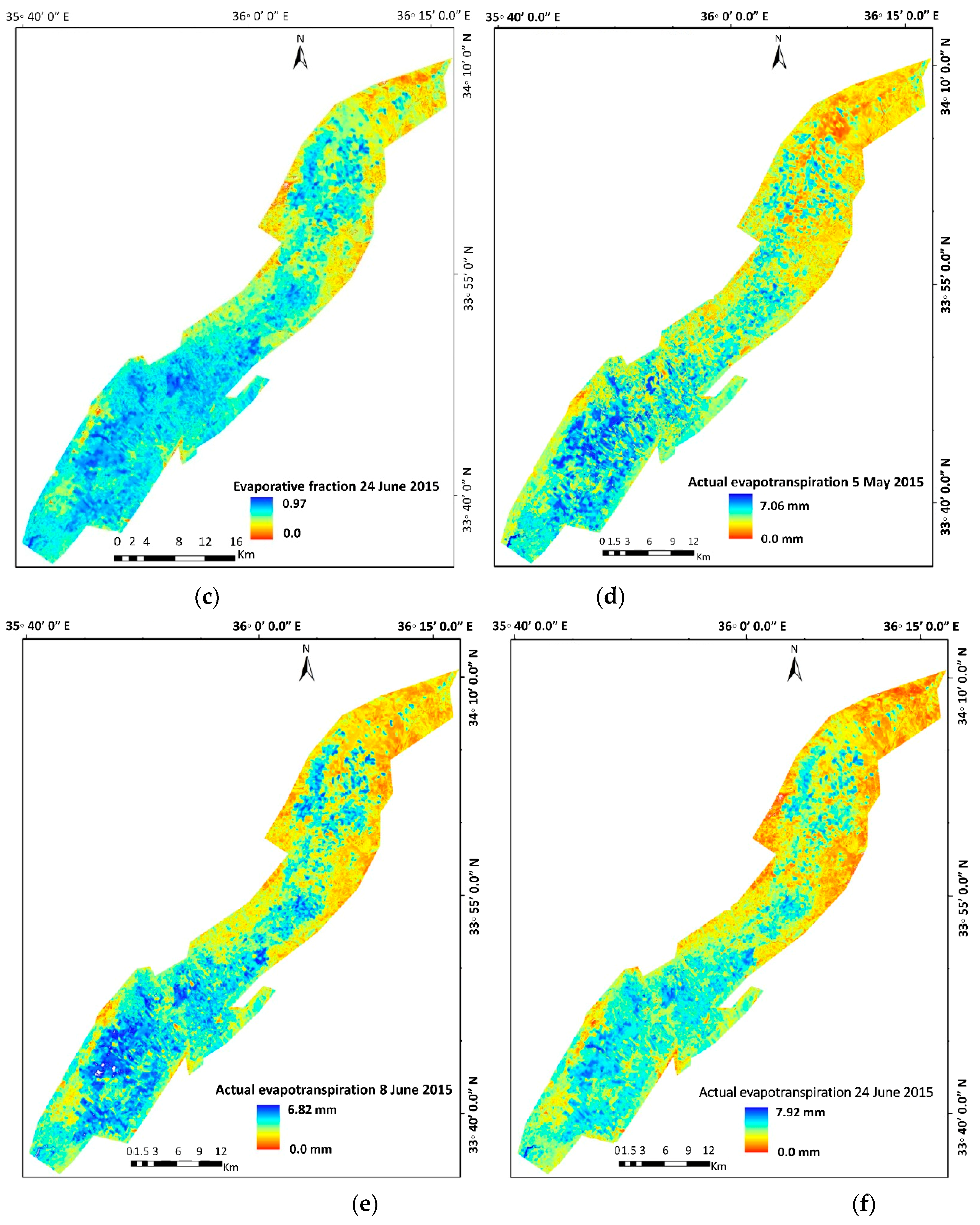
Evaporative fraction and actual evapotranspiration (Eta) maps are created using the METRIC model as explained in the method section. The map covers seven days in April, May, June and July.
The values of the evaporative fraction are less than 1, except in a few cases where net radiation was very large compared to sensible and soil heat fluxes () or when H was zero because air and surface temperature are equal or the difference was negligible.
To calibrate and to validate the accuracy of energy balance model (METRIC), some recorded climatic data from two Bowen Ratio stations were used to evaluate actual evapotranspiration and evaporative fraction estimated maps. In addition, records on irrigation use were collected from farmers in specific crop fields. These records were used to calibrate and validate METRIC products (Table 1). Figure 4a–f show the actual evapotranspiration maps and evaporative maps for a large area in Bekaa valley in the 5 May, 8 and 24 June 2015. The following data (Table 2) show the actual evapotranspiration values obtained from the Bowen Ratio stations (actual values) and the predicted values from the METRIC model for the month of June. The accuracy is computed based on the Mean Absolute Percentage Error (MAPE) [25].
Table 3 shows the computed evaporative fraction values for the local time between 9:00 and 14:00 on the 8 June 2015. The value of the predicted = 0.74 was computed by the METRIC model and then compared with the actual W computed from Bowen Ratio station data at time 11:00. The comparison shows that the absolute percentage error was 5%.
MAPE values were computed based on the actual evapotranspiration values from METRIC and the values of irrigation water volume for two days (8 and 24 June 2015). MAPE showed errors values that range between 11% and 18%. After investigating the issue, new facts were discovered. One of these facts is that the farmers usually do not adhere to the rules set by the water authorities in their area; they pump more water and normally record the fixed volume of water set by the authorities.
The estimated hourly evaporative fraction for the 24 June 2015 was also verified. The following data collected by Bowen Ratio station (Table 4) shows the different parameter values used by the energy balance equation. The value of the evaporative fraction W computed from Bowen station data (highlighted row in Table 4) is compared with the value of W computed by the METRIC model (value = 0.7). The result indicates that the absolute percentage error is 8%.
The results are promising, and they prove that W computed by the METRIC model are comparable to the ones obtained from the Bowen ratio data. In return, the estimated evaporative fraction can be used to solve the crop yield estimation problem.
3.2. Estimating Potato Crop Yield
To estimate potato yield, several Landsat 7 and 8 images were collected. However, the number of available images was not sufficient because a biomass model requires information about the complete crop growth stage. The problem can be solved if daily satellite images such as Modis are obtained, however the information extracted would be useless due to the coarse spatial resolution of this satellite (from 250 m to 1000 m), especially thermal long infrared image. So, the solution is to create an optimization model that can help to solve the issue of data gaps.
After creating the potato map, some statistical information related to biomass was extracted from seven processed satellite images. Although the seeding dates of spring potato are dynamic, the majority of farmers start the seeding process in the month of March, especially in the first two weeks. In addition, most of the farmers harvest potatoes in July.
Equation (18) is the result of fitting a curve to calculated biomass data from different remote sensing images based on using the Trust region algorithm. The parametric fitting of the given data involves finding coefficients (parameters) for one or more models that fit to data. The new biomass equation (Equation (19)) is based on using the new optimization model in Equation (18).
where Xdata is the day number from the beginning of the crop season to harvesting.
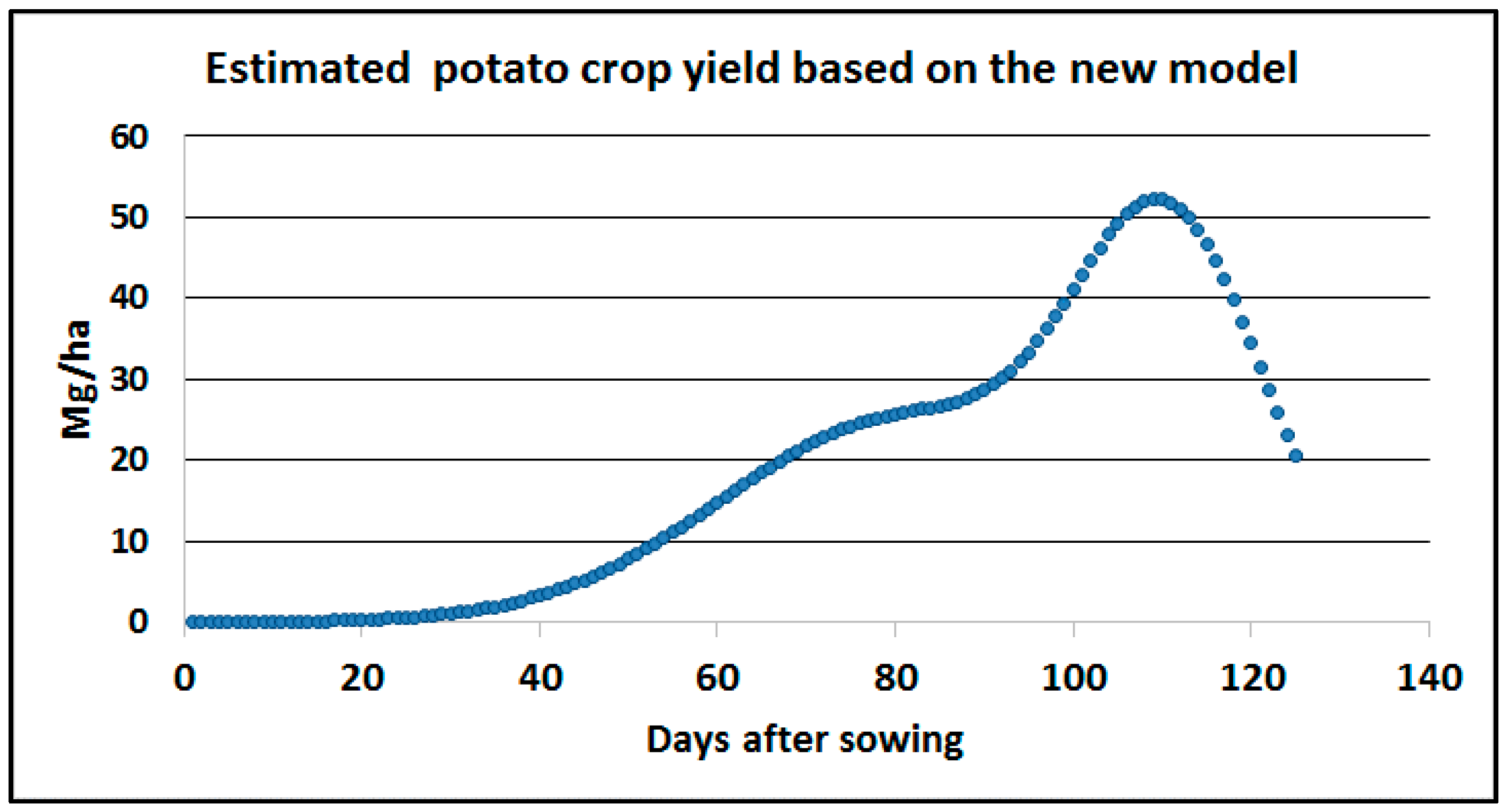
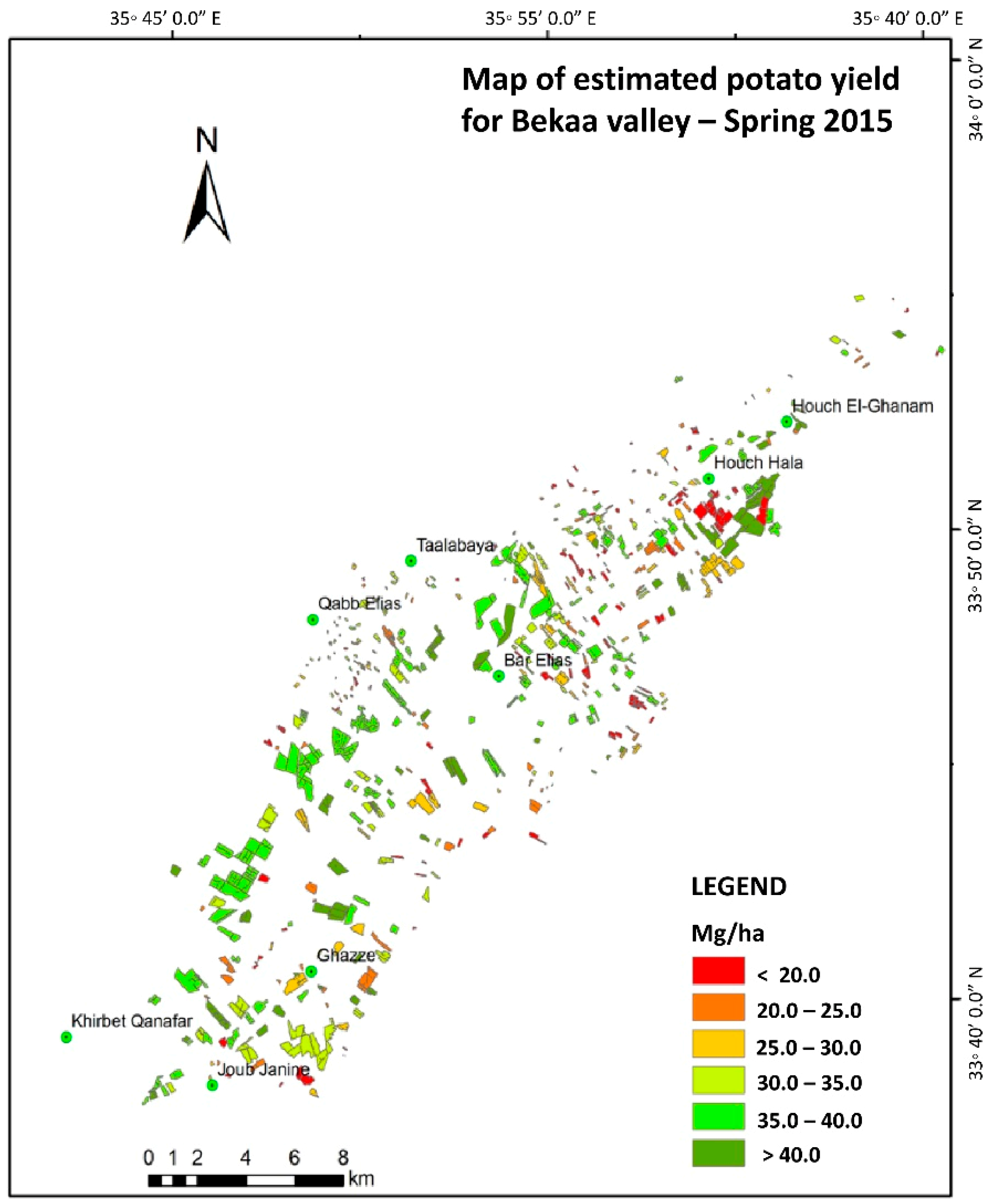
Figure 5 shows potato biomass growth progress after about three weeks from plantation and a few days before the end of the growth stage. The graph was created using the new yield model (Equation (19)). In addition, a map was created using the new crop yield method. Figure 6 shows the crop map, and estimated above ground crop biomass (for the whole season of potato spring 2015).
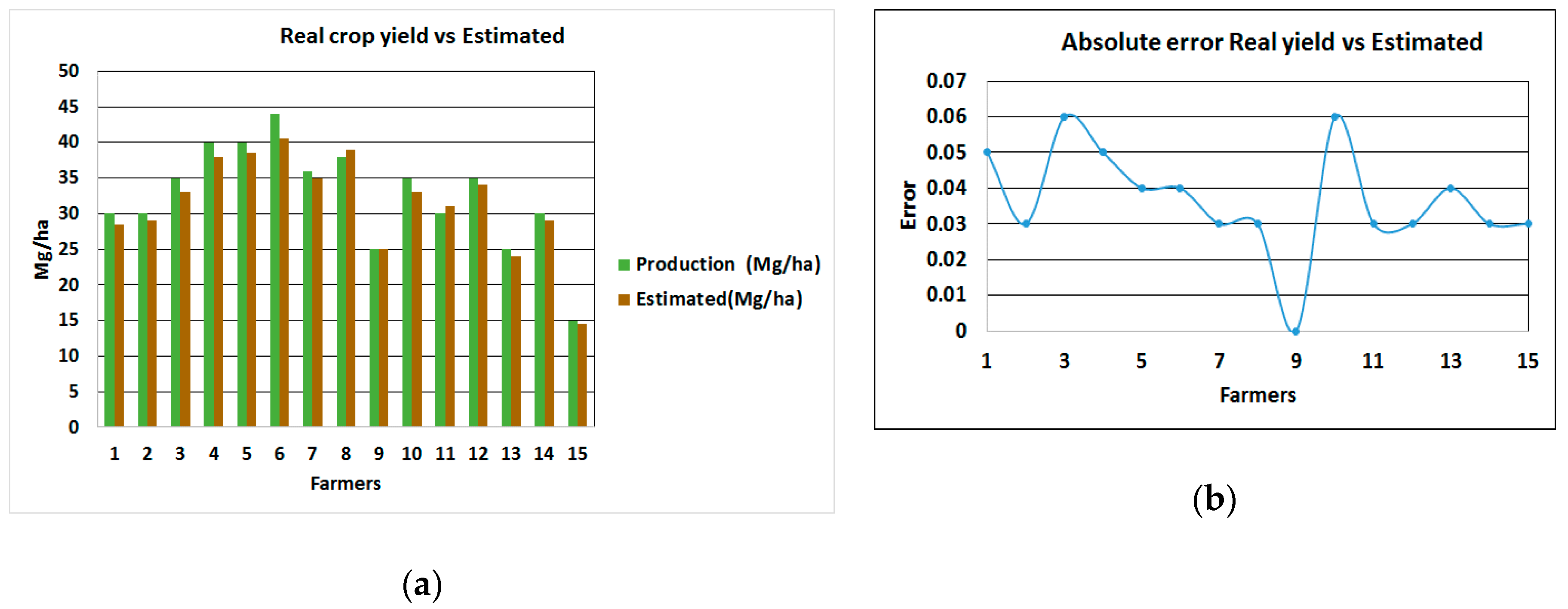
Data about potato crop yields were collected from 15 different farmers and they were used to verify the estimated results by the model. It is noticeable that there is close agreement between the estimated data in the map and the data collected from farmers (graph in Figure 7). Normally, a potato tuber is equal to up to 80% of the potato biomass [26].
MAPE is calculated for the estimated and real crop yield data and the error was less than 4%. Root-mean-square error (RMSE) was also used to estimate the accuracy of the results. RMSE is frequently used to measure the differences between values predicted by a model or an estimator and the values observed [27]. The value obtained for RMSE is 0.039, which is again an indication of high accuracy [28].
4. Conclusions
The lack of remote sensing data is no longer an obstacle for managers and decision makers in the agriculture sector. It is proved in this research that crop yield estimation can be improved if reliable model exists to help in overcoming all obstacles which hinder crop yield estimation processes. An optimization model created in this research is able to estimate crop yield by increasing remote sensing data availability. The optimization model was created by using a well-known algorithm, Trust-Region Methods for Nonlinear Minimization, that fits available data to an exponential equation. The experimental results proved the accuracy and reliability of the new model in estimating the crop yield in the case of missing remote sensing data (worst case scenario). The potato crop was used to prove the success of the objective of this research. It is planned to improve the optimization model by adding more components, crops, and seasons (agriculture years). This can help in managing many agriculture practices and tasks, and it can make different agriculture information available to decision makers in a highly precise way.
Funding
This research was funded by CEDRE program in Lebanon 2018–2020.
Acknowledgments
The author would like to thanks Lebanese CNRS for facilitating the achievement of this research.
Conflicts of Interest
The authors declare no conflict of interest.
References
- Anastasiou, E.; Balafoutis, A.; Darra, N.; Psiroukis, V.; Biniari, A.; Xanthopoulos, G.; Fountas, S. Satellite and Proximal Sensing to Estimate the Yield and Quality of Table Grapes. Agriculture 2018, 8, 94. [Google Scholar] [CrossRef]
- Da Silva, C.; Nannib, M.; Teodoroc, P.; Capristo Silva, G. Vegetation Indices for Discrimination of Soybean Areas: A New Approach. Agron. J. Abstr. Agron. Soils Environ. Qual. 2017, 109, 1331–1343. [Google Scholar] [CrossRef]
- Silva, C.; Manzione, R.; Filho, J. Large-Scale Spatial Modeling of Crop Coefficient and Biomass Production in Agroecosystems in Southeast Brazil. Horticulturae 2018, 4, 44. [Google Scholar] [CrossRef]
- Liou, Y.; Kar, S. Evapotranspiration Estimation with Remote Sensing and Various Surface Energy Balance Algorithms—A Review. Energies 2014, 7, 2821–2849. [Google Scholar] [CrossRef] [Green Version]
- Song, L.; Liu, S.; Kustas, W.; Zhou, J.; Ma, Y. Using the Surface Temperature-Albedo Space to Separate Regional Soil and Vegetation Temperatures from ASTER Data. Remote Sens. 2015, 7, 5828–5848. [Google Scholar] [CrossRef] [Green Version]
- Gallego, J.; Carfagna, E.; Baruth, B. Accuracy, objectivity and efficiency of remote sensing for agricultural statistics. In Agricultural Survey Methods; Benedetti, R., Ed.; John Wiley & Sons: Chichester, UK, 2010; pp. 193–211. [Google Scholar]
- Zhiwei, J.; Jia, L.; Zhongxin, C.; Liang, S. A review of data assimilation of crop growth simulation based on remote sensing information. In Proceedings of the Third International Conference on Agro-Geoinformatics, Beijing, China, 11–14 August 2014. [Google Scholar]
- Lobell, D. The use of satellite data for crop yield gap analysis. J. Field Crops Res. 2013, 143, 56–64. [Google Scholar] [CrossRef] [Green Version]
- Devadas, R.; Denham, R.; Pringle, M. Support Vector Machine Classification of Object-Based Data for Crop Mapping, Using Multi-Temporal Landsat Imagery. In Proceedings of the Congress of Remote Sensing and Spatial Information Sciences, Melbourne, Australia, 25 August–1 September 2012; p. 6. [Google Scholar]
- Sivarajan, S. Estimating Yield of Irrigated Potatoes Using Aerial and Satellite Remote Sensing. Ph.D. Thesis, University of Utah, Salt Lake City, UT, USA, 2011. [Google Scholar]
- Bastiaanssen, W.; Ali, S. A new crop estimating model based on satellite measurements applied across the Indus basin, Pakistan. J. Ecosyst. Environ. 2003, 94, 321–340. [Google Scholar] [CrossRef]
- Monteith, J. Solar radiation and productivity in tropical ecosystems. J. Appl. Ecol. 1972, 9, 747–766. [Google Scholar] [CrossRef]
- Allen, R.; Tasumi, M.; Trezza, R. Satellite-based energy balance for mapping evapotranspiration with internalized calibration (METRIC) model. ASCE J. Irrig. Drain Eng. 2007, 133, 380–394. [Google Scholar] [CrossRef]
- USGS. EarthExplorer. 2016. Available online: http://earthexplorer.usgs.gov/ (accessed on 20 February 2019).
- Field, C.; Randerson, J.; Malmstrom, C. Global net primary production: Combining ecology and remote sensing. J. Remote Sens. Environ. 1995, 51, 74–88. [Google Scholar] [CrossRef] [Green Version]
- Bradford, B.; Hicke, A.; Lauenroth, K. The relative importance of light-use efficiency modifications from environmental conditions and cultivation for estimation of large-scale net primary productivity. J. Remote Sens. Environ. 2005, 96, 246–255. [Google Scholar] [CrossRef]
- Scaramuzza, P.; Micijevic, E.; Chander, G. SLC Gap-Filled Products Phase One Methodology. 2016. Available online: https://landsat.usgs.gov/documents/SLC_Gap_Fill_Methodology.pdf (accessed on 3 December 2018).
- Tasumi, M.; Allen, R.; Trezza, R. At-surface albedo from Landsat and MODIS satellites for use in energy balance studies of evapotranspiration. J. Hydrol. Eng. 2008, 13, 51–63. [Google Scholar] [CrossRef]
- Hadjimitsis, D.; Papadavid, G.; Agapiou, A.; Themistocleous, K.; Hadjimitsis, M.; Retalis, A.; Michaelides, S.; Chrysoulakis, N.; Toulios, L.; Clayton, C. Atmospheric correction for satellite remotely sensed data intended for agricultural applications: Impact on vegetation indices. Nat. Hazards Earth Syst. Sci. 2010, 10, 89–95. [Google Scholar] [CrossRef]
- Bastiaanssen, W.; Menenti, M.; Feddes, R.; Holtslag, A. A remote sensing surface energy balance algorithm for land (SEBAL). 1. Formulation. J. Hydrol. 1998, 212, 198–212. [Google Scholar] [CrossRef] [Green Version]
- Bastiaanssen, W.; Noordman, E.; Pelgrum, H.; Davids, G.; Thoreson, B.; Allen, R. SEBAL model with remotely sensed data to improve water-resources management under actual field conditions. ASCE J. Irrig. Drain. Eng. 2005, 131, 85–93. [Google Scholar] [CrossRef]
- Allen, R.; Trezza, R.; Tasumi, M.; Kjaersgaard, J. Mapping Evapotranspiration at High Resolution using Internalized Calibration (METRIC) Applications Manual for Landsat Satellite Imagery Version 2.0.8: Idaho; University of Idaho: Moscow, ID, USA, 2012; p. 83. [Google Scholar]
- Dennis, J. Nonlinear Least-Squares. In State of the Art in Numerical Analysis; Jacobs, D., Ed.; Academic Press: New York, NY, USA, 1977; pp. 269–312. [Google Scholar]
- Waltz, A.; Morales, J.; Nocedal, J.; Orban, D. An interior algorithm for nonlinear optimization that combines line search and trust region steps. J. Math. Program. 2006, 107, 391–408. [Google Scholar] [CrossRef]
- De Myttenaere, A.; Golden, B.; Le Grand, B.; Rossi, F. Using the Mean Absolute Percentage Error for Regression Models. In Proceedings of the 23th European Symposium on Artificial Neural Networks, Computational Intelligence and Machine Learning (ESANN), Bruges, Belgium, 22–24 April 2015. [Google Scholar]
- Lizana, C.; Avila, A.; Tolabab, A.; Martinezce, J. Field responses of potato to increased temperature during tuber bulking: Projection for climate change scenarios, at high-yield environments of Southern Chile. J. Agric. For. Meteorol. 2017, 239, 192–201. [Google Scholar] [CrossRef]
- Hyndman, R.; Koehler, A. Another look at measures of forecast accuracy. Int. J. Forecast. 2006, 22, 679–688. [Google Scholar] [CrossRef] [Green Version]
- Pontius, R.; Thontteh, O.; Chen, H. Components of information for multiple resolution comparison between maps that share a real variable. Environ. Ecol. Stat. 2008, 15, 111–142. [Google Scholar] [CrossRef]
Figure 1.
Bekaa valley and area of study.

Figure 2.
Bowen ratio station (NESA) installed in the potato field.

Figure 3.
The new model.

Figure 4.
Bekaa Valley 5 May, 8 and 24 June 2015, maps of (a–c) Evaporative fraction and (d–f) Actual evapotranspiration.
Figure 4.
Bekaa Valley 5 May, 8 and 24 June 2015, maps of (a–c) Evaporative fraction and (d–f) Actual evapotranspiration.


Figure 5.
Potato biomass progress graph.

Figure 6.
Above ground potato crop biomass map for Bekaa valley.

Figure 7.
Potato crop yield in Bekaa valley (a) real vs. estimated (b) absolute errors.


Table 1.
Gross irrigation records in a crop field.
| Interval Date | # of Days of Irrigation | Break Days | # of Hours of Irrigation | Volume/mm |
|---|---|---|---|---|
| 11–17 May 2015 | 7 | 1 | 6 | 6 |
| 19–25 May 2015 | 7 | 2 | 7 | 6 |
| 28 May to 3 June 2015 | 7 | 0 | 8 | 6 |
| 4–10 June 2015 | 7 | 0 | 8 | 6 |
| 11–17 June 2015 | 7 | 2 | 8 | 6 |
| 20–26 June 2015 | 7 | 0 | 8 | 6 |
| 29 June to 5 July 2015 | 7 | 2 | 7 | 6 |
| 8–13 July 2015 | 7 | 3 | 6 | 6 |
# means number.
Table 2.
Actual evapotranspiration (ETa) from remote sensing images and Bowen station data.
| Date | Location | Bowen Ratio ETa (mm) | Remote Sensing ETa (mm) | Absolute Percentage Error |
|---|---|---|---|---|
| 8 June 2015 | Qab-Elias | 7.54 | 6.4 | 15 |
| 8 June 2015 | Taanayel | 5.49 | 4.6 | 16 |
| 24 June 2015 | Qab-Elias | 8.29 | 6.88 | 17 |
| 24 June 2015 | Taanayel | 6.37 | 5.6 | 12 |
| MAPE | 15 | |||
Table 3.
Evaporative fraction values for the 8 June 2015 computed using energy balance.
| Time | Rn W/m2 | G W/m2 | Latent Heat Flux W/m2 | Evaporative Fraction |
|---|---|---|---|---|
| 9:00 | 323 | 18.72 | 220.083 | 0.72329 |
| 10:00 | 725 | 46.08 | 515.380 | 0.75912 |
| 11:00 | 1007 | 91.22 | 718.760 | 0.78486 |
| 12:00 | 724 | 116.88 | 482.840 | 0.79530 |
| 13:00 | 889 | 112.4 | 621.720 | 0.80057 |
| 14:00 | 882 | 105.4 | 624.120 | 0.80376 |
| 15:00 | 944 | 82.62 | 700.311 | 0.81301 |
| 16:00 | 1184 | 54.72 | 909.990 | 0.80581 |
| 17:00 | 797 | 37.34 | 607.363 | 0.79952 |
| 18:00 | 205 | 18.34 | 146.389 | 0.78425 |
Table 4.
Evaporative fraction values for the 24 June 2015 computed using energy balance.
| Time | Rn W/m2 | G W/m2 | Latent Heat Flux W/m2 | Evaporative Fraction |
|---|---|---|---|---|
| 9 | 681 | 21.82 | 467.78 | 0.70964 |
| 10 | 597 | 33.52 | 415.48 | 0.73735 |
| 11 | 735 | 52.28 | 517.57 | 0.75801 |
| 12 | 1093 | 66.32 | 778.40 | 0.75817 |
| 13 | 1055 | 64.5 | 749.57 | 0.75676 |
| 14 | 1071 | 55.3 | 767.73 | 0.75587 |
| 15 | 1048 | 44 | 756.94 | 0.75392 |
| 16 | 1047 | 33.02 | 763.98 | 0.75345 |
| 17 | 653 | 15.56 | 474.95 | 0.74509 |
| 18 | 445 | 1.26 | 325.92 | 0.73448 |
© 2019 by the author. Licensee MDPI, Basel, Switzerland. This article is an open access article distributed under the terms and conditions of the Creative Commons Attribution (CC BY) license (http://creativecommons.org/licenses/by/4.0/).
Share and Cite
MDPI and ACS Style
Awad, M.M. Toward Precision in Crop Yield Estimation Using Remote Sensing and Optimization Techniques. Agriculture 2019, 9, 54. https://0-doi-org.brum.beds.ac.uk/10.3390/agriculture9030054
AMA Style
Awad MM. Toward Precision in Crop Yield Estimation Using Remote Sensing and Optimization Techniques. Agriculture. 2019; 9(3):54. https://0-doi-org.brum.beds.ac.uk/10.3390/agriculture9030054
Chicago/Turabian StyleAwad, Mohamad M. 2019. "Toward Precision in Crop Yield Estimation Using Remote Sensing and Optimization Techniques" Agriculture 9, no. 3: 54. https://0-doi-org.brum.beds.ac.uk/10.3390/agriculture9030054
Note that from the first issue of 2016, this journal uses article numbers instead of page numbers. See further details here.