Technical Note: Regression Analysis of Proximal Hyperspectral Data to Predict Soil pH and Olsen P


Abstract
:1. Introduction
2. Materials and Methods
2.1. Chemical Analyses
2.2. Statististical Analysis
3. Results
4. Discussion
Author Contributions
Acknowledgments
Conflicts of Interest
Appendix A
nm + 839.64318782 × 549 nm − 1901.74299473 × 550 nm + 1137.32505077 × 551 nm –
1574.15784614 × 611 nm − 2656.44564275 × 612 nm − 1236.46471204 × 613 nm +
713.64885867 × 614 nm + 4529.23578307 × 626 nm − 939.78101407 × 627 nm –
629.35692109 × 628 nm + 3612.28340339 × 629 nm + 1915.06008321× 630 nm +
255.93665506 × 662 nm − 7544.07713423 × 663 nm + 638.25334103 × 664 nm +
5506.80104833 × 689 nm − 1248.88851626 × 690 nm − 115.82768303 × 708 nm –
1517.88015709 × 709 nm − 2718.51566921 × 718 nm + 400.99891055 × 727 nm +
1629.99158725 × 728 nm + 1604.20664865 × 729 nm − 1048.07981365 × 730 nm +
396.39340421 × 757 nm − 433.694892 × 758 nm + 3035.53288044 × 759 nm –
614.25777917 × 762 nm − 1551.48090776 × 802 nm − 489.15224109 × 803 nm –
1372.19196525 × 804 nm − 2225.00027627 × 866 nm + 3936.97208447 × 867 nm +
61.51888687 × 868 n − 514.77643709 × 1178 nm − 1017.23089936 × 1179 nm +
1490.52821841 × 1232 nm + 422.56714205 × 1483 nm + 1043.34099139 × 1484 nm +
1378.72044837 × 1485 nm − 1762.26783483 × 1486 nm − 110.38296651 × 1487 nm –
1606.86292061 × 1488 nm + 420.02860207 × 1489 nm − 1060.13876294 × 1490 nm +
720.27928825 × 1491 nm − 28.76362342 × 1492 nm + 103.28184426 × 1493 nm –
131.95597966 × 1494 nm − 365.83963852 × 1793 nm − 553.20867642 × 1886 nm +
759.70141479 × 1887 nm + 1193.69613109 × 1888 nm − 3810.90239696 × 1898 nm +
1371.82998738 × 1899 nm + 2366.01957159 × 1907 nm − 1385.13255379 × 1908 nm +
1389.98364401 × 1911 nm + 1686.25002952 × 1912 nm − 590.34003403 × 1914 nm –
2568.58189163 × 1916 nm + 1891.41352763 × 1925 nm − 3160.17813263 × 1940 nm +
1545.65998348 × 1941 nm + 1350.36874433 × 1945 nm − 1110.56764511 × 1956 nm +
466.15005224 × 1989 nm − 263.86092155 × 1993 nm − 1999.25991196 × 2068 nm +
682.72535112 × 2069 nm − 1300.80069545 × 2070 nm + 2035.22693592 × 2071 nm –
533.64076109 × 2083 nm + 1647.95747007 × 2084 nm − 1711.27378902 × 2192 nm +
1915.97472243 × 2193 nm − 460.02914387 × 2360 nm − 1850.76561572 × 2364 nm –
2245.58661469 × 2365 nm + 3347.65479354 × 2368 nm + 648.05853418 × 2382 nm +
15.93562167 × 2385 nm + 34.51065143 × 2386 nm − 158.51284072 × 2389 nm +
1947.3063904 × 2390 nm − 1145.3684943 × 2394 nm − 3335.29857385 × 2426 nm +
3554.50781574 × 2427 nm − 2277.58894701 × 2428 nm + 3403.1296183 × 2429 nm +
1109.2586938 × 2430 nm − 3084.81572109 × 2431 nm + 1323.24564451 × 2432 nm +
3395.88193144 × 2433 nm − 5697.99831042 × 2434 nm + 3244.05960391 × 2450 nm –
695.62046814 × 2469 nm − 1721.5855356 × 2470 nm
7.32275159 × 361 nm − 21.40383301 × 389 nm − 14.03322979 × 390 nm + 30.74610746
× 391 nm − 43.53523382 × 392 nm + 18.23671329 × 394 nm − 6.38500327 × 395 nm +
18.01733161 × 396 nm − 27.36353051 × 432 nm − 19.20056161 × 439 nm + 92.96690364
× 461 nm + 48.16287377 × 516 nm − 43.75929762 × 517 nm − 45.84482625 × 518 nm –
16.79685965 × 522 nm − 6.78723094 × 536 nm − 25.46011315 × 537 nm + 68.40619006
× 538 nm − 24.08077525 × 576 nm − 16.97404877 × 577 nm + 8.06429782 × 578 nm –
67.30041419 × 579 nm − 6.13309954 × 580 nm + 38.00080165 × 581 nm + 19.49066231
× 596 nm + 57.02874678 × 597 nm + 56.66581798 × 598 nm + 40.13382241 × 608 nm +
11.51929348 × 609 nm − 5.23723548 × 610 nm − 115.34856771 × 611 nm + 27.83241776
× 634 nm − 21.40988878 × 685 nm − 66.58131083 × 686 nm + 37.08261582 × 701 nm +
20.93483536 × 702 nm + 25.60900836 × 703 nm − 16.63755709 × 704 nm − 7.58450299
× 731 nm − 73.19155201 732 nm + 3.76616034 × 733 nm + 9.37274134 × 767 nm +
56.97927421 × 768 nm + 43.02161764 × 769 nm − 10.15430763 × 784 nm − 34.43326738
× 785 nm − 26.49887985 × 786 nm + 129.32222188 × 891 nm + 3.23990609 × 929 nm –
68.25542179 × 930 nm − 45.04527251 × 931 nm + 13.84837643 × 1100 nm − 7.99616613
× 1101 nm + 51.69035257 × 1109 nm − 7.9522317 × 1110 nm − 58.35765755 × 1111 nm
+ 64.85300645 × 1115 nm + 30.3465026 × 1149 nm − 105.98328731 × 1170 nm –
31.56912981 × 1248 nm + 53.76128383 × 1251 nm + 21.86762012 × 1255 nm –
41.91309234 × 1259 nm − 22.43674708 × 1264 nm + 57.78670883 × 1265 nm –
67.27240656 × 1273 nm + 34.20628164 × 1274 nm − 45.64447098 × 1276 nm +
9.64816955 × 1277 nm − 3.06623343 × 1278 nm + 29.37988671 × 1280 nm +
36.03037732 × 1281 nm − 71.25645933 × 1284 nm + 6.79885619 × 1285 nm +
29.11077935 × 1288 nm + 42.77467661 × 1293 nm − 23.89894933 × 1294 nm –
1.03098712 × 1297 nm − 38.81837219 × 1300 nm + 61.98138819 × 1301 nm +
42.9406813 × 1304 nm + 37.08906097 × 1305 nm − 18.55261338 × 1308 nm –
82.81463312 × 1312 nm − 11.28607026 × 1418 nm + 45.80234711 × 1421 nm –
17.00111204 × 1422 nm − 81.73345042 × 1424 nm + 36.98733349 × 1425 nm +
92.21986869 × 1426 nm − 57.31536538 × 1434 nm + 47.75592428 × 1641 nm –
110.00831886 × 1645 nm + 69.69764291 × 1649 nm − 4.20631941 × 1889 nm –
23.3992297 × 2209 nm + 58.41679711 × 2218 nm − 34.627777 × 2229 nm
16969.34406014 × 516 nm + 3377.61981422 × 549 nm + 52052.72258803 × 550 nm –
56378.23039846 × 551 nm − 10883.92875306 × 611 nm − 2804.46156902 × 612 nm +
31769.66357798 × 613 nm − 17718.32239769 × 614 nm − 35540.91236295 × 626 nm +
19983.25638365 × 627 nm + 37138.05492859 × 628 nm − 42450.34402066 × 629 nm +
29197.99472892 × 630 nm − 46675.44488017 × 662 nm + 94780.04643109 × 663 nm –
64090.24301552 × 664 nm + 29987.66554762 × 689 nm − 16542.41570829 × 690 nm –
24524.92814083 × 708 nm + 16852.13726875 × 709 nm + 13915.91992942 × 718 nm –
261970.26369825 × 727 nm + 475840.57721582 × 728 nm − 391631.84031072 × 729 nm
+ 167683.42635072 × 730 nm + 34174.1301415 × 757 nm − 55664.05487287 × 758 nm +
45346.43952343 × 759 nm − 24529.90590256 × 762 nm − 56908.44102923 × 802 nm +
68173.50089467 × 803 nm − 10648.33817098 × 804 nm − 45812.18514267 × 866 nm +
44779.116385 × 867 nm + 148.20876873 × 868 nm + 21509.19608288 × 1178 nm –
23210.76230177 × 1179 nm + 1205.11444786 × 1232 nm − 21251.86693495 × 1483 nm +
124470.56089342 × 1484 nm − 105176.50856368 × 1485 nm − 185934.27474499 × 1486
nm + 138981.68049312 × 1487 nm + 246634.81183744 × 1488 nm − 328405.42442083 ×
1489 nm + 347007.55586028 × 1490 nm − 292201.5362165 ×1491 nm + 200837.6178813
× 1492 nm − 179815.78120518 × 1493 nm + 55726.26983619 × 1494 nm − 16.73830056
× 1793 nm − 191.46145396 × 1886 nm − 15495.92099449 × 1887 nm + 20352.7752412 ×
1888 m − 19778.9353901 × 1898 nm + 13569.86772063 × 1899 nm + 13684.31307497 ×
1907 nm − 4213.77774362 × 1908 nm − 50337.04369486 × 1911 nm + 47183.0215495 ×
1912 nm − 7816.0179793 × 1914 nm + 5392.85376083 × 1916 nm − 2052.78826421 ×
1925 nm + 17278.11062412 × 1940 nm − 27761.29324011 × 1941 nm + 5853.66779632 ×
1945 nm + 5254.85824641 × 1956 nm + 3364.2802088 × 1989 nm − 3917.88758909 ×
1993 nm − 56380.67020239 × 2068 nm + 60708.68293837 × 2069 nm − 7333.4871515 ×
2070 nm − 1562.02303576 × 2071 nm + 15196.53356113 × 2083 nm − 11715.24142948 ×
2084 nm + 713.06495212 × 2192 nm − 1071.47197067 × 2193 nm − 2614.91400997 ×
2360 nm + 11410.26614702 × 2364 nm − 7602.59475447 × 2365 nm + 329.78450793 ×
2368 nm − 697.88676336 × 2382 nm − 5002.8475417 × 2385 nm + 6260.27394336 ×
2386 nm − 6485.55173936 × 2389 nm + 3766.47869786 × 2390 nm − 534.76176827 ×
2394 nm − 651.09384695 × 2426 nm + 14459.57991864 × 2427 nm − 8263.76328712 ×
2428 nm − 18615.1875937 × 2429 nm + 20821.74215637 × 2430 nm − 22094.66916225 ×
2431 nm + 19958.35600318 × 2432 nm + 5688.84328148 × 2433 nm − 9439.06667547 ×
2434 nm − 337.40531342 × 2450 nm + 1567.16270499 × 2469 nm − 1289.79561673 ×
2470 nm
0.08986659 × 361 nm − 10.19718185 × 389 nm + 57.97841255 × 390 nm − 88.63455731
× 391 nm + 29.6510304 × 392 nm − 3.20305907 × 394 nm + 9.54930601 × 395 nm –
1.69283658 × 396 nm + 20.93524516 × 432 nm − 6.77887439 × 439 nm − 45.13080489 ×
461 nm − 173.58845438 × 516 nm + 266.99997247 × 517 nm − 385.88722915 × 518 nm
+ 287.1056356 × 522 nm − 254.31109064 × 536 nm + 647.91459662 × 537 nm –
349.10130263 × 538 nm − 43.08258451 × 576 nm + 362.11769117 × 577 nm –
766.63930905 × 578 nm + 185.07826147 × 579 nm + 665.67198247 × 580 nm –
376.97383855 × 581 nm − 214.35928716 × 596 nm − 227.35866389 × 597 nm +
541.52766144 × 598 nm + 175.84690916 × 608 nm + 113.54131404 × 609 nm +
211.919296 × 610 nm − 594.98148968 × 611 nm − 51.3244556 × 634 nm + 284.70391609
× 685 nm − 306.84444538 × 686 nm + 1212.50847529 × 701 nm − 1936.03773524 × 702
nm + 1314.09886101 × 703 nm − 559.33951346 × 704 nm + 41.3318793 × 731 nm +
85.77972942 × 732 nm − 6.39724394 × 733 nm + 2.57821684 × 767 nm − 1000.33835402
× 768 nm + 638.43201143 × 769 nm + 497.76415139 × 784 nm − 500.55432586 × 785
nm + 178.4954138 × 786 nm + 278.09233576 × 891 nm − 97.70339466 × 929 nm +
17.59072331 × 930 nm − 139.22254262 × 931 nm − 338.49094149 × 1100 nm +
335.06610171 × 1101 nm + 192.94065592 × 1109 nm − 8.92408321 × 1110 nm –
215.20450248 × 1111 nm + 84.9204057 × 1115 nm + 105.04473744 × 1149 nm –
255.40995135 × 1170 nm + 510.86754127 × 1248 nm − 493.98138434 × 1251 nm +
131.95488055 × 1255 nm − 410.70269865 × 1259 nm − 425.9423493 × 1264 nm +
703.33488668 × 1265 nm − 880.17037685 × 1273 nm + 1217.18178423 × 1274 nm +
517.45423938 × 1276 nm − 2228.60786868 × 1277 nm + 1658.6689775 × 1278 nm +
405.04266763 × 1280 nm − 751.47374848 × 1281 nm + 1270.6998438 × 1284 nm –
1081.53285854 × 1285 nm − 94.52729087 × 1288 nm + 1303.6367605 × 1293 nm –
1595.58687516 × 1294 nm + 303.8508039 × 1297 nm + 219.35483385 × 1300 nm +
230.92135563 × 1301 nm − 857.25218971 × 1304 nm + 537.69713748 × 1305 nm +
190.37610831 × 1308 nm − 271.94718359 × 1312 nm + 543.88762491 × 1418 nm –
1825.22308523 × 1421 nm + 1399.02178773 × 1422 nm + 329.80032585 × 1424 nm –
4541.30142072 × 1425 nm + 4671.41597459 × 1426 nm − 578.23285744 × 1434 nm +
161.18160343 × 1641 nm − 116.28735521 × 1645 nm − 44.75511183 × 1649 nm –
15.22826404 × 1889 nm + 40.63028595 × 2209 nm − 72.16827033 × 2218 nm +
42.96064164 × 2229 nm
× 516 nm + 172.63797279 × 549 nm + 565.81515751 × 550 nm − 760.83869552 × 551
nm − 265.81557966 × 611 nm + 352.59398899 × 612 nm + 30.70039851 × 613 nm –
64.88346955 × 614 nm − 720.64113906 × 626 nm + 342.74442767 × 627 nm +
917.56280873 × 628 nm − 1258.58083917 × 629 nm + 838.638906 × 630 nm –
977.90498588 × 662 nm + 1791.20280789 × 663 nm − 1142.04728078 × 664 nm +
446.0679803 × 689 nm − 148.19112984 × 690 nm − 232.03507741 × 708 nm –
11.00376379 × 709 nm + 252.55706692 × 718 nm − 4167.75593136 × 727 nm +
7798.83249416 × 728 nm − 6592.26457503 × 729 nm + 2897.4217993 × 730 nm +
240.60451648 × 757 nm − 107.42720557 × 758 nm + 258.77876235 × 759 nm –
471.60005204 × 762 nm − 748.4786656 × 802 nm + 951.61763404 × 803 nm −
167.32254136 × 804 nm − 797.01853402 × 866 nm + 857.16628768 × 867 nm –
76.77805452 × 868 nm + 217.55905357 × 1178 nm − 246.85313641 × 1179 nm +
22.81698457 × 1232 nm + 105.3998638 × 1483 nm + 1005.05780092 × 1484 nm –
621.61522117 × 1485 nm − 4286.12068281 × 1486 nm + 4315.85298814 × 1487 nm +
1035.3165668 × 1488 nm − 2177.24935658 × 1489 nm + 1891.09900621 × 1490 nm –
1646.62280566 × 1491 nm + 2219.08246915 × 1492 nm − 2146.86066432 × 1493 nm +
319.98869202 × 1494 nm − 11.55010056 × 1793 nm − 187.35487266 × 1886 nm +
411.3407968 × 1887 nm − 155.68803623 × 1888 nm − 230.23052205 × 1898 nm +
154.42632413 × 1899 nm − 49.4719615 × 1907 nm + 258.06274043 × 1908 nm –
1130.31963003 × 1911 nm + 1195.36384891 × 1912 nm − 285.57576757 × 1914 nm +
33.27687837 × 1916 nm + 35.10204655 × 1925 nm + 6.68288051 × 1940 nm –
146.78208608 × 1941 nm + 66.67246198 × 1945 nm + 40.53099809 × 1956 nm +
3.85709384 × 1989 nm − 1.53557831 × 1993 nm − 750.56274736 × 2068 nm +
906.91294082 × 2069 nm − 453.9769159 × 2070 nm + 238.11151817 × 2071 nm +
355.80990021 × 2083 nm − 314.89494526 × 2084 nm + 32.22063511 × 2192 nm –
41.55074839 × 2193 nm − 63.68003103 × 2360 nm + 248.87248573 × 2364 nm –
191.41192263 × 2365 nm + 37.99319427 × 2368 nm + 6.5000641 × 2382 nm –
97.59834886 × 2385 nm + 122.06277083 × 2386 nm − 149.60606473 × 2389 nm +
99.81677335 × 2390 nm − 18.9263297 × 2394 nm − 75.95234572 × 2426 nm +
413.74670128 × 2427 nm − 305.23617967 × 2428 nm − 170.12695893 × 2429 nm +
224.38494028 × 2430 nm − 345.81770354 × 2431 nm + 328.5991858 × 2432 nm +
144.86200043 × 2433 nm − 197.93334943 × 2434 nm − 9.76486789 × 2450 nm +
28.00901871 × 2469 nm − 15.8530771 × 2470 nm
nm − 23.87045858 × 549 nm − 24.62521319 × 550 nm + 11.81183849 × 551 nm –
16.76072924 × 611 nm − 19.90858466 × 612 nm + 39.71002999 × 613 nm + 24.8627212
× 614 nm + 56.8155205 × 626 nm − 13.74100331 × 627 nm − 29.22353436 × 628 nm +
5.16801954 × 629 nm + 21.54317538 × 630 nm + 2.35543078 × 662 nm − 134.35829477
× 663 nm + 4.10338132 × 664 nm + 93.51692756 × 689 nm + 10.70528884 × 690 nm +
5.94483344 × 708 nm − 17.02253754 × 709 nm − 37.71109024 × 718 nm + 30.38784528
× 727 nm − 6.34950395 × 728 nm + 12.8813182 × 729 nm − 20.96765759 × 730 nm +
53.39606312 × 757 nm − 11.07370831 × 758 nm + 29.08119915 × 759 nm –
18.69580045 × 762 nm − 43.03481018 × 802 nm + 10.56616882 × 803 nm –
49.96158803 × 804 nm − 11.93210691 × 866 nm + 69.1725134 × 867 nm − 8.91672726 ×
868 nm − 24.96420098 × 1178 nm − 17.85061366 × 1179 nm + 38.48982714 × 1232 nm
+ 34.2186828 × 1483 nm + 1.71967816 × 1484 nm + 35.11784548 × 1485 nm –
45.39746462 × 1486 nm − 3.33519592 × 1487 nm − 21.37228564 ×1488 nm +
5.09598897 × 1489 nm − 5.29940748 × 1490 nm + 2.53762136 × 1491 nm + 3.17278458
× 1492 nm + 9.30919722 × 1493 nm − 31.51731844 × 1494 nm − 2.73099208 × 1793 nm
− 7.66321304 × 1886 nm + 31.02393364 × 1887 nm − 0.48538538 × 1888 nm –
69.04625392 × 1898 nm + 9.87413403 × 1899 nm + 35.69223335 × 1907 nm +
15.37528336 × 1908 nm + 46.16127723 × 1911 nm + 24.82627982 × 1912 nm –
9.04673896 × 1914 nm − 57.03018431 × 1916 nm + 8.94977846 × 1925 nm –
61.10786769 × 1940 nm − 1.22981847 × 1941 nm + 59.27526757 × 1945 nm –
13.94808084 × 1956 nm − 23.16149111 × 1989 nm + 24.13821412 × 1993 nm –
39.09155072 × 2068 nm + 7.04608705 × 2069 nm + 7.43490488 × 2070 nm +
55.21290205 × 2071 nm − 14.29909075 × 2083 nm − 4.95445671 × 2084 nm –
31.51479668 × 2192 nm + 39.08059 × 2193 nm + 11.90398454 × 2360 nm –
35.53245923 × 2364 nm − 33.02879699 × 2365 nm + 61.63470833 × 2368 nm +
10.47308603 × 2382 nm + 9.11044008 × 2385 nm + 12.24158109 × 2386 nm –
20.01093487 × 2389 nm + 42.05763612 × 2390 nm − 56.47962304 × 2394 nm –
56.49844962 × 2426 nm + 47.71415088 × 2427 nm − 17.90993997 × 2428 nm +
43.29705927 × 2429 nm + 33.88853302 × 2430 nm − 80.79551169 × 2431 nm +
39.38333687 × 2432 nm + 44.5568069 × 2433 nm − 104.62940795 × 2434 nm +
61.64147234 × 2450 nm − 8.92227817 × 2469 nm − 22.35364028 × 2470 nm
References
- Cushnahan, M.Z.; Wood, B.A.; Yule, I.J. Is big data driving a paradigm shift in precision agriculture? In Proceedings of the 7th Asian-Australasian Conference on Precision Agriculture, Hamilton, New Zealand, 16–18 October 2017; p. 6. [Google Scholar]
- Grafton, M.C.E.; Manning, M.J. Establishing a Risk Profile for New Zealand, Pastoral Farms. Agriculture 2017, 7, 81. [Google Scholar] [CrossRef]
- Grafton, M.C.E.; Willis, L.A.; McVeagh, P.J.; Yule, I.J. Measuring pasture mass and quality indices over time using remote and proximal sensors. In Proceedings of the 13th International Conference on Precision Agriculture (Unpaginated, Online), St. Louis, MO, USA, 31 July–4 August 2016; p. 10. [Google Scholar]
- Chok, S.E.; Grafton, M.C.E.; Yule, I.J.; White, M. Accuracy of differential rate application technology for aerial spreading of granular fertilizer within New Zealand. In Proceedings of the 13th International Conference on Precision Agriculture (Unpaginated, Online), St. Louis, MO, USA, 31 July–4 August 2016; p. 13. [Google Scholar]
- Morton, J.D.; Baird, D.B.; Manning, M.J. A soil sampling protocol to minimise the spatial variability in soil test values in New Zealand hill country. N. Z. J. Agric. Res. 2000, 43, 367–375. [Google Scholar] [CrossRef]
- Kaul, T.M.C.; Grafton, M.C.E.; Hedley, M.J.; Yule, I.J. Understanding soil phosphorus variability with depth for the improvement of current soil sampling methods. In Science and Policy: Nutrient Management Challenges for the Next Generation; Occasional Report No. 30; Fertilizer and Lime Research Centre, Massey University: Palmerston North, New Zealand, 2017; p. 11. ISSN 0112-9902. [Google Scholar]
- Kaul, T.M.C.; Grafton, M.C.E. Geostatistical Determination of Soil Noise and Soil Phosphorus Spatial Variability. Agriculture 2017, 7, 83. [Google Scholar] [CrossRef]
- Stenberg, B.; Viscarra Rossel, R.A.; Mouazen, A.M.; Wetterlind, J. Visible and Near Infrared Spectroscopy in Soil Science. In Advances in Agronomy, 1st ed.; Sparks, D.L., Ed.; Academic Press: Burlington, NJ, USA, 2010; pp. 163–215. [Google Scholar] [CrossRef]
- Viscarra Rossel, R.A.; Behrens, T. Using data mining to model and interpret soil diffuse reflectance spectra. Geoderma 2010, 158, 46–54. [Google Scholar] [CrossRef]
- Nocita, M.; Stevens, A.; Toth, G.; Panagos, P.; van Wesemael, B.; Montanarella, L. Prediction of soil organic carbon content by diffuse reflectance spectroscopy a local partial least square regression approach. Soil Biol. Biochem. 2014, 68, 337–347. [Google Scholar] [CrossRef]
- Roudier, P.; Hedley, C.B.; Ross, C.W. Prediction of Volumetric Soil Organic Carbon from Field Moist Intact Soil Cores. Eur. J. Soil Sci. 2015, 66, 651–660. [Google Scholar] [CrossRef]
- Wijewardane, N.K.; Ge, Y. Laboratory evaluation of two VNIR optical sensor designs for vertical soil sensing. In Proceedings of the 13th International Conference on Precision Agriculture (Unpaginated Online), St. Louis, MO, USA, 31 July–4 August 2016. [Google Scholar]
- Cushnahan, T.A.; Yule, I.J.; Grafton, M.C.E.; Pullanagari, R.; White, M. The Classification of Hill Country Vegetation from Hyperspectral Imagery. In Science and Policy: Nutrient Management Challenges for the Next Generation; Currie, Occasional Report No. 30; Currie, L.D., Hedley, M.J., Eds.; Fertilizer and Lime Research Centre, Massey University: Palmerston North, New Zealand, 2017; p. 10. ISSN 0112-9902. [Google Scholar]
- Murphy, J.; Riley, J.P. A modified single solution method for the determination of phosphate in natural waters. Anal. Chim. Acta 1962, 27, 31–36. [Google Scholar] [CrossRef]
- Minasny, B.; McBratney, A.B.; Bellon-Maurel, V.; Roger, J.-M.; Gobrecht, A.; Ferrand, L.; Joalland, S. Removing the effect of soil moisture from NIR diffuse reflectance spectra for the prediction of soil organic carbon. Geoderma 2011, 67, 118–124. [Google Scholar] [CrossRef]
- Team, R.C. R: A Language and Environment for Statistical Computing; R Foundation for Statistical Computing: Vienna, Austria, 2016. [Google Scholar]
- Mevik, B.H.; Wehrens, R. The pls package: Principal component and partial least squares regression in R. J. Stat. Soft. 2007, 18, 24. Available online: https://repository.ubn.ru.nl/bitstream/handle/2066/36604/36604.pdf (accessed on 20 January 2019). [CrossRef]
- Morton, J.D.; Sinclair, A.G.; Morrison, J.D.; Smith, L.C.; Dodds, K.G. Balanced and adequate nutrition of phosphorus and sulphur in pasture. N. Z. Agric. Res. 1998, 41, 487–496. [Google Scholar] [CrossRef]
- Cornforth, I.S.; Sinclair, A.G. Fertiliser and Lime Recommendations for Pastures and Crops in New Zealand; Ministry of Agriculture and Fisheries: Wellington, New Zealand, 1984; p. 76.
- Lucci, G.M.; McDowell, R.W.; Condron, L.M. Potential phosphorus and sediment loads from sources within a dairy farmed catchment. Soil Use Manag. 2010, 26, 44–52. [Google Scholar] [CrossRef]


| Data Set | Mean | Standard Deviation |
|---|---|---|
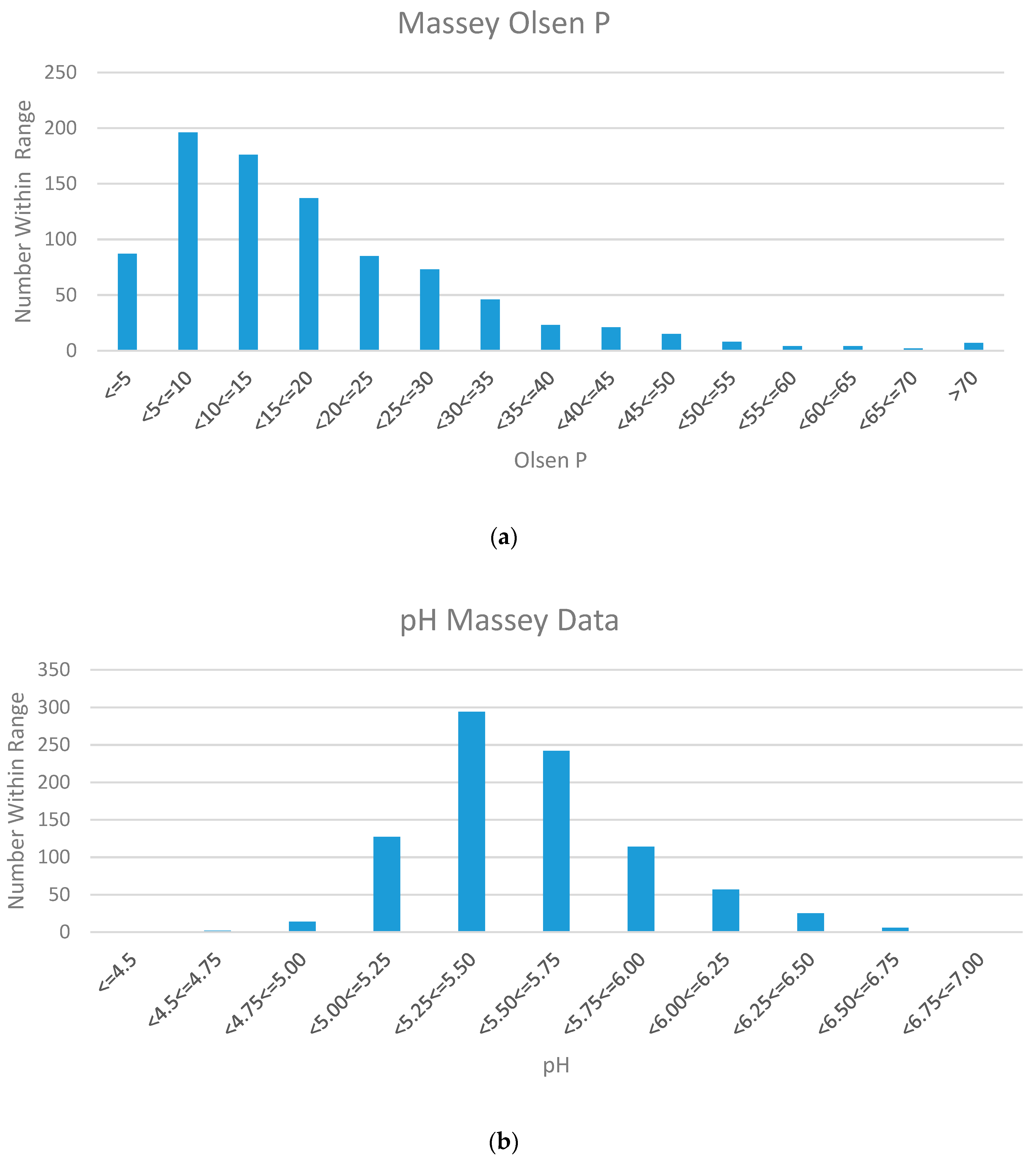
| Massey Olsen P | 18.1 | 13.9 |
| Massey pH | 5.55 | 0.33 |
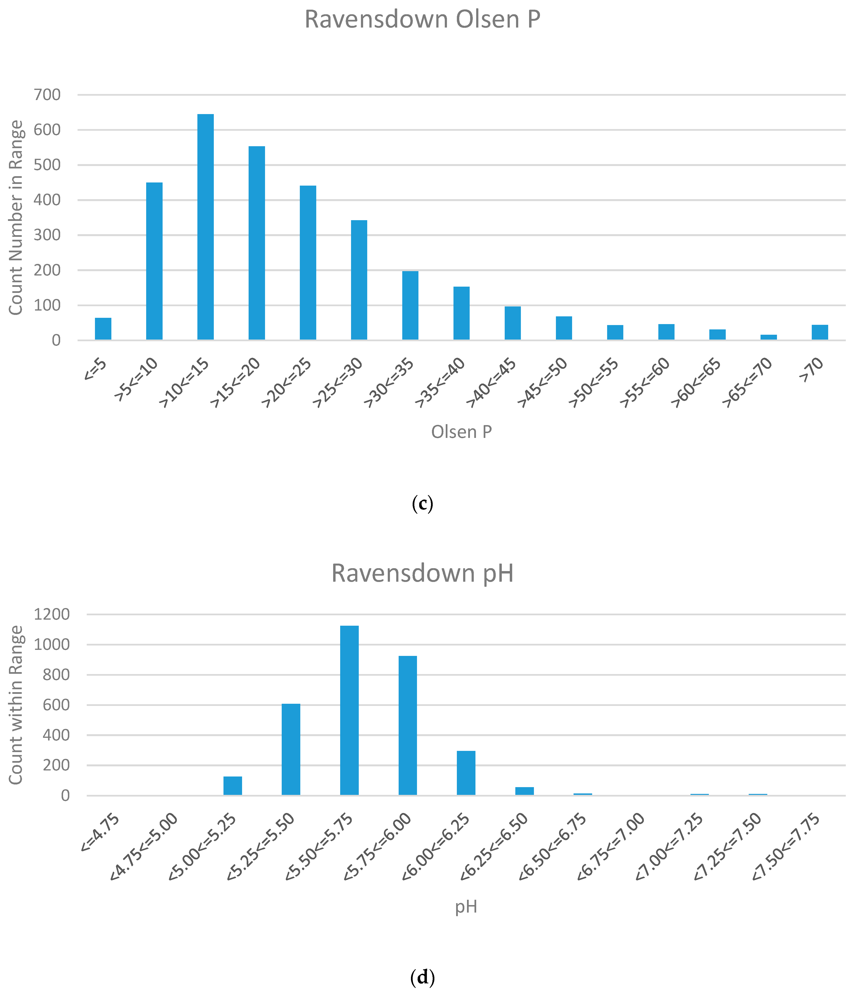
| Ravensdown Olsen P | 23.1 | 15.4 |
| Ravensdown pH | 5.72 | 0.32 |
| Data Set | Adj. R2 | Std. Err | F | p Value |
|---|---|---|---|---|
| Ravensdown Olsen P 1 | 0.47 | 11.21 | 2.319 | <2.2 × 10⁻¹⁶ |
| Ravensdown pH 1 | 0.71 | 0.17 | 4.688 | <2.2 × 10⁻¹⁶ |
| Massey pH 2 | 0.42 | 0.25 | 7.3 | <2.2 × 10⁻¹⁶ |
| Massey pH 3 | 0.42 | 0.25 | 7.3 | <0.0001 |
| Massey Olsen P 3 | 0.56 | 9.03 | 11.99 | <0.0001 |
| Ravensdown pH 4 | 0.42 | 0.24 | 24.53 | <0.0001 |
| Ravensdown Olsen P 4 | 0.27 | 13.21 | 12.53 | <0.0001 |
| Ravensdown Log OP 4 | 0.34 | 9.03 | 17.42 | <0.0001 |
| Massey Log Olsen P 4 | 0.46 | 0.25 | 8.5 | <0.0001 |
© 2019 by the authors. Licensee MDPI, Basel, Switzerland. This article is an open access article distributed under the terms and conditions of the Creative Commons Attribution (CC BY) license (http://creativecommons.org/licenses/by/4.0/).
Share and Cite
Grafton, M.; Kaul, T.; Palmer, A.; Bishop, P.; White, M. Technical Note: Regression Analysis of Proximal Hyperspectral Data to Predict Soil pH and Olsen P. Agriculture 2019, 9, 55. https://0-doi-org.brum.beds.ac.uk/10.3390/agriculture9030055
Grafton M, Kaul T, Palmer A, Bishop P, White M. Technical Note: Regression Analysis of Proximal Hyperspectral Data to Predict Soil pH and Olsen P. Agriculture. 2019; 9(3):55. https://0-doi-org.brum.beds.ac.uk/10.3390/agriculture9030055
Chicago/Turabian StyleGrafton, Miles, Therese Kaul, Alan Palmer, Peter Bishop, and Michael White. 2019. "Technical Note: Regression Analysis of Proximal Hyperspectral Data to Predict Soil pH and Olsen P" Agriculture 9, no. 3: 55. https://0-doi-org.brum.beds.ac.uk/10.3390/agriculture9030055