1. Introduction
The future of farming is not a trivial question to be answered [
1] since it is at the core of the future of humanity, with a population of about nine (9) billion expected by 2050 [
2], and it is closely related to various aspects of human life, e.g., poverty, political issues, etc. [
3,
4]. The need for increased productivity and sustainability is widely recognized, and so, various approaches have been proposed to address it, Climate-Smart Agriculture (CSA) being one of them [
5]. CSA is based on three “pillars” [
5,
6]: (i) maintain sustainability and resilience; (ii) increase productivity while adapting to climate changes; and (iii) reduce (or eliminate) gas emissions through mitigation.
To accomplish the goals set by CSA, recent technological developments in the area of Information Communication Technologies (ICT) can be exploited [
7,
8]. One of the aims of “green ICT” [
9] focuses not only on pushing for environmentally friendly ICT technologies, but also on enabling the use of ICT for the benefit of the environment [
10]. In this paper, the focus is on smart agriculture in the sense that ICT advances, and in particular those related to wireless communications [
11], are used to accomplish the goals of CSA, concerning olive groves. More specifically, the abundance of small and yet powerful devices that can be used as “sensors” (e.g., [
12,
13,
14,
15,
16]) in a Wireless Sensor Network (WSN) [
17], as “things” (e.g., [
18,
19]) in the Internet of Things (IoT) paradigm, or as “fog devices” in a cloud/fog computing environment (e.g., to support machine learning algorithms [
20]) for facilitating agricultural activities, was the motivation of this work. The case study that was considered refers to olive groves that are of high interest in the Mediterranean world, wherein most of the cases, farmers nourish a small number of acres scattered in a certain area. This intensifies the need for considering and seamlessly adopting the aforementioned technological developments, which will enhance the production line and ensure maximum quality of the product. Note that olive groves are a sensitive cultivation that requires special care [
21], since they are affected by various aspects, some of them being global warming [
22], the density of the plants [
23], etc. However the most important environmental agents that have been identified to impact their welfare are relative temperature and relative humidity.
As such, the research community is now focusing on various aspects and opportunities offered by smart farming and precision agriculture [
11], like sensor technologies (e.g., how humidity reacts with the sensor devices themselves [
24,
25,
26]), the advances regarding Unmanned Aerial Vehicles (UAVs) (e.g., how a UAV [
27] can co-operate with a WSN on the ground [
28,
29]), the exploitation of underground technologies [
30], the deployment of sensors for monitoring (e.g., [
31,
32]), the performance analysis of WSNs (e.g., [
33]), etc. Lately, however, there is a turn towards the exploitation of IoT and the advances it offers in regards to smart agricultural, e.g., [
34], through the use of cutting-edge, innovative, and low-cost wireless technologies, like ZigBee [
35], to establish reliable wireless communications [
36,
37]. It is noteworthy that these applications can be extended to support various domains related to agriculture, like food safety [
38] and security/privacy issues [
39]. Robotic appliances for agriculture have also been envisaged and partially developed [
40]. The previously mentioned technologies are expected to be further enhanced by the forthcoming Fifth-Generation (5G) of mobile communications, which will support massive numbers of various machines in small areas with a high bit rate and negligible latency [
41].
Still, for both the existing and (given the standardization process of 5G) the upcoming applications, one of the major challenges remains the support of multiple devices with a high bit rate, whilst processing the accumulated information almost instantaneously [
42]. Although this is not crucial for today’s agricultural applications, which are mainly targeted at environmental monitoring, nonetheless, it is considered a necessity for future farming where the need for real-time decision-making regarding the health of the farms, with low energy consumption and high automation, will drive the IoT’s functionality. For example, assume a harvesting machine for a special field of lemon trees that uses sensors to select lemons of a specific size and color. In this practical scenario, a large amount of data will be generated by the multiple sensors for every single fruit, which would need to be processed almost instantaneously with the aim of receiving real-time solutions (perhaps using sophisticated modern methods, like machine learning, e.g., [
43,
44]) regarding their quality.
To counter these issues, a popular approach incorporates the cloud/fog computing paradigm [
45,
46,
47], which offers computing, networking, and storage capabilities in close proximity to the end user, increasing data handling efficiency and minimizing response time [
48]. Consequently, the main contribution of this paper refers to the proposal of a cloud/fog computing architecture that is suitable for agriculture, i.e., in supporting smart time-sensitive agricultural applications, and to provide details around a low-cost prototype that is developed for the case of olive groves. Olive trees, as already stated, require a special type of cultivation for the final product (basically, olive oil) to be of high quality. The current “quality of service” agricultural procedures rely mostly on the experience of the individual farmers, accumulated over hundreds of years, while living in the Mediterranean, and in some areas going back to ancient times. However, the majority of the farmers cultivate a small number of acres, and in the majority of the cases, these are scattered in different geographic areas with possibly different characteristics (altitude, humidity, soil moisture, etc.). Although these environmental parameters may not differ significantly from grove to grove, nevertheless, even small changes in their value range may potentially lead to pest infestation and/or disease spreading, since most of the olive tree pathogens heavily count on these conditions to propagate. Additionally, wildfire outbreaks are a continuous threat to the Mediterranean lands, and in most cases, they are the derivative of relative temperature and humidity levels prevalent in the area.
To compensate for these olive grove hazards, an accurate and real-time monitoring mechanism of the environmental agents that lead to their appearance must be considered. Consequently, the central goal here is to present a cloud/fog network architecture that is affordable for small farmers that would like to take advantage of recent technological developments in ICT with the aim of sufficiently handling large volumes of raw data promptly. Contrary to previous implementations, the proposed approach allows for efficient correlation of the sensed measurements generated from different olive grove sources, and it is easily adjustable to latency constraints and load balancing requirements, meeting the necessity for heavy and almost real-time analysis of the acquired information. The farmers can then evaluate the information and take appropriate actions to counter potential threats before they manifest and become a serious problem. It is worth mentioning that, even though the presented case study revolves around olive groves, the considered cloud/fog computing architecture can be utilized for a wide range of agricultural applications, such as wildfire early detection, spraying scheduling, watering automation across multiple crops, etc.
The proposed architecture follows the main lines of the cloud/fog computing paradigm as it has currently evolved [
45], and it is close to the general framework presented by Guardo et al. [
47] for agriculture. In particular, the authors in [
47] revealed how such an architecture can be effectively used in time-sensitive agricultural appliances, and they evaluated it using latency as the crucial factor for determining early environmental conditions that occur at the deployment site. As such, the main focus here is on the presentation of the latency-adjustable cloud/fog architecture that successfully addresses the aforementioned challenges by dynamically mapping the system behavior to mirror the needs of the olive groves. To highlight its capacity and limitation, a demo prototype is deployed in the facilities of the Ionian University in Corfu, comprised of 28 sensory nodes, forming six (6) distinct WSNs, each equipped with their own sink node (i.e., six additional nodes, making a total of 34 deployed nodes). The WSNs are in turn connected to three (3) fog devices (forming a fog computing network), which are subsequently connected to the installed remote cloud server.
The evaluation process focuses on response time, processing ability, and load balancing. Experimental results show, following the principles of [
47], that such an architecture can indeed improve the farm of the future [
1] and, thus, deemed suitable for timely olive grove monitoring, by reducing the average response time of the system across all used platforms, when the need arises. Moreover, the research findings report on the efficiency of the approach and verify the expected system behavior, achieving significant throughput and overall highly balanced traffic load. In fact, through the augmentation of the cloud with extra fog functionality, it is proven that it is feasible to reach minimum latency and outperform conventional cloud-only approaches.
The remainder of the paper is organized as follows. In
Section 2, existing literature around the smart agricultural domain is summarized. The proposed cloud/fog computing architecture is described in
Section 3, and the corresponding system’s details are listed in
Section 4.
Section 5 portrays the role of the architecture in the context of olive grove monitoring, whereas
Section 6 deals with the experimental system’s setup and configuration properties. The evaluation process and its results are presented in
Section 7. Finally, the conclusions are drawn in
Section 8, which also reports directions for future work in the field.
2. Emerging Technologies for Smart Agriculture
The adoption of IoT, realized through WSNs, and the seamless migration towards a multidisciplinary model, e.g., [
49], have paved the way toward an increasing volume of novel research activities. As such, there exists a plethora of works, for example [
50,
51,
52,
53,
54,
55,
56,
57], that have investigated WSNs’ potential in the farming industry and the agricultural domain in general [
11]. Until recently, these domains faced many challenges, mainly due to the lack of wide-area connectivity, limited energy resources, and sometimes harsh environmental conditions that made the deployment of WSNs difficult or even impossible. Innovative and cutting-edge technological advances, however, have expanded the horizons with new low-cost enablers and energy-efficient wireless technologies [
30] (like SigFox [
58,
59], LoRa [
60,
61,
62], NB-IoT [
61,
63], GSM-IoT [
64,
65], and ZigBee [
66,
67,
68]), that take us to places previously unexplored, allowing us to test, administrate and record the dynamics of such systems in secure and credible ways [
69]. Some indicative works, that took place recently and have relevance to the current work, are listed below.
Many systems have been developed that focus not only on classical agricultural applications [
34], like crop monitoring [
53], disease countermeasures [
70], and pest detection [
71], but also on various other aspects of farming, as stated in [
1], where the needs of future agriculture were determined. These include (but are not limited to) management of underground planting [
72], modern drone spraying and control techniques [
29,
73], robotic enhancements [
74,
75], security and privacy matters regarding the sensed data [
39,
76], and of course, food safety and quality issues [
2,
38,
50]. A characteristic example of such approaches was followed in [
77], which reported on a control system that continuously analyzed the input from camera and sensor nodes deployed in crops and actuated the control devices according to given threshold values regarding various environmental factors. Another, found in [
78], presented an IoT system, called “MOCCA” (Cacao Monitoring System), that monitored climatic and soil factors, which influenced the growth of cacao trees to provide plans for protection against pests and diseases.
One of the main issues regarding the use of WSNs, however, is the energy required to keep the network “alive”. Many works have been reported in the literature that attempt to tackle this obstacle. An example is the work found in [
79], where a robust and green WSN node for fog platforms, called “FROG”, was presented for efficient power management in smart farming environments. In the current project, the WSN power consumption limitation is counterbalanced with the use of low-energy consumption sensory nodes (i.e., Arduino Uno devices), that have been proven to be power-efficient (e.g., in [
55]), along with attached power banks and load distribution mechanics, which push the energy boundaries, allowing for increased reliability. Alternatively, another important research topic refers to the careful selection and implementation of the base station, i.e., the node responsible for ultimately collecting the sensed data, usually for reasons of higher energy conservation and network lifetime prolongation, e.g., [
80]. In the current work, this challenge is tackled via the adoption of a higher-computational capacity Arduino device (i.e., the Arduino Mega), which played the role of the sink node, seamlessly interacting with the rest of the WSN sensory nodes.
Taking it a step further, the work in [
81] focused on the development of a WSN using a Raspberry Pi as a base station. According to [
82], there exists a plethora of research works in the literature that explore the potentiality of these devices in innovation and prototyping. In the case of [
81], the Raspberry Pi acted as a database and web server for collecting and managing agricultural data, whereas, for communication purposes, the ZigBee standard was adopted. A similar approach was followed in [
83] for sensor data acquisition and analysis. However, in both of these studies, no fog functionality was incorporated to assist the computational process, and in the first case, no hardware-oriented information was provided regarding the WSN nodes. On the contrary, in the present work, the Raspberry Pi is enhanced, not only with fog functionality, but also with the role of driving the data processing procedure, highlighting the potential to deal with time-sensitive environmental monitoring. In [
84], the authors proposed a scalable network architecture for managing farms in rural areas that embedded fog computing capabilities to increase coverage and throughput. Emphasis was given to a cross-layer based channel access and routing approach that could combine the input from multiple networks. However, their work did not involve the use of low-cost open access hardware and software solutions offered by Arduino and ZigBee, respectively, as in the current work. ZigBee has been around for quite some time now (e.g., [
85]), and in combination with WSNs, it has proven a reliable and affordable protocol for realizing smart agriculture (e.g., [
86]), thus making it the preferred communication protocol here.
On a different path, the authors in [
87] dealt with the deployment of a WSN consisting entirely of Raspberry Pi nodes for implementing a smart agricultural model. In their system, the monitoring of the WSN was accomplished by a Graphical User Interface (GUI) application, programmed using “MATLAB” software, installed on the base station’s board. Diving deeper into developed prototypes, which also find relevance for the current work, the authors of [
88] presented a WSN testbed to monitor the micro-climate of grapevines in Sicily, with the aim to manage spring period hazards. The WSN was then compared to a traditional fixed meteorological station and was shown to be more efficient in monitoring the local environmental conditions. On the other hand, the researchers in [
89], similarly to the current work, focused specifically on olive groves. Olive trees, like grapevines, are very susceptible to diseases and weather changes, thus requiring continuous care to produce high-quality products (mainly olive oil). Therefore, the authors described the design and deployment of a WSN based environmental monitoring system, named “MasliNET”, that utilized low-power sensors to keep watch over the olive groves’ micro-climate in an energy-optimized way.
Under the scope of the emerging hybrid cloud/fog paradigm, the authors of [
47] proposed a framework for precision agriculture comprised of two distinct fog layers adopting different computational capabilities. As shown through simulation results, one of the most important benefits of employing a fog computing functionality to support the cloud is the load-balancing properties of the hybrid solution. Correspondingly, in [
90], the authors followed a similar approach to the one presented in the current work, with the aim to demonstrate the advantages offered by flexible IoT devices, such as Arduino sensors and Raspberry Pis, in supporting agile development for agricultural applications. In this context, they described the design and implementation of a system prototype, deployed in North Wales, and its requirements regarding its operational effectiveness in managing hydrological, soil, water, and land environments under harsh conditions. However, in their approach, the Raspberry Pis acted as an Internet gateway with no further functionality, whilst in the current work the Raspberry Pis inherit fog functionality to further extend the computational capabilities of the cloud infrastructure. Additionally, the work found in [
91] presented a service processing mechanism that was seamlessly embedded in a cloud/fog environment, with the purpose to augment the networking and automation aspects of the cloud platform and improve the computing speed of the underlying IoT (which encompassed Raspberry Pi sensory devices). Experimentation results showcased the potential at reducing network transmission costs and enhancing the real-time environmental monitoring, while at the same time providing user-friendly ways to store and present the accumulated data. Finally, the work in [
92] presented a cloud-oriented irrigation controller and the development of a multimedia platform for precision agriculture, named “PLATEM PA”, that used aerial imagery from crops and periodic soil/atmospheric sampling processes to visualize the ongoing situation in the fields and potentially block the crop spraying procedure.
As already mentioned, the term “smart” in this work corresponds to the use of modern ICT for the benefits of agriculture and the protection of the ecosystem. Note that IoT and WSNs are not always clearly separated, and it is expected that in the future, both will be included under the Fifth-Generation mobile phone systems’ (5G) umbrella. The increasing number of IoT and WSN installations will require high data rates of many Gbps; ergo, the introduction of 5G will allow the wireless networks to meet the particular requirements [
41]. Additionally, 5G will enable the interconnection of many WSN and IoT devices; thus, access to information and data sharing will be available anytime to anyone. Moreover, human-centric communications are expanding to include machine-centric communications, offering more flexibility than previous generations [
42]. Under this light, 5G is an enabling technology that will allow for new opportunities in applications related to IoT and WSNs. These opportunities—apart from the higher bandwidth, minimal time delay, and massive device support—will include “intelligent” decisions for numerous scientific areas, agriculture being one of them [
93]. As mentioned in [
93], in the future, agriculture will require the fast processing of large amounts of data to control UAVs, ground vehicles, sensor nodes, harvesting machines of various types, etc., and 5G is expected to provide for these increased demands and seamlessly manage them. As such, the proposed three-layered architecture fits perfectly in this context since it is simple to implement and at the same time capable of sufficiently handling, in a timely manner, large volumes of raw data generated at the olive groves. In addition, its functionality is easily adjustable to network changes (or even adaptable to other agriculture habitats, e.g., grapevine crops), mapping its activity to the farmers needs and modifying the sensing behavior to mirror the necessity for faster field measurement analysis. To the best of the authors’ knowledge, this is the first implementation that is capable of a self-acting operational conformation based on the local decision-making process at the fog layer.
3. The Proposed Cloud/Fog Computing Architecture
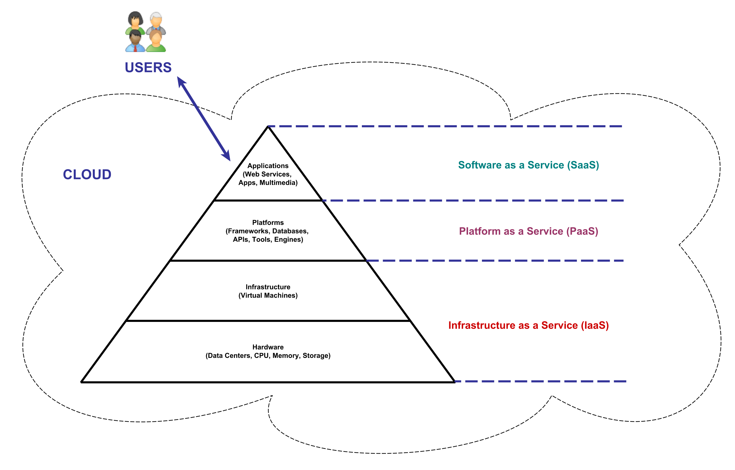
Starting from the cloud computing paradigm, the offered services follow an upward categorization scheme, which can be contextualized with layers forming a stack, as depicted in
Figure 1. The basis of the stack is comprised of the hardware layer that is realized inside data centers [
94], i.e., large infrastructures typically containing thousands of servers [
95]. Therefore, the lowest layer consists of the hardware that is part of the data center infrastructure (basically comprised of storage, network connectivity, and computational power). However, offering “hardware as a service” is not an easy task; hence, the first layer usually corresponds to the “Infrastructure as a Service” (IaaS) layer, where resources, e.g., Virtual Machines (VMs), formed by various levels of computational power, memory, and storage, along with the data centers’ hardware, are offered to the end user [
96].
Moving up the stack of
Figure 1, the “Platform as a Service” (PaaS) layer abstracts the necessity to deploy applications on VMs, by introducing the necessary platforms that will facilitate the applications, whereas the “Software as a Service” (SaaS) layer offers the applications themselves, e.g., web-based services, multimedia, business apps, etc., to the end user. The particular architecture proposed next takes into account this simple layering model focusing on the IaaS layer, which is considered to be the most suitable for the corresponding agricultural applications. Still, notice that the proposed architecture can be utilized for PaaS and SaaS as well.
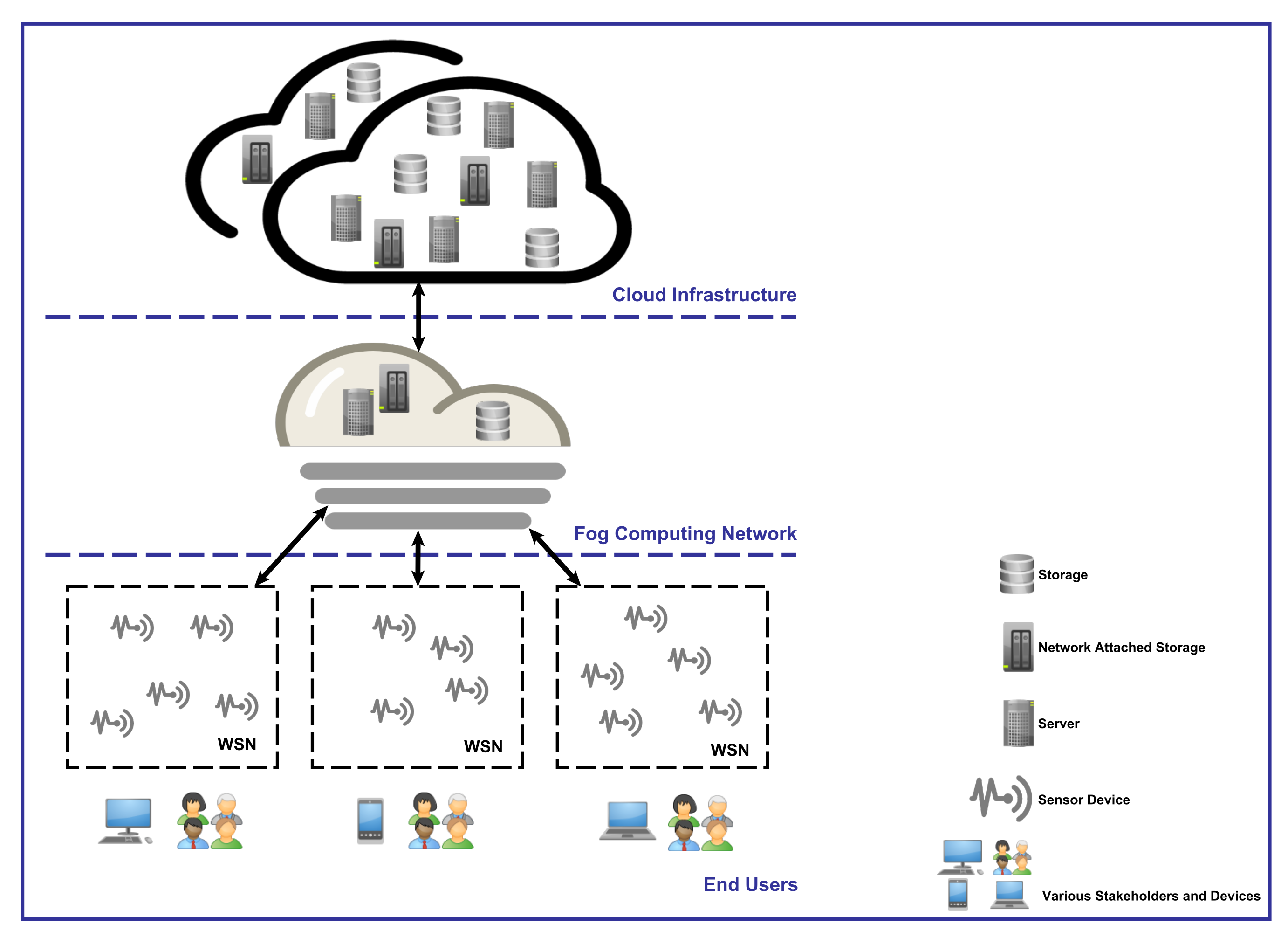
It is a common case for cloud services to employ multiple data centers taking into account various parameters like proximity to the users and energy consumption [
97], thus forming a cloud computing network, as depicted in
Figure 2. The capabilities of the data centers, illustrated in this figure as storage (conventional and network) and server (computational power and support for platforms/services), are assigned dynamically to the users based on their demands. As already mentioned, data centers are expensive and generally not close to the end users. To address these issues and provide a lower cost solution, the fog computing paradigm was adopted. Fog devices, that are less expensive and smaller than the data centers, offer similar (even though with less computational capabilities) services, in close proximity to the end users [
98], forming a fog computing network, as also shown in
Figure 2.
The end users, on the other hand, correspond to the various agricultural applications, which have already been mentioned, in addition to the farmer, which is responsible at the end of the day for receiving the processed data, through the cloud/fog computing network infrastructure, and who then has to interpret them and take appropriate actions. Therefore, the end user is not just the farmer and his/her personal devices (smartphone, laptop, personal computer, etc.) that he/she uses to gain access to the data, but also the various devices that generate the data. The latter are illustrated in
Figure 2 as sensor devices.
It is clear from the outlined three-layered cloud/fog computing network architecture, depicted in
Figure 2, that an end user device can sometimes be close to the cloud infrastructure, but in the general case, it will be closer to the deployed fog devices. As a result, the presented system architecture takes action with lesser delay and saves bandwidth in the network, reducing network congestion near the cloud servers and avoiding the creation of traffic bottlenecks. Consequently, the purpose here is to move functionality from the cloud to the fog, in a way that will prove useful for serving agricultural applications, whilst maintaining the overall system cost as low and accessible to the olive growers. Besides, these are considered main goals of future smart farming, and so, throughout this work, there are references to how the presented architecture and system address these aspects.
4. System Overview
Having presented the proposed cloud/fog computing network architecture in the previous section, it is now feasible to move on and provide a layer-by-layer detailed description of the system itself and its separate components. Hence, each node making up the cloud/fog network system across the networking path, from the WSN nodes (i.e., the deployed sensors for monitoring the olive groves in the current case study), to the intermediate fog devices, to the centralized cloud infrastructure, alongside various other implementation and networking issues are described in detail.
It is worth mentioning that the proposed cloud/fog system uses open-source hardware and software platforms (i.e., Arduino, Raspbian, ZigBee, etc.) and is low-cost, low-power consuming, and highly scalable, depending on the number of deployed sensors in the olive groves. This makes it an excellent, easily adaptable, and viable solution for farmers looking to invest in such an intervention.
The lowest level of the architectural hierarchy is implemented for the area of interest (i.e., the olive groves) using sensory nodes, which in turn synthesize a WSN governed by a selected central node, i.e., the sink node. Because of their integrated capabilities and the ability to add more nodes along the way, increasing the coverage range and overall scalability, WSNs are considered an excellent candidate for agricultural and farming applications [
54].
The sensor nodes in the current project were constructed by Arduino micro-controller boards. Arduino [
99] is an open-source electronics platform, popular for its usability and interoperability, which can easily embed a variety of components and modules to extend the functionality of the involved nodes. In particular, the nodes comprising the WSNs for each olive grove include an Arduino Uno Rev. 3 (or just Arduino Uno), which is built on top of the Atmel ATmega328P microcontroller, with a clock speed of 16 MHz and 2 KB of SRAM.
Table 1 summarizes in detail the Arduino Uno’s technical specifications [
100].
On the other hand, to prolong the WSNs’ lifetime and provide outdoor power support to the nodes, Sandberg Solar Powerbanks were utilized. The specific model was designed to be maximally resilient and even rainproof, featuring two USB ports, with a maximum capacity of 16,000 mAh and built-in solar panels to enable energy harvesting from the sunlight.
Taking it a step further, to enable wireless communication, the sensor nodes were enhanced by an Arduino Wireless SD Shield and with a Digi XBee-PRO S2C module attached on top, which utilized a wire antenna for actuating wireless communication without the requirement of additional adapters, while at the same time permitting the exchanged data to be saved on micro Secure Digital (SD) cards. The Digi XBee-PRO S2C module operated at 2.4–2.5 GHz with a maximum transmission rate of 250 Kbps, encapsulating three different protocol stacks, the first two being the 802.15.4 and DigiMesh and the last being the ZigBee protocol [
35], which specified a suite of high-level communication standards, incorporating an IEEE 802.15.4 defined Carrier-Sense Multiple Access with Collision Avoidance (CSMA/CA) protocol used to create wireless networks built from small, low-power digital radios [
81]. Moreover, the XBee module offered increased security through data packet encryption [
101], a subject of the utmost importance when it comes to data integrity, in order to facilitate secured transmissions and, in the end, acquire reliable information, without the constant threat of measurement tampering from exogenous factors, such as human intervention.
While the Arduino Uno is the most widespread and well-known Arduino board since it is heavily tailored towards new-comers in the world of electronics, the Arduino Mega 2560 (or just Arduino Mega) features a relatively higher amount of SRAM, specifically 8 KB, and boasts a larger number of pins and a faster microcontroller, capable of supporting the needs for memory usage and processing power by the agricultural applications at hand. For this reason, it was considered a suitable solution for hosting sink node properties in the constructed WSNs and responsible for collecting and managing all of the sensory data of its respective WSN. The complete set of technical specifications of the particular Arduino Mega [
102] is presented in
Table 2.
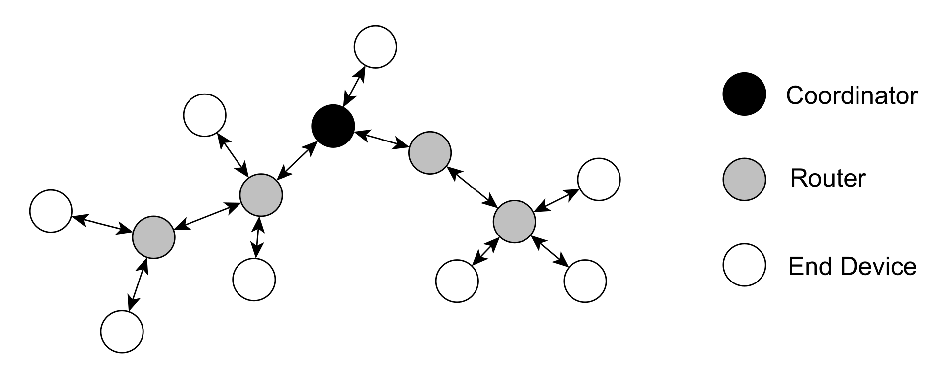
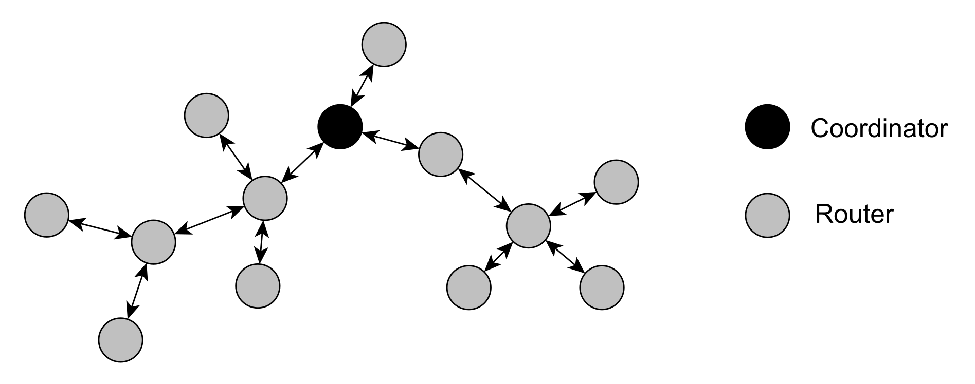
The combination of Arduino Uno and Mega nodes led to the formation of fast, flexible, and accessible WSNs, which could also be further augmented if the need arises, by simply installing more nodes or by attaching more modules on their boards. The most important aspect, nevertheless, remains their inherent ability to connect seamlessly and mold scalable networks. Diving deeper into the connection scheme, since all nodes used the ZigBee protocol for communication, according to [
103], three basic types of roles were present in the system. The coordinator was a key structural component, tasked with setting up the network and initiating other critical procedures regarding its functionality, such as security and self-healing mechanisms. Additionally, the coordinator had the task of choosing an appropriate Personal Area Network (PAN) id, which was an identifier shared among all nodes of the same WSN, along with a free channel for the latter to operate on, ultimately establishing a routing plan. As showcased in
Figure 3, there only one coordinator in a given WSN could exist; hence, in the current system, this role was assigned to the Arduino Mega.
In comparison, the routers were the most generic device types, and so this, was the case for most of the deployed nodes. These nodes acted as intermediates to convey data from devices that were too far away (in network distance) to interact directly with the coordinator and exchange data, i.e., the end devices. Contrary to the previously mentioned types, the end devices were permitted to “sleep” occasionally to conserve their energy. However, they were restricted to communicating with a single node, referred to as their “parent”. End device parents were in this way responsible for buffering messages until their associated end devices “woke up” to receive them. The router and end device nodes in the described system were the Arduino Uno sensors.
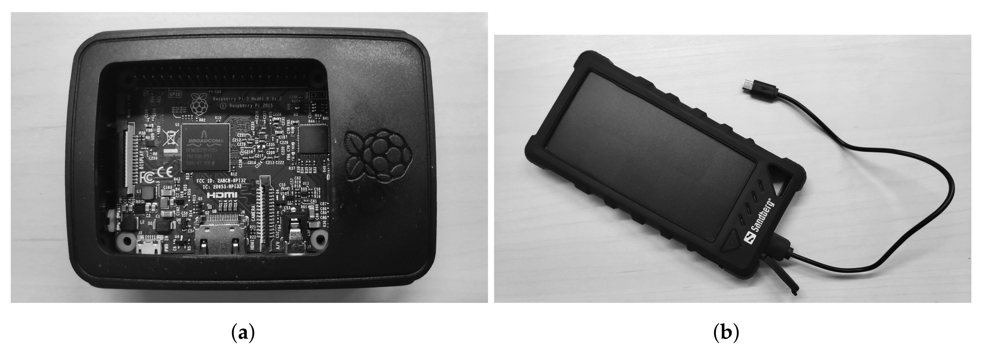
The middle layer of the proposed architecture, i.e., the fog computing network, included Raspberry Pi [
104] devices, each one responsible for collecting and computing data from one or more WSNs through serial connection with the corresponding Arduino Mega. More specifically, the fog devices were the Raspberry Pis 3 Model B, the earliest model of the third-generation of the Raspberry Pi series [
18]. This model was selected due to its low-cost and low-power consumption attributes and its availability for wireless (using a Wi-Fi adapter) and Bluetooth connectivity. Its board operated with a Quad-Core 64 bit processor, running at 1.2 GHz [
87], and came packed with 1 GB of RAM. Essentially, it was a small computer board that supported several different operating systems. For the current work, the Raspberry Pis used as fog devices were powered by a Debian-based Linux operating system, named Raspbian, which was also the recommendation of the Raspberry Pi Foundation [
81], and could be booted by an external SD or micro-SD card.
Table 3 highlights the most notable technical specifications of the Raspberry Pi 3 Model B [
105]. For energy conservation, the used Raspberry Pis were also enriched with a solid protective outer-shell along with solar power banks. Both devices are illustrated in
Figure 4.
It is understandable that unlike the Arduino nodes, the Raspberry Pis had increased computational and processing power, with the dynamic quality of turning them into personal computers [
106], sensors [
87], network tools or gateways [
90], database managers [
81], web servers [
83], fog devices [
47], etc. Consequently, they were considered an ideal solution for locally processing data from olive groves and, if necessary, subsequently relaying this information to a centralized cloud computing infrastructure through local area network connectivity, such as Third-Generation (3G) mobile telecommunications, for further computation. The latter formed the third and top layer of the network architecture, which is fully analyzed, for the case study of olive groves, in the sequel.
5. System Application for the Olive Groves
Based on the aforementioned, the overall network behavior could now be outlined with relation to olive groves. Additionally, application scenarios are provided to contextualize the appropriateness of the approach.
5.1. Deployment in the Field
The proposed system incorporated various technologies, making use of smart low-cost devices and the IoT paradigm, to enhance agriculture and help farmers make the best out of their olive groves with affordable interventions.
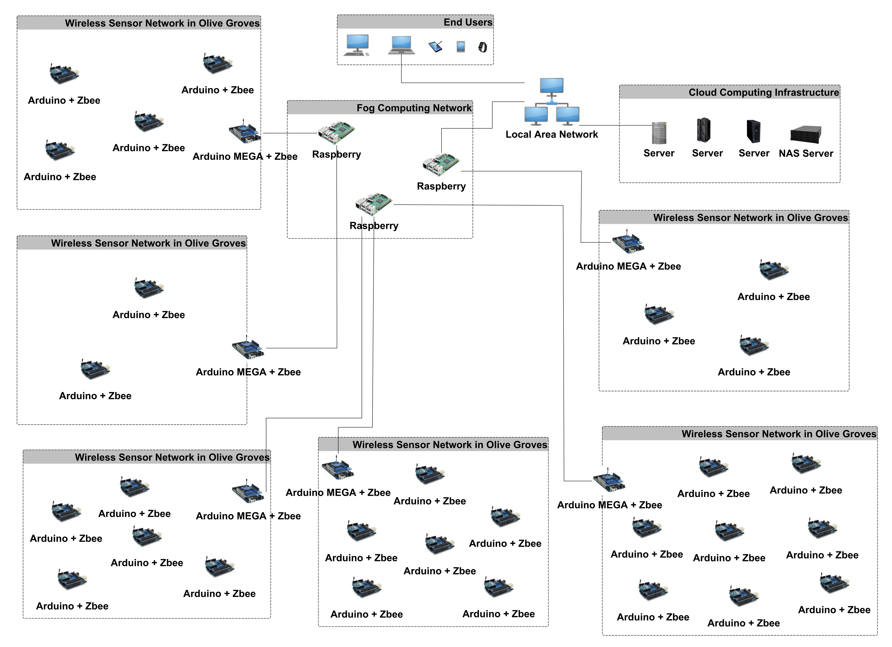
Figure 5 depicts the system’s network architecture when a post-deployment in the field of interest occurred to monitor six olive groves. Note that, even though the case study referred to olive groves, the proposed system may be easily modified to support many different agricultural habitats, like grapevine crops.
The first stage of deployment included setting up the various WSNs in each olive grove. Based on the number and size of the olive trees, a number of Arduino sensors were employed, hooked up with a Digi XBee-PRO S2C module for routing and communication purposes. Key to the accountability of any deployed WSN is the ability of its sensors to make accurate measurements of their surroundings, even under harsh conditions. Equally critical to the applications’ success is the selection of the appropriate environmental parameters to monitor. This is the reason why for the current work, all sensor nodes were made of an Arduino Uno with attached sensory modules for sensing environmental data regarding the humidity, soil moisture, temperature, and Ultraviolet (UV) ray intensity of their assigned area, at regular intervals. These variables were considered critical for olive groves in the Mediterranean basin, to surveil the health of the olive trees successfully and ensure the high quality of the final products, mainly olive oil.
Conversely, the sink node, as already stated, consisted of an Arduino Mega, responsible for collecting the sensed data from all the sensor nodes in the olive grove. The sensed data were transmitted wirelessly from one sensor node to the next and towards the sink node, on predefined paths set by the underlying ZigBee protocol dynamically during and after the initialization of the WSN. When the sink node was in range of another sensor node, then they could communicate directly and exchange data packets. On the other hand, if the sink node was out of range, then the data were transmitted to the nearest node acting as a ZigBee router and then forwarded accordingly to the next node on the routing path on a per-hop basis.
Moreover, each Arduino Mega device acted as a gateway for relaying the collected data to the nearest fog device, i.e., the Raspberry Pi overseeing the particular WSN, via an internal connection. Each fog device may connect with one or more Arduino Megas based on the geographical distribution of the olive groves, and therefore, may receive data from one or more WSNs. This, in turn, was attributed purely to the geolocation variance of the Arduino Mega devices and the Raspberry Pis, since in the examined case of olive groves, the monitored acres and, thus, the installed WSNs, may be scattered in different geographic areas with possibly different environmental properties (e.g., altitude, soil moisture, humidity, temperature, level of sunlight, etc.).
Moving on, the fog devices acted as intermediates to communicate the data to the remote cloud computing infrastructure through an external network channel. The latter contained powerful servers and data centers capable of performing computational demanding tasks regarding the collected data generated in all monitored olive groves. To support this procedure, minimize the network traffic and congestion, and optimize the response time, coverage and agricultural precision, the various fog devices could be upgraded to include cloud elastic resources, offloading the cloud’s computational power to the edges of the network and close to the end users [
107], i.e., the olive grove sensors and ultimately the farmers. To achieve this, upon reception of the data, depending on the implementation, the Raspberry Pis, instead of relaying the data deeper into the cloud, could act as mini cloud data centers, augmenting the system and performing on the spot the necessary data treatment in a more secure and effective manner, achieving lower latency and higher precision, based on local contextual information, such as regional environmental and network conditions, detailed geographical distribution of the Arduino sensors, WSN’s behavior awareness, etc., [
108].
In any case, after the data were successfully accumulated, analyzed, and processed, either by the cloud computing infrastructure or the fog computing network, an analysis report regarding the health of the olive groves and the soundness of the environment was procured. This report must reach the source, i.e., the WSN and their respective sensors, and ultimately the farmers, so they could monitor and look after their olive groves in an almost real-time manner. In this way, they would be able to take necessary countermeasures and precautions if the need arises (e.g., in case of fungi diseases), through specialized treatment targeted at the specific conditions existing in each olive grove according to the analysis generated by the corresponding sensed data. The same applied in cases of extreme environmental conditions (such as extensive rain seasons, summer fires, intense winds, etc.), which may require instantaneous decisions for the generated product (mainly the olive oil) to remain intact and of high quality, and so, the response time of the system must be kept at the minimum possible level. As already highlighted, this was one of the main goals of the current cloud/fog system architecture, and thus, a more in-depth discussion revolving around its dynamics is held in the following section, which presents the experimental prototype system. With that being said, it is crucial first to acknowledge existing olive tree hazards that motivated the adoption of the proposed system.
5.2. Importance of Time-Precision Monitoring in Olive Groves
Olive cultivation is the most widespread tillage in Greece (since olive oil is one of the main exportable products), which is why olive plant protection needs special attention. Besides, olive trees are sensitive to specific pathogens and pests; thus, precise monitoring of their health is required to facilitate targeted countermeasures and guarantee the quality of the product if the need arises. In order to analyze the health and acquire important information, close monitoring of the environmental parameters that lead to certain phytopathologies is necessary. These parameters may vary in nature; however, according to [
109], for the case of olive trees, these can be summarized to the degree levels of moisture and heat present in the ecosystem. Below, some characteristic cases are listed to showcase and justify the use of the specific sensors in the current system approach.
Olive trees generally require well-drained soil and a sunny position to avoid the potential spread of pathogens and fungi [
110,
111,
112]. One of the most severe olive tree diseases is olive peacock spot, which can cause significant loss of olives and affect the leaves and is attributed to the
Cycloconium oleagineum fungus [
113]. The fungus is easily spread by the weather and/or by insects, so it is near impossible to contain. Infections mostly take place during seasons of heavy rain or weather conditions of very high relative humidity or/and relatively low temperatures (6–12
C) [
114]. Another, widespread disease, with high occurrence in Greece, which attacks the olive fruit, is violet scale, which appears due to the presence of
Camarosporium dalmaticum fungus [
115]. The latter’s growth rate increases mainly during the prevalence of high temperatures of 20–30
C (optimum 30
C), while temperatures below 15
C are unfavorable for its development. Olive anthracnose (commonly known as Pastella to olive growers) is also a dangerous olive tree disease, caused by
Gloeosporium olivarum [
116]. In Greece, it mainly appears in the region of the Ionian Islands (including Corfu), during autumn, with high humidity/ Its characteristic symptom is rotting olive fruits. The ones that fall on the ground are found with a pink slimy mass on their surface, while those that remain on the tree quickly deteriorate. On the other hand, a very difficult olive disease to cure is shoot necrosis. The causal agent has been identified as the fungus
Phoma incompta [
117], and the symptoms of the disease are reddish-brown lesions on young shoots, withering of leaves, cankers on older shoots, and shoot/trunk necrosis. Infections occur at temperatures of 10–33
C in rainy seasons (ergo, they appear mainly in places where there is rainfall), whilst the phenomenon progresses faster during the summer months. As a result, considering that Corfu is characterized throughout the year by heavy rain activity and high heat during the summer, it becomes an excellent candidate for spreading this particular disease.
Besides the diseases, a major threat for olives groves remains pest infestation. There are numerous phytophagous parasites that infect olive trees, but three of the most prominent dangers are black scale, olive moth, and olive fruit fly. The first, with the scientific name
Saissetia oleae, excretes a significant amount of molasses, which is complex to eliminate, depreciating the value of the olives ready for greening. The parasite thrives in high temperatures and atmospheric dryness [
118]. The second is scientifically known as
Prays oleae and significantly alters the quality of the oil, hence producing great losses for the farmers, since it feeds on three different parts of the trees (these being the leaves, the flowers, and the fruits). The greatest ally for the pest is winter and low temperature [
119]. The last, scientifically named
Bactrocera oleae or
Dacus oleae, can wreak havoc on olive production under favorable conditions [
120]. The olive fruit fly is the number one threat to olive groves in Corfu, Greece, meeting its peak during rains and mild temperatures [
121,
122]. The damages from the fly are twofold, quantitative and qualitative. The former is because it results in a reduction in the yield of olives, while part of the production is lost due to the premature falling of the attacked fruit. The latter is due to the high deterioration in the quality of the oil caused by high acidity levels originating from the pest.
The aforementioned concerns are just a few of the most common diseases and pest infections. Of course, there exist many more; nevertheless, their mutual characteristics relate to the prevailing environmental parameters that help accelerate their appearance. However, these parameters can also play the deciding factors in their early detection and prevention. By identifying these crucial conditions in each natural habitat, it is feasible to deploy efficient countermeasures in a timely manner with targeted interventions, avoiding hazardous situations that will affect and potentially destroy olive production [
123]. These countermeasures include, but are not limited to, chemical treatments, bio-solutions, special olive medicine, autonomous spraying/watering mechanisms, specific pest traps, pruning processes, fruit ripening, etc. It becomes evident that having this information available in real time allows the farmers to launch efficient ways to counterattack and balance the effects caused by environmental factors, which help the olive fungi and parasites to flourish, without endangering the rest of the environment, the flora, or the olive trees themselves. Furthermore, the analysis of the data and the temporal correlation of sensed variables will allow for future decisions regarding the general health of the olive groves and provide feedback to agronomists regarding potential new treatments targeted at the specific conditions prevalent in different micro-climates.
At this point, it is worth mentioning that an additional danger to olive groves relates to one of Greece’s most hazardous states of emergency, i.e., wildfires. In fact, according to Greece’s Fire Brigade (GFB) official statistics, 8006 forest fires have been recorded during the year 2018 [
124], while initial predictions showed that for 2019, the number was much higher. On Corfu Island alone, based on the most recent official report of GFB, in the year 2018 alone, 174 wildfires were recorded, burning around 84 acres of land, a great percentage of which consisted of farming lands and olive groves [
124]. Obviously, to be able to handle a potential crisis and make appropriate adjustments to protect the lands, a deeper understanding of the hostile conditions leading to these events must be undertaken. However, the biggest weapon against fires is early detection, and to this end, precise monitoring of the environmental conditions, such as levels of drought, relative humidity, and spikes in temperature, will ensure the survival of the olive groves.
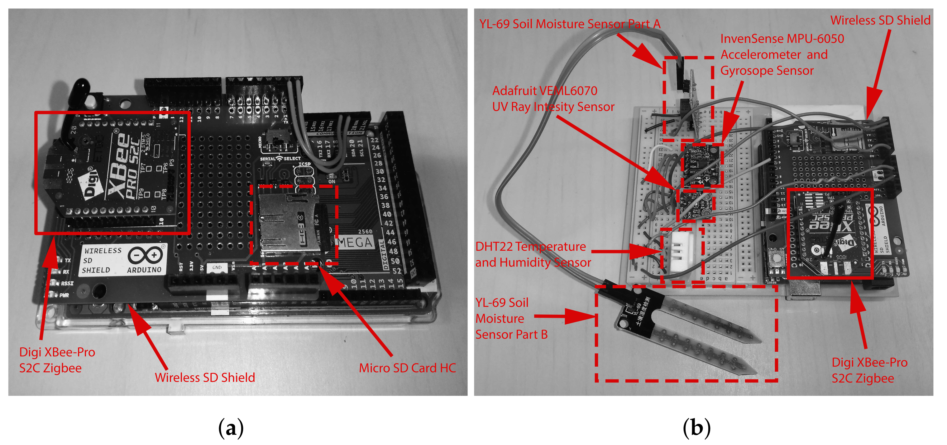
For the above reasons, and as already stated, four environmental parameters that heavily impact the olive groves were taken into consideration in the current project, i.e., temperature, humidity, UV ray intensity, and soil moisture, in order to equip the Arduino Uno devices with the appropriate sensory modules. As such, the first two of the set came packed together in the DHT22 (also known as the AM2302 reference) digital temperature/humidity sensor. The DHT22 sensor was able to measure temperatures ranging from −40 to +125
C with an accuracy of +/−0.5
C. It could also calculate relative humidity levels in the atmosphere from 0% to 100% with an accuracy of +/−2%. However, depending on the harshness of the environmental conditions in which the sensor was deployed, this value could vary (e.g., from +/−5% at extremes to even 10%). The sensor could perform a measurement every 500 ms, i.e., twice per second. The third sensor was an advanced UV light module called Adafruit VEML6070 UV with an I2C protocol interface, which possessed linear sensitivity to solar UV light and could be easily adjusted by an external resistor. The fourth sensor was a YL-69 soil hygrometer (or humidity and soil moisture detection sensor, in other words) and consisted of two components, the first being an electronic circuit with a built-in digital potentiometer, which was used to adjust the sensitivity, and the second being a probe with two pads, which was placed in the ground to detect the water content in the soil. Both of these sensor models were low-cost and easy to install and adjust. Lastly, each Arduino was equipped with an InvenSense MPU-6050 sensor, which was essentially an accelerometer/gyroscope sensor and was placed on top of the Arduino boards to notify the farmers in cases where the nodes were for some reason misplaced by weather conditions, accidentally moved by a passing animal, or stolen by other individuals.
Figure 6 depicts the two Arduino models used (i.e., the Mega and the Uno), with their attached components and sensors, after their assembly and before deployment.
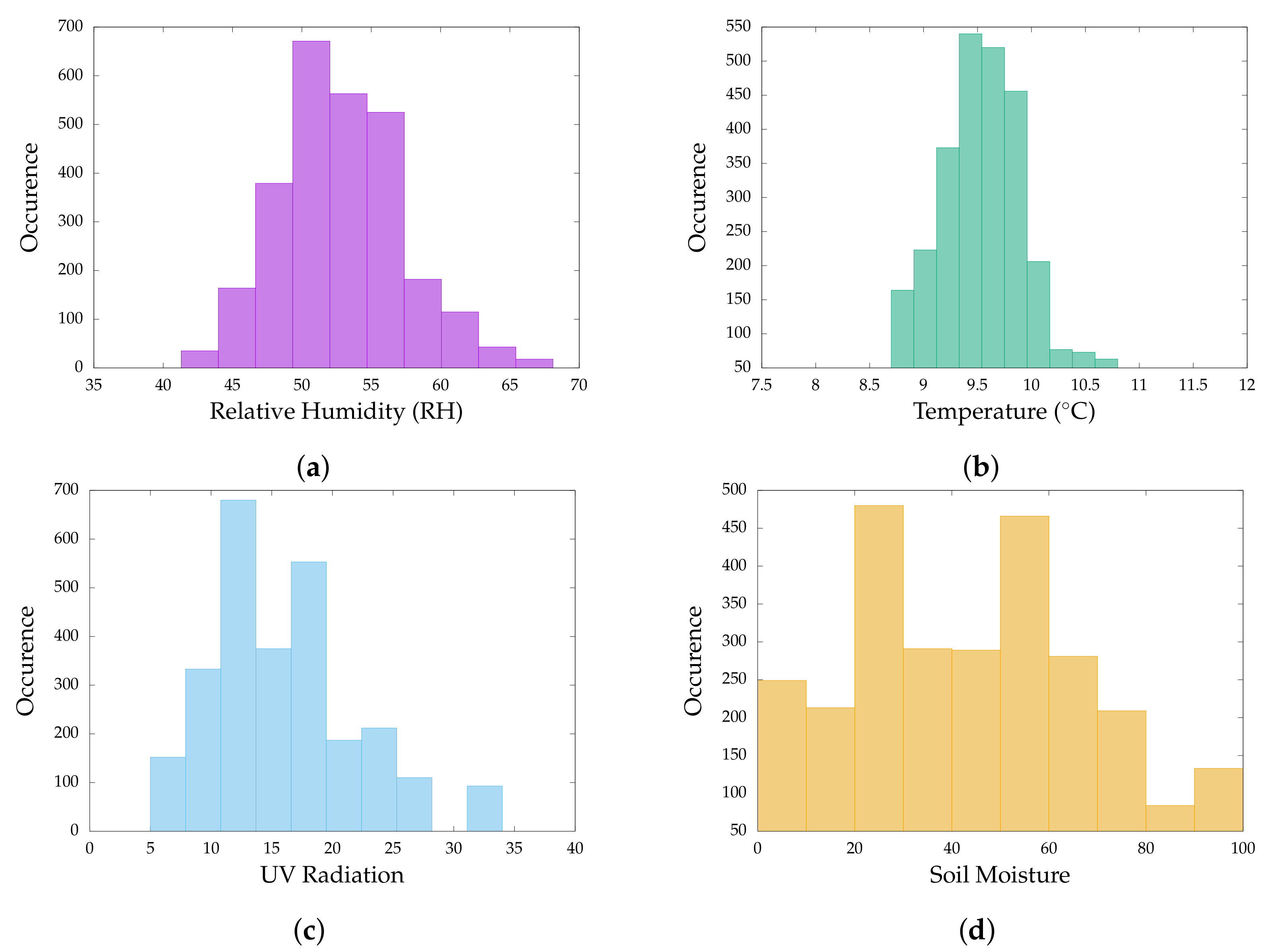
Actually, in order to procure a more accurate image of the sensory attributes regarding important agricultural aspects of olive groves, based on the unique weather conditions that were prevalent in each area and heavily affected the health of the trees, the sensors were deployed for a short period of time at a real olive grove in Corfu.
Figure 7 jointly presents the measurements’ dataset acquired during the experiment over a 20 min period. As was observed, the relative humidity values were all concentrated around 50%; the temperature was fairly stable at around 9.5
C; UV radiation was clustered around 15%; whereas soil moisture did not seem to follow any particular pattern. The last was attributed to the variance in the soil’s underground water levels at different olive tree root locations. The measurements were indicative of the achieved precision, a fact of utmost importance for successfully correlating the spread and speed evolution of pathogens, pest, or wildfires with the environmental factors that affect the olive groves at the micro-level of each olive tree. Note that the particular dataset was at its early stages of analysis, and thus, a full presentation of the retrieved results is beyond the scope of current work and part of ongoing research. However,
Figure 7 validates the effectiveness and precision of the sensing process.
6. Experimental Setup
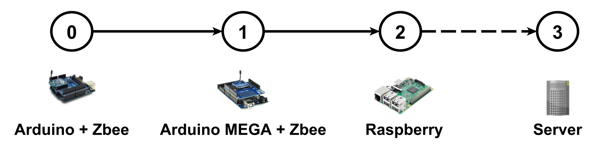
To further evaluate the proposed cloud/fog architecture and verify its effectiveness, in regards to smart agricultural applications and specifically small-scale olive-groves’ monitoring, an experimental prototype system was designed in a closed control laboratory environment in the facilities of the Ionian University, located on Corfu Island. The objective of the conducted experiments was to capture the behavior of the system in terms of latency before and after the deployment of fog functionality. In the first case, the WSNs would communicate with the cloud computing infrastructure, via the intervention of the Raspberry Pi gateways, whereas, in the second case they would exchange data with the intermediate Raspberry Pis, forming the fog network and responsible for some processing activity at the edges of the cloud. The information flow of the latter case is depicted in
Figure 8, where the dotted arrow line between the Raspberry Pi and the cloud server (i.e., between steps number two and three) reveals that the data arriving at the Raspberry Pi may undergo processing directly at the fog computing network or may be forwarded to the remote cloud server for further computation.
The experimental prototype was inventively designed to capture the architecture illustrated in
Figure 5. Ergo, it included six (6) WSNs, each with its own sink node (i.e., six Arduino Mega were used) and a different number of sensory nodes to force diversity in the resulting topologies, mirroring the needs for various sized olive groves.
Table 4 showcases the designed setup by listing the constructed WSNs, with their number of assigned nodes and their corresponding fog device. Three (3) Raspberry Pis were used to compose the fog network, which gathered the sensed data from their associated WSNs through a serial connection with the corresponding Arduino Mega sink nodes. At the same time, the fog devices communicated through 3G with the main cloud infrastructure, comprised of a Unix-based VM with a four-core CPU and 4 GB of RAM, situated in another building of the Ionian University’s facilities and located in a different part of Corfu town.
Table 5 lists the average values of raw data processing time in milliseconds, extracted from the conducted experiments, for the deployed remote server and fog devices. In particular, the values refer to the mean time elapsed for each device to process a raw data packet acquired from the sensor nodes, specifically from the moment it received the last bit of data to the moment it sent back the appropriate response.
To simplify the experiment, the constructed WSNs incorporated two out of the three ZigBee node roles discussed earlier. As such, through the use of the XCTU multi-platform application, the Arduino Mega devices received the role of coordinators, whereas all other nodes were assigned the role of routers. Consequently, the network depicted in
Figure 3 became the network illustrated in
Figure 9, which allowed for more freedom in the data exchange sequence, resulting in higher flexibility and scalability.
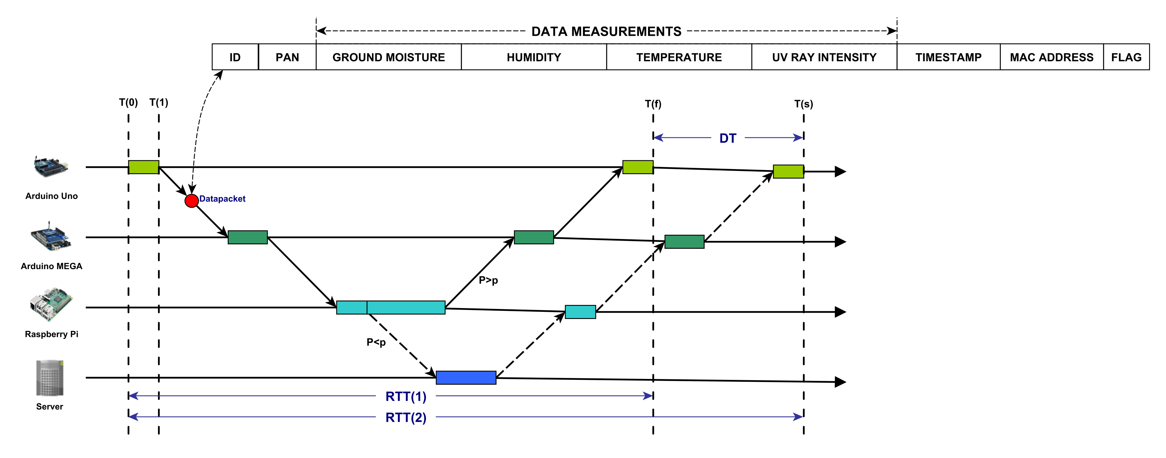
The data were sensed, timestamped, and encapsulated inside a data packet at regular intervals, which also contained information regarding the MAC address of the corresponding Arduino Uno. The data packet was then transmitted, based on the routing scheme of the ZigBee protocol, towards the sink node. The latter, upon reception, stored the data into its SD card, subsequently encapsulated inside the data packet the PAN id of the WSN, and then, forwarded the data packet to the appropriate fog device, which in turn based on a probability P, decided whether to compute the data locally or forward the data deeper into the cloud infrastructure (i.e., the remote server VM) through 3G. P is a system parameter that can be easily altered to mirror the necessity for lower response time, according to the farmers’ occasional needs.
Nevertheless, in both cases, i.e., the fog processing scenario or the cloud processing scenario, the data packet underwent the same data treatment, which resulted in a new data packet, containing the mean values for each measurement variable. The data packet then followed the opposite network path towards the appropriate Arduino Mega (based on the stored PAN id) and from there towards the Arduino Uno that initially sensed the data (based on the stored MAC address). This whole process is illustrated in
Figure 10, where the squares represent processing time and the arrows refer to the transmissions that take place. The complete structure of the data packets is also illustrated.
To further break down
Figure 10, at time
, an Arduino Uno node generated a new data packet, containing the newly obtained field measurements along with its MAC address, and timestamped it accordingly, before sending it at
to the Arduino Mega. Note again that the depicted process corresponded to the simplest case scenario, a full topology WSN, where all nodes communicated directly with the sink node. However, the same applied to complex multi-hop WSNs with the intervention of intermediate nodes. As already described, the Arduino Mega performed some processing to extract the data and store them into its SD card. It then forwarded the data to the overseeing fog device. The latter, upon reception, based on a probability
p, decided how to handle the data packet. As such, two cases were present.
In the first case, where (P as already mentioned was a system input parameter), the data were processed locally by extracting the data and computing their mean values, based on all similar data received up until that point from all nodes belonging to the same WSN. It then encapsulated the calculated values inside the data packet, overwriting the previous ones, and transmitted the data packet back to the correct Arduino Mega based on the PAN id. The Arduino Mega then read the MAC address stored inside the data packet and forwarded it to the corresponding Arduino Uno, which at that point read its local clock and calculated the total round trip time . Here, referred to the time that elapsed between data generation and the moment the Arduino Uno received and extracted the appropriate response from the cloud/fog infrastructure, i.e., .
On the contrary, in the second case, where , the data were processed remotely at the cloud server. Therefore, the data packet was initially transmitted from the fog device to the server VM through 3G, which then, similarly to the former case, computed the mean values for the data measurements. This process, however, due to the increased computational capabilities of the server, took lesser time. The data packet was then transmitted back to the fog device, which then, based on the encapsulated WSN PAN id, forwarded the data to the appropriate Arduino Mega. From there, the process was similar to the first case since the data packet was then transmitted to the corresponding Arduino Uno (based on the stored MAC address), which then calculated the for the specific data packet, i.e., .
Notice that the difference between the two s was considered an estimate of the performance advantage of the hybrid cloud/fog system versus a conventional cloud-only system since it was feasible with the employment of more fog functionality to achieve response time reduction, if there existed an emergency that required faster and more reliable WSN activity tracking (e.g., in the case of pest infestation in one of the monitored olive groves). The difference was calculated as: . Therefore, it followed that .
7. Evaluation
The current section procures experimental results regarding the utilization of the developed prototype system in the facilities of the Ionian University. The results report on the efficiency of the approach.
7.1. Response time Adjustability
The experimental prototype was initially put to the test to evaluate its performance in terms of latency, which is defined as the response time, i.e., the Arduino Uno devices’ (and eventually the farmers’) mean perceived round trip time () (as calculated in the previous section), which as already stated was considered to be the most important factor to achieve an acceptable degree of precision. The response time is plotted based on different values for the probability P, i.e., the possibility to process the data locally at the deployed fog network, which took values inside , incremented by at each experimental cycle, leading to eleven (11) different runs. Each experimental cycle lasted 30 min and was iterating through five (5) different scenarios regarding the system’s input parameter value for the time interval between the sensors’ reading rates, leading to a total of 55 experimental cycles. The experiment was then repeated during a different day, yielding the same attitude. The results are presented next, averaged over the two conducted experiments.
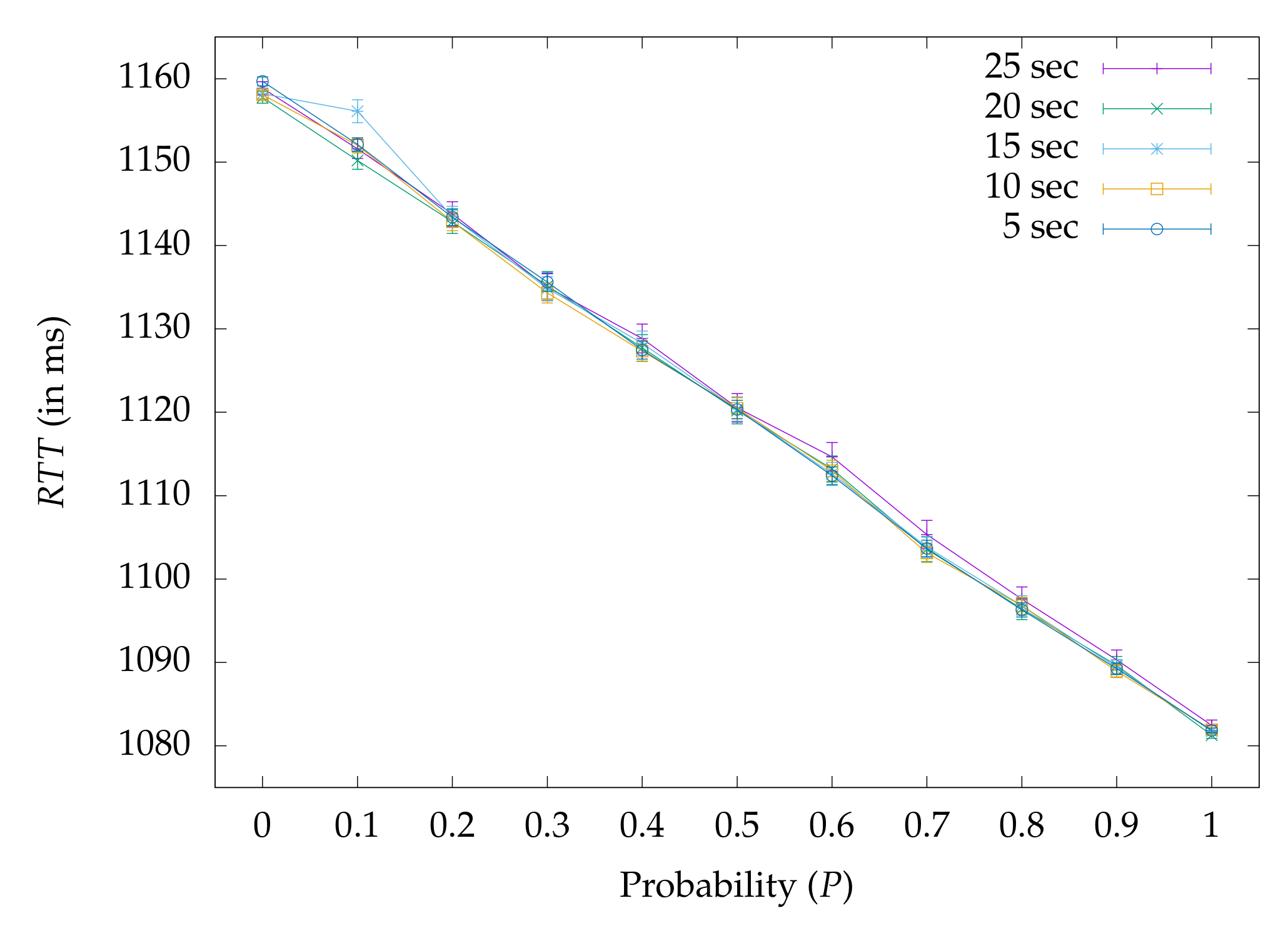
Starting from the average total perceived response time of the system,
Figure 11 illustrates the behavior of the system. As expected, the mean
degraded as more cloud tasks were offloaded to the Raspberry Pis by increasing the value of
P (in each consecutive scenario,
P was increased by
); ergo, the system’s mean
was continuously reduced as more functionality was pushed towards the underlying fog network. The depicted plot also encapsulates the resulted mean
for the two extreme values of
P, i.e., for
, where all processing took place remotely, and for
, during which all processing occurred locally. Additionally, for the case of the 25 s interval, the number of packets generated by the WSNs’ nodes was much less than the number of data packets generated during the 5 s interval scenario. This approach was followed to determine if higher reading rates affected the system’s overall behavior. However, as observed, no clear tendency could be derived by the reduction in the time interval regarding the mean
, which in all five depicted scenarios followed the same decaying attitude, leading to the result that the fog network successfully handled the incoming traffic.
Following,
Figure 12 further decomposes the previously described behavior by encapsulating the results of the approach, estimated again by the
value, as a function of the probability
P, through the scope of the fog devices (i.e., the three Raspberry Pis) for the minimum and maximum tested intervals, with 95% confidence interval bars. In all depicted circumstances, the results verified the expected outcome, mirroring the total system’s behavior. It is understandable that the Raspberry Pi with the highest workload due to more WSN connections according to
Table 4, i.e., Fog Device 1, would have a higher range of
values starting in both cases at around 1165 ms for
. This is explained by the fact that it had to iterate through more serial ports, collecting and subsequently processing more incoming data packets, whereas the Raspberry Pi with the fewest WSN connections, i.e., Fog Device 2, would have the lowest
range, respectively, starting for
at around 1155 ms.
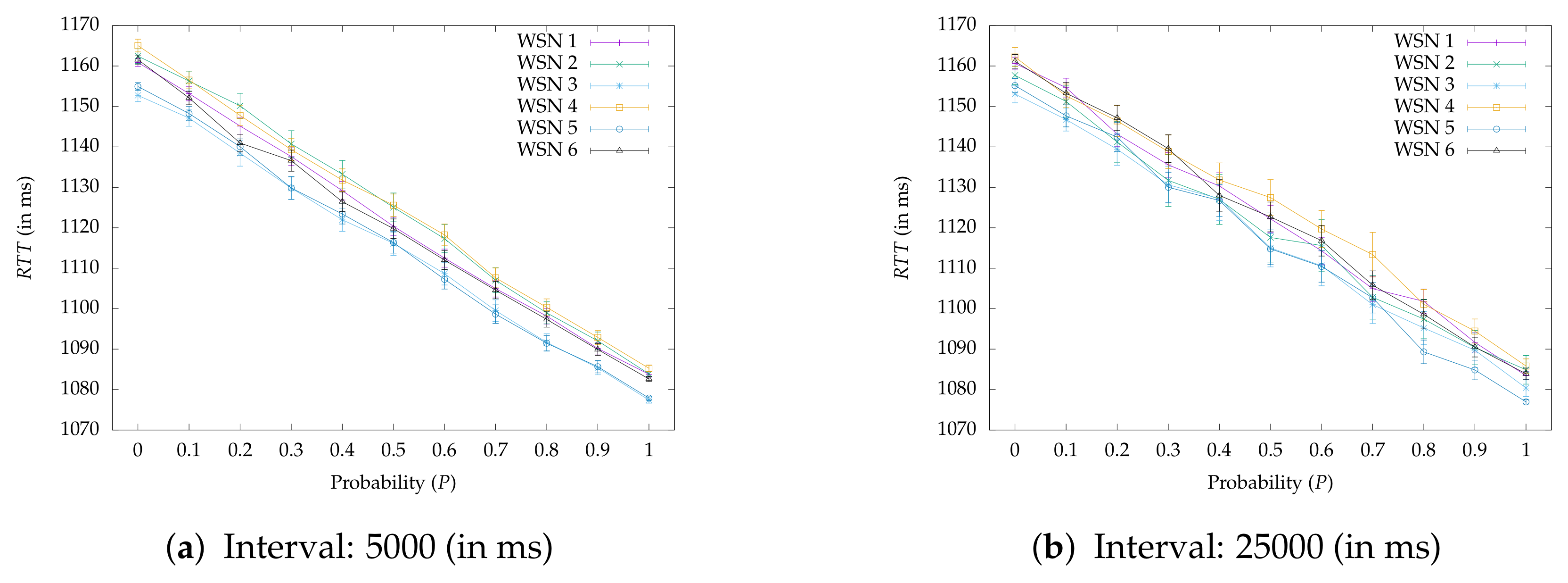
To strengthen even more the previous research findings,
Figure 13 deconstructs the fog device plots to the level of the involved WSNs, again based on the ids listed in
Table 4. As such, it reports on the farmer’s perceived average achieved response time, estimated by the mean
values from the perspective of each separate WSN used in the demo prototype, with 95% confidence interval bars. It is noteworthy that the depicted mean
s verified once more the effectiveness of the approach since all values steadily decayed as the probability
P rose for all WSN instances. In fact, it was assumed that in the best-case scenario, where no other delays were present due to server/fog overloading or network bottlenecks, the total
was directly proportional to the distance between the cloud server and the fog devices, the distance between the latter and the WSNs, as well as the speed of the transmission medium and the adopted communication protocol. Consequently, occasional
spikes in the depicted plots were purely attributed to potential time-processing fluctuations (mainly at the fog and cloud server sides) and delays incurred either by the CSMA/CA ZigBee protocol (at the WSN side) or other network factors at the time of experimentation.
The aforementioned experimentation results proved the efficiency of the proposed system architecture at meeting the requirements of the farmers for faster and more precise olive grove monitoring aiming at ensuring early notification in the case of an emergency. Notice again that a drawback, which was adopted intentionally for reasons of simplicity, referred to the fact that all presented experimental results corresponded to the simplest use case scenario, where all WSNs’ sensor nodes were located one hop away from the sink nodes; therefore, they were in range with one another and could directly communicate with each other. Nevertheless, the logic behind the system architecture was axiomatically the same for a system containing multi-hop WSNs; however, this should be further investigated, but is beyond the scope of the current paper.
Besides, it is also worth highlighting that in all experiments that took place, for , the system yielded the highest values for . This is important because it referred to the case where all data processing was facilitated solely in the remote cloud server. In other words, for , the system behavior fell into the conventional cloud-only approach, and therefore, it was derived that this was not the optimal configuration, since in all following experiments that involved the deployment of the fog network, the hybrid cloud/fog system outperformed the conventional cloud-only model, validating the claims of the paper.
On the other hand, regarding the case for , the system behavior fell into the fog-only approach, distributing the workload among various fog devices. This approach yielded the lowest s, since it was distance-dependent, bringing all cloud resources in close proximity to the end users, in this case the Arduino Uno devices and eventually the farmers. Although this approach showed the most promising results, nonetheless, it was not considered the optimal solution for future farming, which would require the successful correlation of multiple olive grove sources to assess the overall characteristics of the considered habitat. On the contrary, both the cloud and fog were complementary and interrelated, since in most cases, there must exist a centralized control to manage the system’s global operation in cases when one or more fog devices suddenly fail (e.g., due to exogenous factors) and the information flow must be redirected to other sources in the cloud. Moreover, central management was required to keep track of the overall health of the monitored olive groves or farmlands, especially when a farmer may own several geographically scattered acres of land and the generated data from all individual fog devices must be successfully correlated. However, these use case scenarios must be further explored in future work, which will concentrate on the strategic placement of the fog devices, as well as the adjustability of the system, with the goal of addressing extreme phenomena, which render the installed fog devices or WSN nodes incapable of further computation or even operation.
7.2. Load Balancing and Throughput
Although the previous experiments remarked on the effectiveness of the proposed system, nonetheless, a more practical application scenario was needed to highlight and better contextualize its conforming character. Thereafter, an experiment was executed to observe the effect that fog overloading had on the system and how the latter coped with the workload in terms of latency.
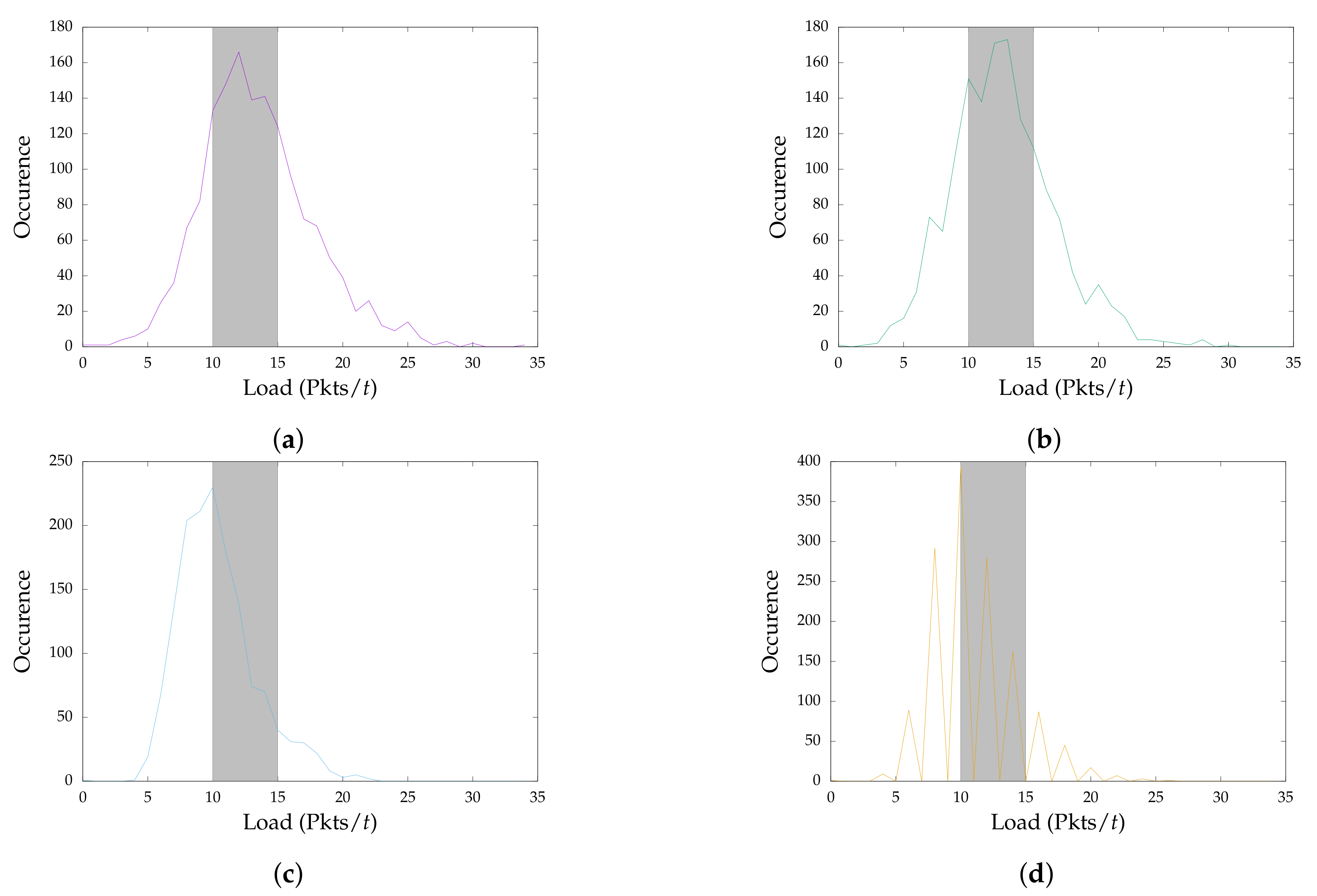
Two boundaries were chosen to drive the load balancing procedure. Notice that the load in the current paper was proportional to the number of packets received per time step t. Estimations about the load took place considering a time step of 30 s. The upper bound (i.e., 15 packets per t) indicated the point beyond which the fog devices became overwhelmed and functionality must be pushed towards the server. In comparison, the lower bound (i.e., 10 packets per t) defined the point below which the fog devices were underperforming, and so, they pulled functionality from the server to leverage the traffic burden. This load window was specifically chosen to be small to envision a better overview of the balancing process since in this way, the generated packet rate would hit the bounds frequently and the load evening events would be triggered often. In particular, when the data packet accumulation surpassed the upper bound, the corresponding fog device decided that it was time to push functionality towards the server and, therefore, decreased the probability P for the data packets to be processed locally. For every iteration of the time step t, where the upper bound was violated, the probability P decayed by 0.05. Alternatively, when the lower bound was infringed upon, similarly to the previous rule, the fog device recognized it was time to cut down on the server forwarding so as to free server resources, by increasing the probability P for the data packets to be processed locally. For every iteration of the time step t, where the upper bound was violated, an increment to the probability P by 0.05 occurred.
The experiment lasted around 13.5 h during which the sensory devices did not follow any particular patterns in their sensing process, but instead generated data at completely random intervals to produce fluctuations in the number of procured data packets per time step, as well as per fog device. The initial value for
P was set to one, i.e.,
, which then was adjusted based on the load balancing rules, as explained earlier.
Figure 14 illustrates the load balance achieved among the server and the fog devices. In all depicted cases, most of the load values were clustered around the grey zone [
10,
15], meeting the given constraints and proving that the fog devices were capable of successfully estimating their traffic load at each
t in order to make targeted adjustments to their operation and equilibrate the workload between them and the server. This would prove especially helpful in future real field deployments, which would require huge volumes of data handling, especially in cases of environmental hazards (e.g., fungi diseases, pest infestations, wildfire outbreaks, etc.) that require close timely field monitoring and high data packet generation rates, for the olive growers to detect their potential appearance early and prevent them by launching appropriate countermeasures. Notice that the spikes in
Figure 14d were purely attributed to the fewer number of sensory nodes, generating less traffic at their associated fog device.
On the other hand,
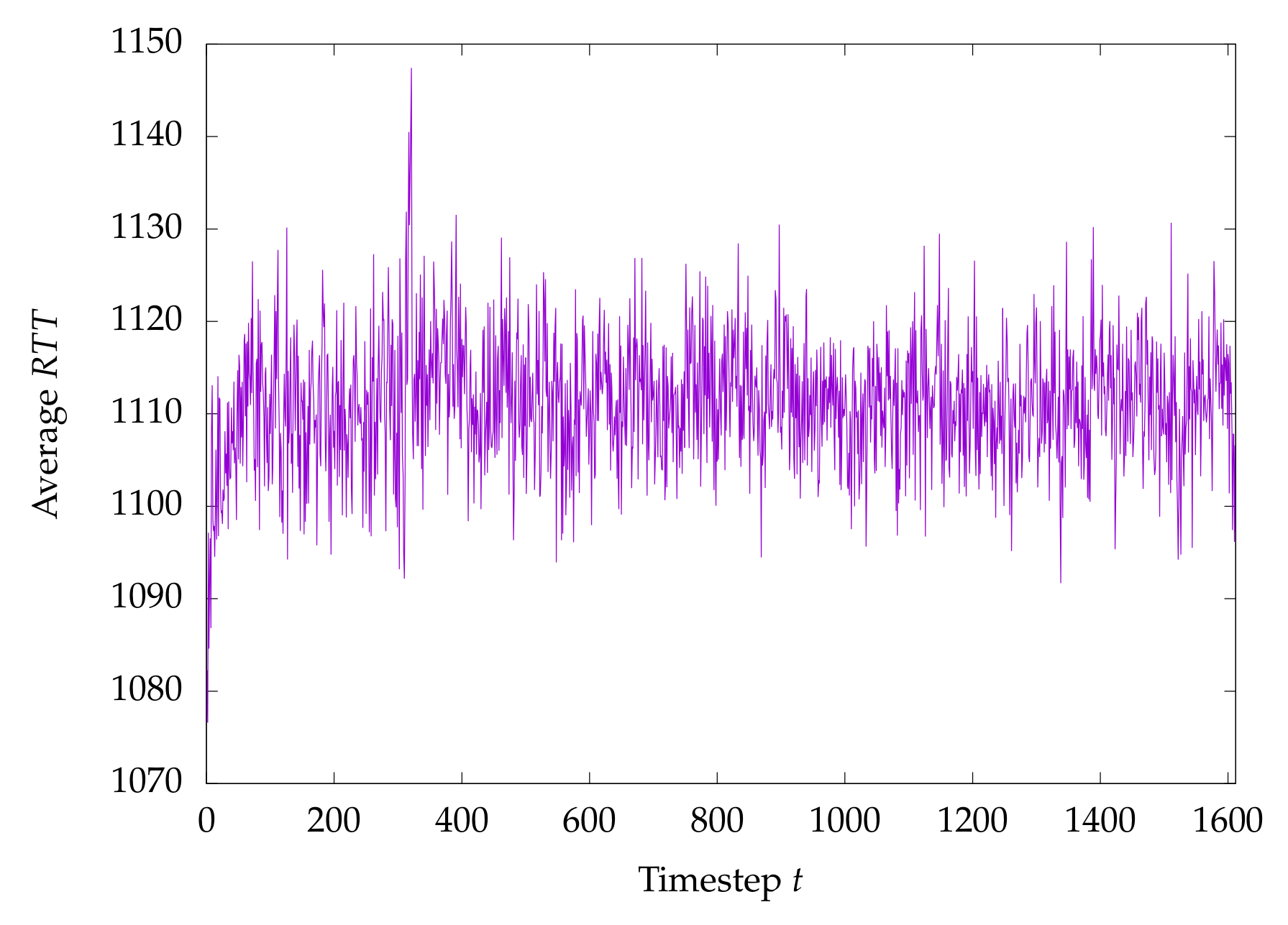
Figure 15 captures the system’s overall average
(in ms) as a function of time step
t during which the load at each fog device was estimated based on the previously explicated load boundary window. As observed, the
remained for the duration of the experiment relatively stable (around
ms). This could be explained by the load balancing occurring at each
t. By pushing/pulling functionality towards/from the cloud server, it was shown that the fog devices were able to maintain the network traffic and processing weighted between them and the server, ergo, constantly offering a rather stable response time, even during periods of high sensory data packet accumulation.
Lastly, it was considered important to highlight the efficiency and credibility of the system approach in terms of throughput. Throughput here was considered to be the percentage of successfully delivered data packets over the number of initially generated at the sensor nodes.
Figure 16 encapsulates the experimental results regarding the latter for each time step
t. Thereafter,
Figure 16a depicts the number of successfully retrieved data packets, whereas
Figure 16b presents the achieved system throughput (in %). It is noteworthy that in all time steps
t, even when a high data packet conglomeration rate appeared in the system, the throughput remained at high levels, approximating the average value of 95% (minimum 72% and maximum 100%). Any losses were ascribed to the underlying ZigBee/CSMA protocol retransmissions or to natural obstacles in the area of experimentation (e.g., furniture, walls, etc.) that affected the communication range of the sensory nodes. Although the throughput ranged in high percentages, it was understandable that in a large-scale deployment on olive groves, where the number of WSN nodes and distances between them would grow significantly, the data losses would potentially be graver. Nevertheless, this limitation could be sufficiently addressed through careful allocation of the sensory nodes and the strategic placement of the sink and fog nodes.
8. Conclusions and Future Work
The current work reported on the design, implementation, and deployment of a novel system architecture, examining a range of latency of stringent environmental factors for olive groves in Greece and specifically on Corfu Island. To achieve this, the architecture embedded low-cost, power-efficient, and highly configurable smart technologies from different ICT domains that included IoT solutions and WSN appliances, while in its core, it followed cloud/fog computing approaches.
Contrary to previous approaches, the three-layered architecture seamlessly integrated all the aforementioned technologies and emphasized the dynamic adaptability to network factors and field environmental agents that affected the system’s robust operation. In particular, the proposed approach utilized field deployment of sensors to form flexible WSNs that communicated with a main cloud infrastructure through the intervention of an intermediate fog computing network, constructed by smart microcontrollers, to offer the stakeholders the opportunity for almost real-time monitoring of their lands. The data produced could be easily accessed, since they were stored in appropriate forms across many system entities, and could be further employed to feed into specialized agricultural models, to procure instantaneous decision-making sequences regarding the health of the olive groves. Ergo, the essential contribution lied in the adjustable latency and load balancing capabilities, which were evaluated extensively through the creation of a robust prototype demo in the facilities of the Ionian University and a performance analysis across all involved system components. The experimental results captured the expected behavior and validated the effectiveness of the prototype in dealing with time-sensitive agricultural applications, procuring high throughput (around 95% on average). In all cases, the average response time was reduced with the intervention of the fog computing network. In fact, it was proven that as more functionality was pushed to the edges of the cloud and in closer proximity to the deployed WSNs, and eventually the farmers, the response time of the hybrid system was steadily improved, outperforming the cloud-only model, whilst keeping the load at optimum capacity both in the fog and cloud counterparts.
The presented work also reported on system limitations, the biggest barrier being the lack of a real large-scale olive grove deployment. Additionally, constraints relating to optimized energy consumption, nodes’ clock synchronization, and overall automation were also discussed. However, actions were taken in these directions through custom-designed elements that tackled these obstacles and offered the system flexibility and credibility. Nevertheless, future work will focus more intensively on these subjects as they are considered critical for the adoption of the proposed architecture, along with the experimentation on various network topologies, which also include multi-hop WSNs and different routing algorithms, which will enhance the data transmission process and locate the optimal placement for the nodes and the fog devices. Moreover, alternatives to the ZigBee communication protocol, like LoRa, must also be investigated, since the latter can significantly expand the coverage area.
Consequently, prior to field deployment, it was considered an important step to investigate more deeply the implications of the proposed system in dealing with other agricultural dangers. To this end, alternative sensor modules must also be explored and validated in regards to efficiency and throughput, such as images or videos captured by IoT cameras installed in the field of study or soil pH trackers. The lack of standardization in the agricultural IoT domain would drive the development operations, with the aim of gaining knowledge around the optimal setup and configuration for addressing these challenges. The system will then be installed at full scale in real olive groves, where its activity and operation will be extensively recorded and documented under different conditions and environmental parameters. Note that a dataset construction is already underway; however, detailed analysis is yet to be undertaken in order to procure concrete results for the olive growers. However, a milestone in this process will include the autonomous and automatic adjustability of the architecture’s behavior to counterbalance implications and hazards imposed by system failures in one or more of the system’s entities, e.g., the fog devices. Lastly, a web interface will be created, which will remotely allow the management and overseeing of the system through various platforms.
In concluding the paper, it is clear that the proposed architecture and implementation is very promising and holds huge potential for smart agriculture, and farmers alike, but still requires further research and understanding. Future guidelines include, but are not limited to, behavior optimization to modify the system’s characteristics dynamically to deal with various agricultural aspects, other than olive grove monitoring, but also to support emerging technologies, comply with the future 5G standards, and transparently “marry” and bridge the gap among different agricultural scientific disciplines and environmental domains. Besides, the proposed system is inherently generic in nature and can easily adapt to such changes, offering a multitude of benefits to the involved parties.

 ,
, 


