Deep Learning Application in Plant Stress Imaging: A Review


1
Department of Biological Systems Engineering, Center for Precision and Automated Agricultural Systems, Washington State University, Prosser, WA 99350, USA
2
School of Life Science and Engineering, Southwest University of Science and Technology, Mianyang 621010, China
3
College of Information and Technology, JiLin Agricultural University, Changchun 130118, China
*
Authors to whom correspondence should be addressed.
AgriEngineering 2020, 2(3), 430-446; https://0-doi-org.brum.beds.ac.uk/10.3390/agriengineering2030029
Submission received: 19 May 2020
/
Revised: 27 June 2020
/
Accepted: 7 July 2020
/
Published: 14 July 2020
(This article belongs to the Special Issue Precision Agriculture Technologies for Management of Plant Diseases)
Abstract
:Plant stress is one of major issues that cause significant economic loss for growers. The labor-intensive conventional methods for identifying the stressed plants constrain their applications. To address this issue, rapid methods are in urgent needs. Developments of advanced sensing and machine learning techniques trigger revolutions for precision agriculture based on deep learning and big data. In this paper, we reviewed the latest deep learning approaches pertinent to the image analysis of crop stress diagnosis. We compiled the current sensor tools and deep learning principles involved in plant stress phenotyping. In addition, we reviewed a variety of deep learning applications/functions with plant stress imaging, including classification, object detection, and segmentation, of which are closely intertwined. Furthermore, we summarized and discussed the current challenges and future development avenues in plant phenotyping.
1. Plant Stress and Sensors
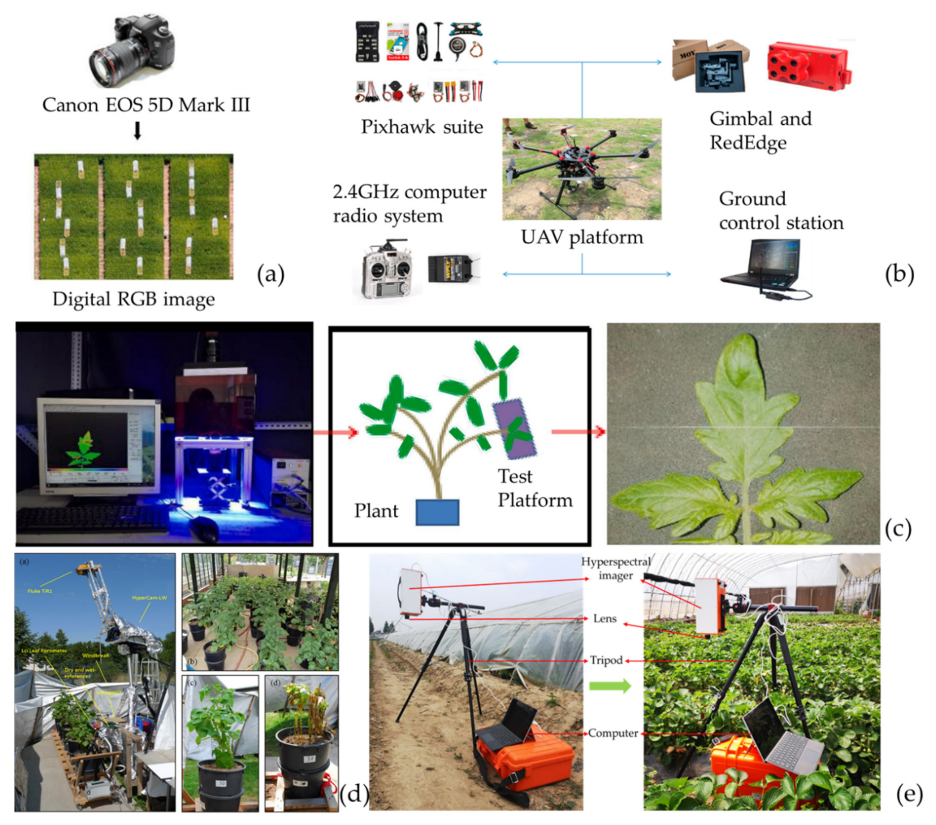
Plant stress is one of the major threats to crops causing significant reduction of crop yield and quality [1]. The detection and diagnosis of the plant stress is urgently needed for rapid and robust application of precision agriculture in crop measurement. Presently, intensive studies focus on developing optical imaging methods for plant disease detection. Different from the conventional methods using the visual scoring, optical imaging is advanced to measure changes caused by abiotic or biotic stressors in the plant physiology rapidly and without contact. In general, the common imaging technologies have been employed for detecting the crop stress, including digital, fluorescence, thermography, LIDAR, multispectral, and hyperspectral imaging techniques [2]. The common optical sensors used for plant stress detection are shown in Figure 1.
Digital imaging sensors acquire the visible range of wavelengths, i.e., RGB colored images with red, blue, and green channels to detect plant diseases. Such images provide physical attributes of the plants, such as canopy vigor, leaf color, leaf texture, size, and shape information [8]. Color and texture features are important for identifying the characteristic difference between healthy and symptomatic plants. Frequently used color features are RGB, LAB, YCBCR, and HSV spaces [9]. Additionally, contrast, homogeneity, dissimilarity, energy, and entropy features of images are descriptive facets of texture [10]. In other words, quantitative diagnosis features for identifying the symptomatic and healthy plants have been collected in these images.
Thermal imaging sensors obtain infrared radiating images ranging from 8 to 12 μm, which are often applied for predicting plant temperatures. Under the infection, the temperature of infected plant tissues varies and related to the impacts caused by pathogens. The temperature variance, other the hand, appears with a counter-effect on transpiration rate [11]. In other words, stress from the infection trigger both transpiration rate decrease and leaf temperature increase, resulting in stomatal closure in plants. In turn, based on these alterations, thermal imaging sensors could identify the infection diseases. Each pixel of the thermal image represents the temperature value of the object, which is expressed in manners of false color. In plant disease detection, the thermal sensor could be mounted to ground automated vehicles (GAV) and unmanned aerial vehicles (UAV).
Fluorescence imaging sensors are often utilized to identify variations of plant photosynthetic activity [12]. The differences of stressed and healthy leaves will be expressed in the differences of photosynthetic activities, which will be assessed by the photosynthetic electron transform using the fluorescence imaging sensor with an LED or laser illumination. For normal cases, 685 nm is the wavelength at which chlorophyll fluorescence is emitted from photo-system II (PSII). The stressed plants could change the patterns of chlorophyll fluorescence emission, which could be reflected and observed in the fluorescence imaging [13].
Based on the number of spectral bands in the optical sensing technologies, sensors contain 3–10 spectral bands are named multispectral imaging sensors. The multispectral imaging sensors normally extract a few or a stack of images from the visible to near-infrared spectrum [14]. Plant stress often causes an increase in visible reflectance, with a decrease in chlorophyll and absorption of visible light. Additionally, reduced near infrared (NIR) reflectance will happen due to changes of the leaf tissue. Thus, the most used band channels are green, red, red-edge and NIR. Multispectral imaging sensor combined with drones have been applied broadly in remote sensing for plant disease detection [15], while this type of sensors is limited to a few spectral bands and sometimes cannot quantify the diseased plants severity.
Despite many successful studies having been applied to crop stress detection using cheap passive imagery sensors, i.e., digital and near infrared (NIR), most of the applications require fast image processing and computational algorithms for image analysis. Among the image analysis techniques, supervised methods have been popular with training data being used to develop a system. Such methods include shape segmentation, feature extraction, and classifiers for stress diagnosis. In addition, machine learning algorithms search for the optimal decision boundary in the feature space with high dimensionality, which provides the basis for many available image analysis systems [16].
For improving the image analysis systems, deep learning has played a key role. Deep neural networks have many layers which transform input images to outputs (i.e., healthy or stressed) with learning deep features. The most applied networks are convolutional neural networks (CNNs) in crop image analysis. CNNs consist of dozens or hundreds of layers that process the images with convolution filters with a respective small size of batches [17]. Despite such initial successes, CNNs cannot collect momentum without the advances in core computing systems and deep convolutional networks become the current focus. In agriculture, deep learning shows accepted performance considering accuracy and efficiency based on large datasets. To build precise classifiers for improving plant disease diagnosis, the PlantVillage project (https://plantvillage.psu.edu/posts/6948-plantvillage-dataset-download) has obtained a large number of images of healthy and diseased crops for free [18]. Combined with the big data, deep learning has been put forwarded as the future promising method in plant phenotyping [19]. For example, CNNs can effectively detect and diagnose plant diseases [20] and classify plant fruits in the field [21]. The promising results promote studies carrying out other phenotyping tasks using deep learning, such as leaf morphological classification [22]. Thus, we read many references about the utilization of deep learning in image-based crop stress detection. Summarizing, with this paper we aim to:
- State the principle of deep learning in the application for crop stress diagnosis based on images.
- Search for the challenges of deep learning in crop stress imaging.
- Highlight the future directions that could be helpful for circumventing the challenges in plant phenotyping tasks.
2. Deep Learning Principle
2.1. Machine Learning
Machine learning is a subset of artificial intelligence which is used to operate specific tasks by computer systems [23]. In general, it is split into supervised and unsupervised learning methods. Supervised learning methods are expressed with an input matrix of independent x and dependent y variables. This dependent variable of y has few formats, varying based on solving problems. For classification issues, y is usually a scalar for representing the category labels, and it is a vector containing continuous values under regression [24]. Under segmented learning conditions, y is sometimes the ground truth label image [25]. Supervised learning methods often aim to find optimal model parameters, which could predict the data to the greatest extent based on the loss function.
Unsupervised learning methods operate data processing without dependent labels and aim to search for patterns (e.g., latent variables). Common unsupervised learning methods include principal component analysis (PCA), k-nearest neighbors clustering, and T-distributed stochastic neighbor embedding clustering [26]. Unsupervised training usually uses many different loss functions to process, such as reconstructing the loss function. The model must learn to reconstruct the loss function in a smaller dimension to reconstruct the input data [27].
2.2. Neural Network
A neural network is built to recognize patterns and provides the basis for most deep learning algorithms [28]. A neural network contains nodes that integrate input data with a set of coefficients and weights with amplify or dampen the input for learning the assigned tasks, e.g., the common activation function α and parameters , here, w represents the weights and β represents the biases. An activation function is normally followed by an elemental nonlinear factor/coefficient σ, as a transfer function, as shown in Equation (1) [28]:
Sigmoidal and hyperbolic tangent functions are the common transfer functions for neural networks. The multilayer perceptron (MLP) is the most popular one in traditional neural networks, with few conversion layers [28]:
where is a matrix containing rows that is related with activation k in the output, and L is the final layer. The so-called hidden layers are the layers between input and output layers. A neural network with many layers is often called deep neural network (DNN), thence deep learning. The activation of the last layer is mapped to distribution on the class P (y|x; Θ) through a softmax function [28]:
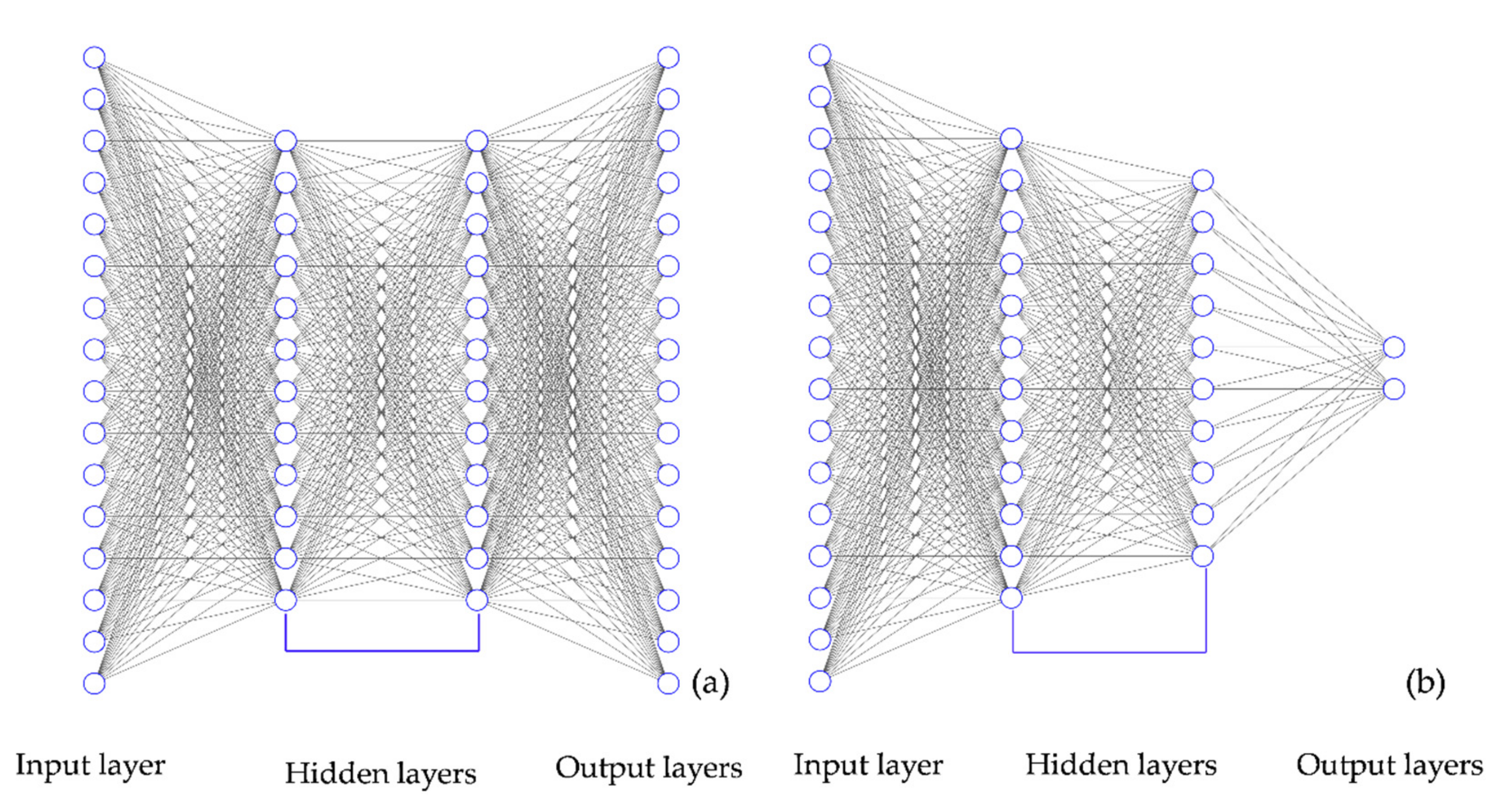
where is the weight vector associated with class i to the output node. The typical diagram of deep neural network MLP is shown in Figure 2.
Currently, stochastic gradient descent (SGD) is the famous method for fitting the parameter Θ to process a small population dataset. With SGD, a small batch is employed in each gradient and maximum likelihood optimization is used to minimize the negative impact of the log-likelihood. It tracks the log loss for a binary classification task and the softmax loss for multiclass classification. A disadvantage of this method is that it usually does not directly optimize the quantity of interest [28].
DNN became popular in 2016, when it performed layer-by-layer training (pre-training) in an unsupervised manner, and then supervised and fine-tuned the stacked network to obtain good performance. Such a DNN architecture includes a stacked autoencoder (SAE) and a deep summary network (DBN). However, such methods are often complex, which need a great deal of engineering to obtain acceptable results [28,29]. Recently, end-to-end training has been conducted on popular architectures in a supervised manner by streamlining the training procedure. The common architectures are CNN and recurrent neural network (RNN) [30,31]. CNN has been widely used for image analysis, and RNN is becoming more and more popular.
2.3. Convolutional Neural Network
The main difference between MLP and CNN is reflected in two aspects. First, weights of the CNN architecture are shared with a network when the architecture operates convolutions on the input image [32]. In this way, separate detector learning is not required for the same object appearing at different locations in the image. As a result, the network is equally variable in the translation of input images. In addition, the number of parameters to be learned is reduced.
During CNN training, the input images are convolved with a set of K kernels and biases in the convolution layer, yielding a new feature map . Such features are exposed to a nonlinear transformation parameter σ and such process would repeat for each respective convolutional layer l [32]:
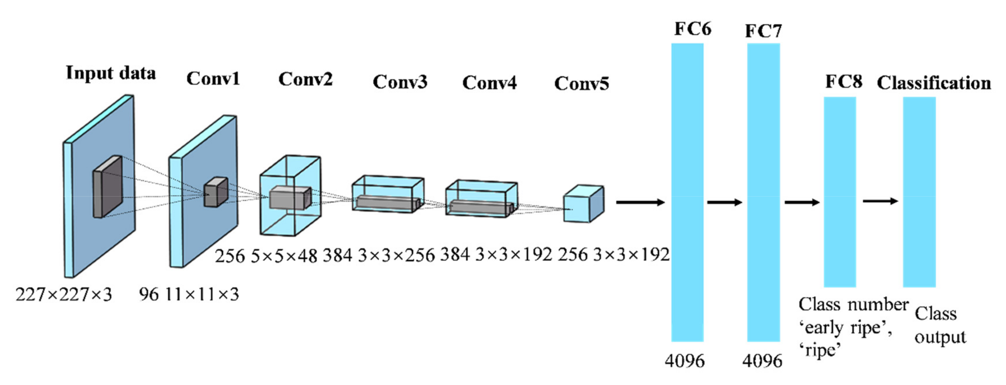
Second, the main difference between MLP and CNN is the pooling layer. In such layers, the pixels of the neighborhood are added based on the permutation invariant function in CNN. This may prompt a certain amount of rendering invariance [33]. Then, the fully connected layers are usually added with constant weights after convolutional processing. Then, the softmax function is used to provide activation information in the last layer, resulting in a category assignment. A typical CNN architecture is shown in Figure 3 for identifying the ripeness of strawberry based on hyperspectral imagery [34].
2.4. CNN Architecture
CNN normally uses a 2D image as input, with a format of m × n × 3 (m × n × 1 for greyscale images), where m and n are the respective image height and width, and 3 is the number of image channels. The CNN architecture often contains a few different layers, including convolutional layers, pooling layers, and fully connected layers. The convolutional and pooling layers are initial layers. A set of convolutional kernels (also called filters) is used for each layer performing multiple transformations. The convolution operations extract the associated features from small slices divided from the full image. Each kernel is applied to the input slice and the output of each kernel is applied to non-linear processing units, making it capable of learning abstraction and embedding non-linearity in the feature space [35]. The non-linear processing provides different patterns of activations corresponding to different responses, which helps learn the semantic differences over the full image. Then, the subsampling is applied to the output of non-linear processing, with summarizing the results and making the input insensitive to the geometric deformation [36]. The CNN architecture has been applied to many aspects, including classification, segmentation, and object detection, etc.
2.4.1. Classification Architectures
Among the pre-trained networks, AlexNet is commonly used for images classification, which is relatively simple with five convolutional layers. The activation function of AlexNet is the hyperbolic tangent, which is the most common choice in CNNs [37]. Then, the deep pre-trained networks appeared, such as the VGG19 with 19 deep layers, winning the ImageNet challenge of 2014 [38]. These deeper networks use smaller stacked kernels and have lower memory during inference, which improves the performance of mobile computing devices, such as smartphones [39]. Later, in 2015, the ResNet architecture won the ImageNet challenge and was made up of the ResNet blocks. The residual blocks learn the residuals and pre-processes the learning mapping for each layer, thereby providing effective training performance for deeper architectures. Szegedy et al. (2016) developed a 22-layer neural network referred as GoogLeNet, which employed the inception blocks [40]. The advantage of using the inception blocks is that it could increase the training process efficiency while decreasing the number of parameters. The performance on ImageNet reached saturation after 2014 and crediting the better performance to the more complex architectures is biased. On the other hand, it is not necessary to perform plant stress detection with the deeper networks, providing a lower memory footprint. Therefore, AlexNet or other relatively simple methods, such as VGG16, are still practical for crop stress images.
2.4.2. Segmentation Architectures
Segmentation is important in crop stress image analysis. The pixel in the image could be classified by the CNN and the classified pixel could be presented with patches that extracted from neighboring pixels [41]. The disadvantage of this method is that the input patches overlap, and the same convolution is repeatedly calculated. Fortunately, the linear operators (convolution and dot product) can be written as convolutions [42]. With a fully connected layer, a CNN can have a larger input image than the trained image and can generate a likelihood map instead of the output of a pixel. Then, such a full convolutional network can be effectively applied to the full input image.
2.5. Hardware and Software
The dramatic increase of deep learning applications could be due to the widespread development of GPUs [43]. GPU computing started when NVIDIA launched CUDA (Computing Unified Device Architecture) and AMD launched Stream. The GPU is a highly parallel computing engine which offers a great advantage compared with a central processing unit (CPU). The Open Computing Language (OpenCL) unifies different GPU general computing application programming interface (API) implementations and provides a framework that can be used to write programs that execute on heterogeneous platforms composed of a CPU and GPU. With the hardware, deep learning on the GPU is much faster than on the CPU [44].
Open source software packages also promote the development and application of deep learning. These software packages allow users to operate the computing at a high level without having to worry about efficient implementation. By far the most popular packages include:
Caffé, which offers C++ and python interfaces, developed by graduate students at UC Berkeley AI Research.
TensorFlow, which provides C++ and python interfaces, developed by Google Brain team.
Theano, which provides a python interface, developed by MILA lab in Montreal.
PyTorch, which provides C++ and python interface, developed by Facebook’s AI Research lab.
3. Applications of Deep Learning in Plant Stress Imaging
3.1. Classification
Deep learning has been applied successfully in plant phenotyping combined with various sensors and specific tasks, including harvesting crop counting, weed control, and crop stress detection [17,45,46,47]. Regarding crop stress detection, with various specific tasks, the image analysis methods are often varying among classification, segmentation, and object detection in crop stress detection combined with various sensors (Figure 4). Image classification is one of the earliest areas where deep learning contributed significantly to the analysis of plant stress images. In crop stress image classification, one or more images are usually used as input data, and a diagnostic decision is used as output (e.g., healthy or diseased). In this case, each diagnosis is a sample, and the size of the dataset is usually smaller compared to computer vision (thousands or millions of samples). Therefore, for such applications, the transfer learning should be popular for researchers. Transfer learning essentially uses pre-trained networks to try to meet the needs of deep network training on large datasets. At present, two transfer learning methods are commonly applied: (1) the specific pre-trained network is directly applied in images processing, and (2) fine-tuning the specified pre-trained network for the aiming objective images. Another benefit of the former strategy is that training a deep network is not necessary, making it easy to insert the extracted features into existing image analysis pipelines. However, it is still a challenge to find the best strategy. Barbedo (2019) used a CNN to classify individual lesions and spots on plant leaves instead of considering the entire leaf [45]. This identified multiple diseases that affect the same leaf. The accuracy obtained using this method was, on average, 12% higher than that obtained using the original image. While proper symptom segmentation is still required manually, preventing full automation. Also, in this paper, the authors applied deep learning to detect the individual lesions and spots for 14 plant species. Specifically, this study used a pre-trained GoogLeNet CNN for training the models. The images were split into two groups for addressing different objectives. The first group was aimed to image classification, to identify the origin of the observed symptom, while the second one was for object detection, which was to identify disease areas amidst healthy tissue and to determine if subsequent classification was conducted or not. The results showed that accuracies obtained using this approach were, in average, 12% higher than those achieved using the original images. The accuracies were higher than 75% for all the considered conditions or number of detected diseases, while the author also claimed that the resized input images for pre-trained neural network were not as advantageous as the original images under certain conditions. Other studies that applied the deep learning into the crop stress image classification are shown in Table 1.
3.2. Segmentation
Segmentation is used to identify the set of pixels or contours that make up the target object [70]. Segmentation is a common topic in papers applying deep learning to plant disease imaging. Various methods have been applied to segmentation, such as developing unique segmentation architectures based on CNNs and application of RNNs. The popular segmentation CNN architectures include U-Net and Mask R-CNN [71]. U-Net was investigated in biomedical image segmentation firstly [72], which was built upon a fully convolutional network (FCN). FCN is to provide one contracting network by continuous layers in which pooling layers are substituted by up-sampling operators. The continuous layer would learn to gather a more precise output, with an increase of the resolution of the output. U-Net is symmetric, that is, it has the same number of up-sampling and down-sampling layers. The skip connections in U-Net use a concatenation operator between the up-sampling and down-sampling layers [73]. This method connects the features in the contact path and the extension path. This means that the entire image is enabled to be processed forward through U-Net to directly generate a segmentation mapping. In this way, U-Net could consider the entire image, which make it more advanced than the patch-based CNN. Furthermore, Çiçek et al. (2016) built one 3D U-Net segmentation by replacing all 2D operations with their 3D counterparts [74]. Lin et al. (2019) applied a U-Net CNN to segment and detect cucumber powdery mildew-infected cucumber leaves obtained by an RGB sensor [46]. In this study, since the powdery mildew-infected pixels were less than that of non-infected pixels, the authors proposed binary cross entropy loss function to magnify the loss value of the powdery mildew-infected pixels by 10 times. The results showed that the semantic segmentation CNN model achieved an average pixel accuracy of 96.08% for segmenting the diseased powdery mildew on cucumber leaf images. It was still challenging to apply such deep neural network in field conditions. Different applications of deep learning into the crop stress image segmentation are summarized in Table 2.
R-CNN combines rectangular region proposals with CNN features. Generally, R-CNN includes two-stage detection procedures. Firstly, the algorithm detects subset regions of an image which may contain an object and extracts CNN features from the region proposals. Then the object in each region is classified. R-CNN takes a large amount of training of the deep neural network when there are 2000 or more region proposals per image that need to be classified. Meanwhile, there is no learning procedure at the first searching stage as the selective search algorithm is fixed. As a result, it may lead to tricky candidate region proposals being generated [80,81]. During R-CNN processing, the region proposals need to be cropped and resized, while the Faster R-CNN detector processes the entire image. Thus, Faster R-CNN can be applied for real-time object detection. Additionally, Faster R-CNN is the backbone of Mask R-CNN. Faster R-CNN includes two outputs, that is, a class label and a bounding-box offset. A third branch is added to mask R-CNN upon faster R-CNN architecture, which outputs the object mask [71]. In addition, Mask R-CNN is one of the instance segmentation algorithms which produce a mask that uses color or grayscale values to identify pixels belonging to the same object. Except to feed the feature map to the region proposal network and the classifier, Mask R-CNN uses a feature map to predict a binary mask for the object inside the bounding box.
3.3. Object Detection
Object detection is a key part in imaging diagnosis and one of the most laborious tasks. Typically, the task involves locating and identifying objects throughout the image [82]. For a long time, the research goal of computer vision was to automatically detect objects, for improving detection accuracy, and reducing labor. The object detection based on deep learning uses CNN for pixel classification and then applies some post-processing to obtain object candidates [81,82,83]. Since the image classification is to classify each pixel in the image, which is basically equal to object classification, thereby the CNN architectures of segmentation are alike to those for the classification task, while the image labels imbalance, hard negative detecting, and efficient processing image pixels etc., still remain as the challenging issues to be addressed for object detection. Fuentes et al., (2017) applied Faster R-CNN and a VGG-16 detector to recognize tomato plant diseases and pests [55]. Diseases and pests could be identified using the bounding-box and score for each class being shown on each infected leaf. That is, the detection method provides a solution for detecting the class and location of diseases in tomato plants practically. R-CNN and Faster R-CNN have been applied to object detection as well, using the regions in the image to locate the object. Recently, the YOLO algorithm has often been applied for object detection, which uses a single convolutional network to predict the bounding boxes and classify such boxes [84]. The YOLO algorithm divides the image into an M × M grid, then m (m<M) bounding boxes are taken within each of the grids. The network yields a class probability for each bounding box. When the bounding boxes have higher class probability than a threshold value, they would be selected and applied for locating the objects in the image. The limitation of the YOLO network is that it sometimes cannot identify small objects in the images [84]. Singh et al. (2020) applied Faster R-CNN with an InceptionResnetV2 model and a MobileNet model on PlantVillage datasets to detect plant disease, which included 2598 images from 13 plants and over 17 diseases [85]. Other applications for object detection are summarized in Table 3.
4. Unique Challenges in Plant Stress Based on Imagery
Noncontact plant stress detection has been conducted on different application scales, i.e., laboratory, ground-based, and UAV. Additionally, the modality has been operated based on a variety of sensors, such as digital, thermal, multispectral, and hyperspectral imagery, with different numbers of spectral channels, from three to hundreds. Such sensors could monitor the size, shape, and structural features or crops based on the external views obtained from digital cameras. The digital sensors could be easily operated under the natural light environment. Hyperspectral imaging sensors could obtain the inside spectral signatures beyond the visible wavelength range which could reflect the healthy crop conditions in a wide range of spectra, while most of the commercial hyperspectral imaging sensors could only work in laboratory with controlled light conditions at present. On the other hand, the wind will make the crops move around. In general, for image acquisition, it is still challenging for field work.
Further, the crops are not static: the physiological properties change with their growth. Especially for biotic stress infected crops, the fungi or viruses in the crops have great impacts on the physiological changes. It will be difficult to detect the stress at an early stage without symptoms showing based on image analysis. Further, for the application of deep learning-assisted image analysis, a lack of datasets is a major obstacle as well. At present, the available open source images are mainly from the PlantVillage dataset. On the other hand, one significant challenge is that of ground-truth labelling, which is hugely laborious. The Amazon SageMaker Ground Truth provides a service for managing the labelling, including two features. One is annotation consolidation, which combines different people’s annotation task results into one high-fidelity label. The second one is automated data labeling, which utilizes machine learning to label portions of the provided data automatically.
Moreover, to detect crop stress, the classification and segmentation are often used as binary tasks, i.e., healthy versus infected, target infected area versus background. However, since these two categories can be highly heterogeneous, this is usually a general simplification. For instance, the samples of the healthy class mainly consist of completely healthy objects but also rarely few objects showing early stresses. This could lead to classifiers that are able to exclude the healthy samples but cannot identify the few rare ones. The strategy for this case is to make a deep learning system with multiclass by giving it detailed annotations of all possible classes. Meanwhile, the within-class variance from images may reduce the sensitivity of the deep learning system. However, the between-classes variance from a dataset that may not be generalized to every image, such as the different severity of disease images, can obtain a pseudo-deep learning training architecture in one certain experiment, but obstruct the usefulness of its broad application to practical decision-making unless the nature of this dataset is precisely understood. Parameter optimization of the deep learning training models, i.e., batch size, learning rate, dropout rate, etc., is a remaining challenge as well. There is currently no exact method to achieve the best combinations of hyperparameters, which is often operated empirically, even though Bayesian optimization has been put forwarded.
5. Outlook
Deep learning has been applied successfully in plant stress (i.e., abiotic, and biotic stress) detection even though it still has many challenges. Most of the papers we have reviewed are based on the 2D images for symptomatic stages, for example the digital and greyscale images. Such images could be enabled to operate in the deep transfer learning architecture, such as Alexnet, VGG, GoogleNet, while such pre-trained transfer networks could not be applied to the 3D datasets, such as hyperspectral images, which are more sensitive to detecting the early-infected plants. In the future, deep neural networks that can be used for 3D images should be the focus and early detections of plant disease is pivotal to the precision disease management, especially for diseases without therapy using pesticide. On the other hand, many tasks in plant stress detection analysis could be granted, such as classification, and such a strategy may not be always optimal since it probably requires some post-processing, such as segmentation. Further, semi-supervised and unsupervised deep learning are worthy of being exploratory in the application of plant stress detection, though most of studies are based on supervised approaches. The advantage of unsupervised methods is that the networks training process could be operated without the ground truth labels. The unsupervised approach for detecting the plant stress are generative adversarial networks (GANs) [90], while another common unsupervised approach, i.e., variational autoencoders (VAEs), is rarely applied for crop disease diagnosis yet based on our knowledge [91]. Further, deep learning has been applied for other objectives in agricultural imaging, e.g., crop load estimation and harvesting, while image reconstruction remains unexplored, especially for LiDAR point cloud data. In general, deep learning has provided promising results in plant stress detection, which could accelerate the development of precision agriculture with the extension of field application.
Author Contributions
Conceptualization, Z.G., Y.X.; Supervision, W.Z.; Visualization, Z.L. (Zhongwei Luo), Z.L. (Zhenzhen Lv); Writing—Original Draft Preparation, Z.G.; Writing—Review & Editing, Z.G. and W.Z.; All authors have read and agreed to the published version of the manuscript.
Funding
This research was funded by [National Natural Science Foundation of China] grant number [31801625]; [Applied Basic Research Program of Science and Technology Department of Sichuan Province] grant number [2019YJ0444]; [Program of Key Laboratory of Modern Agricultural Equipment and Technology, Ministry of Education] grant number [JNZ201919], and [Longshan Academic Talent Research Supporting Program of SWUST] grant number [17LZX546].
Conflicts of Interest
The authors declare no conflict of interest.
References
- Cattivelli, L.; Rizza, F.; Badeck, F.W.; Mazzucotelli, E.; Mastrangelo, A.M.; Francia, E.; Stanca, A.M. Drought tolerance improvement in crop plants: An integrated view from breeding to genomics. Field Crop. Res. 2008, 105, 1–14. [Google Scholar] [CrossRef]
- Araus, J.L.; Cairns, J.E. Field high-throughput phenotyping: The new crop breeding frontier. Trends Plant Sci. 2014, 19, 52–61. [Google Scholar] [CrossRef] [PubMed]
- Elazab, A.; Ordóñez, R.A.; Savin, R.; Slafer, G.A.; Araus, J.L. Detecting interactive effects of N fertilization and heat stress on maize productivity by remote sensing techniques. Eur. J. Agron. 2016, 73, 11–24. [Google Scholar] [CrossRef]
- Zhang, L.; Zhang, H.; Niu, Y.; Han, W. Mapping maize water stress based on UAV multispectral remote sensing. Remote Sens. 2019, 11, 605. [Google Scholar] [CrossRef] [Green Version]
- Dong, Z.; Men, Y.; Liu, Z.; Li, J.; Ji, J. Application of chlorophyll fluorescence imaging technique in analysis and detection of chilling injury of tomato seedlings. Comput. Electron. Agric. 2020, 168, 105109. [Google Scholar] [CrossRef]
- Gerhards, M.; Rock, G.; Schlerf, M.; Udelhoven, T. Water stress detection in potato plants using leaf temperature, emissivity, and reflectance. Int. J. Appl. Earth Obs. Geoinf. 2016, 53, 27–39. [Google Scholar] [CrossRef]
- Kim, Y.; Glenn, D.M.; Park, J.; Ngugi, H.K.; Lehman, B.L. Hyperspectral image analysis for water stress detection of apple trees. Comput. Electron. Agric. 2011, 77, 155–160. [Google Scholar] [CrossRef]
- Mahlein, A.K. Plant disease detection by imaging sensors–parallels and specific demands for precision agriculture and plant phenotyping. Plant Dis. 2016, 100, 241–251. [Google Scholar] [CrossRef] [Green Version]
- Barbedo, J.G.A. Digital image processing techniques for detecting, quantifying and classifying plant diseases. SpringerPlus 2013, 2, 660. [Google Scholar] [CrossRef] [Green Version]
- Gebejes, A.; Huertas, R. Texture characterization based on grey-level co-occurrence matrix. Databases 2013, 9, 10. [Google Scholar]
- Lindenthal, M.; Steiner, U.; Dehne, H.W.; Oerke, E.C. Effect of downy mildew development on transpiration of cucumber leaves visualized by digital infrared thermography. Phytopathology 2005, 95, 233–240. [Google Scholar] [CrossRef] [PubMed] [Green Version]
- Buschmann, C.; Langsdorf, G.; Lichtenthaler, H.K. Imaging of the blue, green, and red fluorescence emission of plants: An overview. Photosynthetica 2000, 38, 483–491. [Google Scholar] [CrossRef]
- Mutka, A.M.; Bart, R.S. Image-based phenotyping of plant disease symptoms. Front. Plant Sci. 2015, 5, 734. [Google Scholar] [CrossRef] [PubMed] [Green Version]
- Gao, Z.; Zhao, Y.; Khot, L.R.; Hoheisel, G.A.; Zhang, Q. Optical sensing for early spring freeze related blueberry bud damage detection: Hyperspectral imaging for salient spectral wavelengths identification. Comput. Electron. Agric. 2019, 167, 105025. [Google Scholar] [CrossRef]
- Boulent, J.; Foucher, S.; Théau, J.; St-Charles, P.L. Convolutional Neural Networks for the Automatic Identification of Plant Diseases. Front. Plant Sci. 2019, 10, 941. [Google Scholar] [CrossRef] [PubMed] [Green Version]
- Wernick, M.N.; Yang, Y.; Brankov, J.G.; Yourganov, G.; Strother, S.C. Machine learning in medical imaging. IEEE Signal Process. Mag. 2010, 27, 25–38. [Google Scholar] [CrossRef] [Green Version]
- Bauer, A.; Bostrom, A.G.; Ball, J.; Applegate, C.; Cheng, T.; Laycock, S.; Zhou, J. Combining computer vision and deep learning to enable ultra-scale aerial phenotyping and precision agriculture: A case study of lettuce production. Hortic. Res. 2019, 6, 1–12. [Google Scholar] [CrossRef] [Green Version]
- Hughes, D.; Salathé, M. An open access repository of images on plant health to enable the development of mobile disease diagnostics. arXiv 2015, arXiv:1511.08060. [Google Scholar]
- Sevetlidis, V.; Giuffrida, M.V.; Tsaftaris, S.A. Whole image synthesis using a deep encoder-decoder network. In International Workshop on Simulation and Synthesis in Medical Imaging; Springer: Cham, Switzerland, 2016; pp. 127–137. [Google Scholar]
- Mohanty, S.P.; Hughes, D.P.; Salathé, M. Using deep learning for image-based plant disease detection. Front. Plant Sci. 2016, 7, 1419. [Google Scholar] [CrossRef] [Green Version]
- Pawara, P.; Okafor, E.; Surinta, O.; Schomaker, L.; Wiering, M. Comparing Local Descriptors and Bags of Visual Words to Deep Convolutional Neural Networks for Plant Recognition. In ICPRAM; Science and Technology Publications: Porto, Portugal, 2017; pp. 479–486. [Google Scholar]
- Narvaez, F.Y.; Reina, G.; Torres-Torriti, M.; Kantor, G.; Cheein, F.A. A survey of ranging and imaging techniques for precision agriculture phenotyping. Ieee ASME Trans. Mechatron. 2017, 22, 2428–2439. [Google Scholar] [CrossRef]
- Koza, J.R.; Bennett, F.H.; Andre, D.; Keane, M.A. Automated design of both the topology and sizing of analog electrical circuits using genetic programming. In Artificial Intelligence in Design’96; Springer: Dordrecht, The Netherlands, 1996; pp. 151–170. [Google Scholar]
- Harrington, P. Machine Learning in Action; Manning Publications: Greenwich, CT, USA, 2012; p. 384. [Google Scholar]
- Couprie, C.; Farabet, C.; Najman, L.; LeCun, Y. Indoor semantic segmentation using depth information. arXiv 2013, arXiv:1301.3572. [Google Scholar]
- Amruthnath, N.; Gupta, T. A research study on unsupervised machine learning algorithms for early fault detection in predictive maintenance. In Proceedings of the 2018 5th International Conference on Industrial Engineering and Applications (ICIEA), Singapore, 26–28 April 2018; pp. 355–361. [Google Scholar]
- Srivastava, N.; Mansimov, E.; Salakhudinov, R. Unsupervised learning of video representations using lstms. In Proceedings of the International Conference on Machine Learning, Lille, France, 6–11 July 2015; pp. 843–852. [Google Scholar]
- Gu, J.; Wang, Z.; Kuen, J.; Ma, L.; Shahroudy, A.; Shuai, B.; Chen, T. Recent advances in convolutional neural networks. Pattern Recognit. 2018, 77, 354–377. [Google Scholar] [CrossRef] [Green Version]
- Hasan, M.; Tanawala, B.; Patel, K.J. Deep Learning Precision Farming: Tomato Leaf Disease Detection by Transfer Learning. In Proceedings of the 2nd International Conference on Advanced Computing and Software Engineering (ICACSE), Sultanpur, India, 8–9 February 2019; pp. 843–852. [Google Scholar]
- Zhang, J.; He, L.; Karkee, M.; Zhang, Q.; Zhang, X.; Gao, Z. Branch detection for apple trees trained in fruiting wall architecture using depth features and Regions-Convolutional Neural Network (R-CNN). Comput. Electron. Agric. 2018, 155, 386–393. [Google Scholar] [CrossRef]
- Singh, A.K.; Ganapathysubramanian, B.; Sarkar, S.; Singh, A. Deep learning for plant stress phenotyping: Trends and future perspectives. Trends Plant Sci. 2018, 23, 883–898. [Google Scholar] [CrossRef] [PubMed] [Green Version]
- Akhtar, N.; Ragavendran, U. Interpretation of intelligence in CNN-pooling processes: A methodological survey. Neural Comput. Appl. 2020, 32, 879–898. [Google Scholar] [CrossRef]
- Yonaba, H.; Anctil, F.; Fortin, V. Comparing sigmoid transfer functions for neural network multistep ahead streamflow forecasting. J. Hydrol. Eng. 2010, 15, 275–283. [Google Scholar] [CrossRef]
- Gao, Z.; Shao, Y.; Xuan, G.; Wang, Y.; Liu, Y.; Han, X. Real-time hyperspectral imaging for the in-field estimation of strawberry ripeness with deep learning. Artif. Intell. Agric. 2020. [Google Scholar] [CrossRef]
- Ubbens, J.R.; Stavness, I. Deep plant phenomics: A deep learning platform for complex plant phenotyping tasks. Front. Plant Sci. 2017, 8, 1190. [Google Scholar] [CrossRef] [PubMed] [Green Version]
- Khan, A.; Sohail, A.; Zahoora, U.; Qureshi, A.S. A survey of the recent architectures of deep convolutional neural networks. arXiv 2019, arXiv:1901.06032. [Google Scholar]
- Qayyum, A.; Malik, A.S.; Saad, N.M.; Iqbal, M.; Faris Abdullah, M.; Rasheed, W.; Bin Jafaar, M.Y. Scene classification for aerial images based on CNN using sparse coding technique. Int. J. Remote Sens. 2017, 38, 2662–2685. [Google Scholar] [CrossRef]
- Simonyan, K.; Zisserman, A. Very deep convolutional networks for large-scale image recognition. arXiv 2014, arXiv:1409.1556. [Google Scholar]
- Chen, C.F.; Lee, G.G.; Sritapan, V.; Lin, C.Y. Deep convolutional neural network on iOS mobile devices. In Proceedings of the 2016 IEEE International Workshop on Signal Processing Systems (SiPS), Dallas, TX, USA, 26–28 October 2016; pp. 130–135. [Google Scholar]
- Szegedy, C.; Vanhoucke, V.; Ioffe, S.; Shlens, J.; Wojna, Z. Rethinking the inception architecture for computer vision. In Proceedings of the IEEE Conference on Computer Vision and Pattern Recognition, Las Vegas, NV, USA, 26 Jun–1 July 2016; pp. 2818–2826. [Google Scholar]
- Li, H.; Zhao, R.; Wang, X. Highly efficient forward and backward propagation of convolutional neural networks for pixelwise classification. arXiv 2014, arXiv:1412.4526. [Google Scholar]
- Mallat, S. Understanding deep convolutional networks. Philos. Trans. Royal Soc. A Math. Phys. Eng. Sci. 2016, 374, 20150203. [Google Scholar] [CrossRef] [PubMed] [Green Version]
- Awan, A.A.; Hamidouche, K.; Hashmi, J.M.; Panda, D.K. S-caffe: Co-designing mpi runtimes and caffe for scalable deep learning on modern gpu clusters. In ACM Sigplan Notices; ACM: Austin, TX, USA, 2017; Volume 52, pp. 193–205. [Google Scholar]
- Steinkraus, D.; Buck, I.; Simard, P.Y. Using GPUs for machine learning algorithms. In Proceedings of the Eighth International Conference on Document Analysis and Recognition (ICDAR’05), Seoul, Korea, 31 August–1 September 2005; pp. 1115–1120. [Google Scholar]
- Barbedo, J.G.A. Plant disease identification from individual lesions and spots using deep learning. Biosyst. Eng. 2019, 180, 96–107. [Google Scholar] [CrossRef]
- Lin, K.; Gong, L.; Huang, Y.; Liu, C.; Pan, J. Deep learning-based segmentation and quantification of cucumber Powdery Mildew using convolutional neural network. Front. Plant Sci. 2019, 10, 155. [Google Scholar] [CrossRef] [Green Version]
- Ferentinos, K.P. Deep learning models for plant disease detection and diagnosis. Comput. Electron. Agric. 2018, 145, 311–318. [Google Scholar] [CrossRef]
- Ha, J.G.; Moon, H.; Kwak, J.T.; Hassan, S.I.; Dang, M.; Lee, O.N.; Park, H.Y. Deep convolutional neural network for classifying Fusarium wilt of radish from unmanned aerial vehicles. J. Appl. Remote Sens. 2017, 11, 042621. [Google Scholar] [CrossRef]
- Schumann, A.; Waldo, L.; Holmes, W.; Test, G.; Ebert, T. Artificial Intelligence for Detecting Citrus Pests, Diseases and Disorders. In Citrus Industry News, Technology; AgNet Media, Inc.: Gainesville, FL, USA, 2 July 2018. [Google Scholar]
- Liu, B.; Zhang, Y.; He, D.; Li, Y.; Liu, B.; Zhang, Y.; Li, Y. Identification of Apple Leaf Diseases Based on Deep Convolutional Neural Networks. Symmetry 2017, 10, 11. [Google Scholar] [CrossRef] [Green Version]
- Ramcharan, A.; Baranowski, K.; McCloskey, P.; Ahmed, B.; Legg, J.; Hughes, D.P. Deep Learning for Image-Based Cassava Disease Detection. Front. Plant Sci. 2017, 8, 1852. [Google Scholar] [CrossRef] [Green Version]
- Lu, J.; Hu, J.; Zhao, G.; Mei, F.; Zhang, C. An in-field automatic wheat disease diagnosis system. Comput. Electron. Agric. 2017, 142, 369–379. [Google Scholar] [CrossRef] [Green Version]
- DeChant, C.; Wiesner-Hanks, T.; Chen, S.; Stewart, E.L.; Yosinski, J.; Gore, M.A.; Lipson, H. Automated identification of northern leaf blight-infected maize plants from field imagery using deep learning. Phytopathology 2017, 107, 1426–1432. [Google Scholar] [CrossRef] [Green Version]
- Kaneda, Y.; Shibata, S.; Mineno, H. Multi-modal sliding window-based support vector regression for predicting plant water stress. Knowl. Based Syst. 2017, 134, 135–148. [Google Scholar] [CrossRef]
- Fuentes, A.; Yoon, S.; Kim, S.C.; Park, D.S. A robust deep-learning-based detector for real-time tomato plant diseases and pests recognition. Sensors 2017, 17, 2022. [Google Scholar] [CrossRef] [Green Version]
- Rangarajan, A.K.; Purushothaman, R. Disease Classification in Eggplant Using Pre-trained VGG16 and MSVM. Scientific Reports 2020, 10, 1–11. [Google Scholar]
- Ghosal, S.; Blystone, D.; Singh, A.K.; Ganapathysubramanian, B.; Singh, A.; Sarkar, S. An explainable deep machine vision framework for plant stress phenotyping. Proc. Natl. Acad. Sci. USA 2018, 115, 4613–4618. [Google Scholar] [CrossRef] [Green Version]
- Jin, X.; Jie, L.; Wang, S.; Qi, H.; Li, S.; Jin, X.; Li, S.W. Classifying Wheat Hyperspectral Pixels of Healthy Heads and Fusarium Head Blight Disease Using a Deep Neural Network in the Wild Field. Remote Sens. 2018, 10, 395. [Google Scholar] [CrossRef] [Green Version]
- Too, E.C.; Yujian, L.; Njuki, S.; Yingchun, L. A comparative study of fine-tuning deep learning models for plant disease identification. Comput. Electron. Agric. 2019, 161, 272–279. [Google Scholar] [CrossRef]
- Rançon, F.; Bombrun, L.; Keresztes, B.; Germain, C. Comparison of SIFT Encoded and Deep Learning Features for the Classification and Detection of Esca Disease in Bordeaux Vineyards. Remote Sens. 2018, 11, 1. [Google Scholar] [CrossRef] [Green Version]
- An, J.; Li, W.; Li, M.; Cui, S.; Yue, H.; An, J.; Yue, H. Identification and Classification of Maize Drought Stress Using Deep Convolutional Neural Network. Symmetry 2019, 11, 256. [Google Scholar] [CrossRef] [Green Version]
- Cruz, A.; Ampatzidis, Y.; Pierro, R.; Materazzi, A.; Panattoni, A.; De Bellis, L.; Luvisi, A. Detection of grapevine yellows symptoms in Vitis vinifera L. with artificial intelligence. Comput. Electron. Agric. 2019, 157, 63–76. [Google Scholar] [CrossRef]
- Liang, W.; Zhang, H.; Zhang, G.; Cao, H. Rice Blast Disease Recognition Using a Deep Convolutional Neural Network. Sci. Rep. 2019, 9, 2869. [Google Scholar] [CrossRef] [PubMed] [Green Version]
- Liang, Q.; Xiang, S.; Hu, Y.; Coppola, G.; Zhang, D.; Sun, W. PD2SE-Net: Computer-assisted plant disease diagnosis and severity estimation network. Comput. Electron. Agric. 2019, 157, 518–529. [Google Scholar] [CrossRef]
- Esgario, J.G.; Krohling, R.A.; Ventura, J.A. Deep learning for classification and severity estimation of coffee leaf biotic stress. Comput. Electron. Agric. 2020, 169, 105162. [Google Scholar] [CrossRef] [Green Version]
- Zhang, X.; Han, L.; Dong, Y.; Shi, Y.; Huang, W.; Han, L.; Sobeih, T. A Deep Learning-Based Approach for Automated Yellow Rust Disease Detection from High-Resolution Hyperspectral UAV Images. Remote Sens. 2019, 11, 1554. [Google Scholar] [CrossRef] [Green Version]
- Brahimi, M.; Mahmoudi, S.; Boukhalfa, K.; Moussaoui, A. Deep interpretable architecture for plant diseases classification. arXiv 2019, arXiv:1905.13523. [Google Scholar]
- Wang, D.; Vinson, R.; Holmes, M.; Seibel, G.; Bechar, A.; Nof, S.; Tao, Y. Early Detection of Tomato Spotted Wilt Virus by Hyperspectral Imaging and Outlier Removal Auxiliary Classifier Generative Adversarial Nets (OR-AC-GAN). Sci. Rep. 2019, 9, 4377. [Google Scholar] [CrossRef]
- Hu, G.; Wu, H.; Zhang, Y.; Wan, M. A low shot learning method for tea leaf’s disease identification. Comput. Electron. Agric. 2019, 163, 104852. [Google Scholar] [CrossRef]
- Ghosh, P.; Mitchell, M.; Tanyi, J.A.; Hung, A.Y. Incorporating priors for medical image segmentation using a genetic algorithm. Neurocomputing 2016, 195, 181–194. [Google Scholar] [CrossRef] [Green Version]
- Zhao, T.; Yang, Y.; Niu, H.; Chen, Y.; Wang, D. Comparing U-Net convolutional networks with fully convolutional networks in the performances of pomegranate tree canopy segmentation. In Multispectral, Hyperspectral, and Ultraspectral Remote Sensing Technology, Techniques and Applications VII; Larar, A.M., Suzuki, M., Wang, J., Eds.; SPIE: Bellingham, WA, USA, 2018; Volume 10780, p. 64. [Google Scholar]
- Baumgartner, C.F.; Koch, L.M.; Pollefeys, M.; Konukoglu, E. An exploration of 2D and 3D deep learning techniques for cardiac MR image segmentation. In International Workshop on Statistical Atlases and Computational Models of the Heart; Springer: Cham, Switzerland, 2017; pp. 111–119. [Google Scholar]
- Peng, C.; Li, Y.; Jiao, L.; Chen, Y.; Shang, R. Densely Based Multi-Scale and Multi-Modal Fully Convolutional Networks for High-Resolution Remote-Sensing Image Semantic Segmentation. IEEE J. Sel. Top. Appl. Earth Obs. Remote Sens. 2019, 12, 2612–2626. [Google Scholar] [CrossRef]
- Çiçek, Ö.; Abdulkadir, A.; Lienkamp, S.S.; Brox, T.; Ronneberger, O. 3D U-Net: Learning Dense Volumetric Segmentation from Sparse Annotation; Springer: Cham, Switzerland, 2016; pp. 424–432. [Google Scholar]
- Ma, J.; Du, K.; Zheng, F.; Zhang, L.; Gong, Z.; Sun, Z. A recognition method for cucumber diseases using leaf symptom images based on deep convolutional neural network. Comput. Electron. Agric. 2018, 154, 18–24. [Google Scholar] [CrossRef]
- Khan, M.A.; Akram, T.; Sharif, M.; Awais, M.; Javed, K.; Ali, H.; Saba, T. CCDF: Automatic system for segmentation and recognition of fruit crops diseases based on correlation coefficient and deep CNN features. Comput. Electron. Agric. 2018, 155, 220–236. [Google Scholar] [CrossRef]
- Das, S.; Roy, D.; Das, P. Disease Feature Extraction and Disease Detection from Paddy Crops Using Image Processing and Deep Learning Technique. In Computational Intelligence in Pattern Recognition; Springer: Singapore, 2020; pp. 443–449. [Google Scholar]
- Huang, S.; Liu, W.; Qi, F.; Yang, K. Development and Validation of a Deep Learning Algorithm for the Recognition of Plant Disease. In Proceedings of the 2019 IEEE 21st International Conference on High Performance Computing and Communications; IEEE 17th International Conference on Smart City; IEEE 5th International Conference on Data Science and Systems (HPCC/SmartCity/DSS), Zhangjiajie, China, 10–12 August 2019; pp. 1951–1957. [Google Scholar]
- Zhang, S.; Zhang, S.; Zhang, C.; Wang, X.; Shi, Y. Cucumber leaf disease identification with global pooling dilated convolutional neural network. Comput. Electron. Agric. 2019, 162, 422–430. [Google Scholar] [CrossRef]
- Kamilaris, A.; Prenafeta-Boldú, F.X. Deep learning in agriculture: A survey. Comput. Electron. Agric. 2018, 147, 70–90. [Google Scholar] [CrossRef] [Green Version]
- Patrício, D.I.; Rieder, R. Computer vision and artificial intelligence in precision agriculture for grain crops: A systematic review. Comput. Electron. Agric. 2018, 153, 69–81. [Google Scholar] [CrossRef] [Green Version]
- Bhatt, P.; Sarangi, S.; Pappula, S. Detection of diseases and pests on images captured in uncontrolled conditions from tea plantations. In Autonomous Air and Ground Sensing Systems for Agricultural Optimization and Phenotyping IV; Thomasson, J.A., McKee, M., Moorhead, R.J., Eds.; SPIE: Bellingham, WA, USA, 2019; p. 33. [Google Scholar]
- Stewart, E.L.; Wiesner-Hanks, T.; Kaczmar, N.; DeChant, C.; Wu, H.; Lipson, H.; Gore, M.A. Quantitative Phenotyping of Northern Leaf Blight in UAV Images Using Deep Learning. Remote Sens. 2019, 11, 2209. [Google Scholar] [CrossRef] [Green Version]
- Gandhi, R. R-CNN, Fast R-CNN, Faster R-CNN, YOLO—Object Detection Algorithms. Available online: https://towardsdatascience.com/r-cnn-fast-r-cnn-faster-r-cnn-yolo-object-detection-algorithms-36d53571365e (accessed on 19 June 2020).
- Singh, D.; Jain, N.; Jain, P.; Kayal, P.; Kumawat, S.; Batra, N. PlantDoc: A dataset for visual plant disease detection. In Proceedings of the 7th ACM IKDD CoDS and 25th COMAD, Hyderabad, India, 5–7 January 2020; Association for Computing Machinery: New York, NY, USA; pp. 249–253. [Google Scholar]
- Sethy, P.K.; Barpanda, N.K.; Rath, A.K.; Behera, S.K. Rice False Smut Detection based on Faster R-CNN. Indonesian J. Elect. Eng. Comput. Sci., 2020, 19. [Google Scholar] [CrossRef]
- Wang, Q.; Qi, F.; Sun, M.; Qu, J.; Xue, J. Identification of Tomato Disease Types and Detection of Infected Areas Based on Deep Convolutional Neural Networks and Object Detection Techniques. Computational Intelligence and Neuroscience 2019, 2019. [Google Scholar] [CrossRef]
- Nie, X.; Wang, L.; Ding, H.; Xu, M. Strawberry Verticillium Wilt Detection Network Based on Multi-Task Learning and Attention. IEEE Access 2019, 7, 170003–170011. [Google Scholar] [CrossRef]
- Lin, T.L.; Chang, H.Y.; Chen, K.H. The pest and disease identification in the growth of sweet peppers using faster R-CNN and mask R-CNN. J. Internet Technol. 2020, 21, 605–614. [Google Scholar]
- Forster, A.; Behley, J.; Behmann, J.; Roscher, R. Hyperspectral Plant Disease Forecasting Using Generative Adversarial Networks. In Proceedings of the 2019 IEEE International Geoscience and Remote Sensing Symposium (IGARSS 2019), Yokohama, Japan, 28 July–2 August 2019; pp. 1793–1796. [Google Scholar]
- Pardede, H.F.; Suryawati, E.; Sustika, R.; Zilvan, V. Unsupervised convolutional autoencoder-based feature learning for automatic detection of plant diseases. In Proceedings of the 2018 International Conference on Computer, Control, Informatics and its Applications (IC3INA), Tangerang Indonesia, 1–2 November 2018; pp. 158–162. [Google Scholar]
Figure 1.
Typical optical sensors used for plant stress detection. (a) Digital sensor for maize heat stress [3]; (b) multispectral imaging sensor for maize water stress [4]; (c) fluorescence imaging sensor for chilling injury of tomato seedlings [5]; (d) thermal imaging sensor for potato water stress [6], and (e) hyperspectral imaging sensor for apple water stress [7].

Figure 2.
Typical architectures of deep neural network used in imaging analysis. (a) autoencoder and (b) convolutional neural network.
Figure 2.
Typical architectures of deep neural network used in imaging analysis. (a) autoencoder and (b) convolutional neural network.

Figure 3.
One typical CNN architecture for estimating the ripeness of strawberry based on hyperspectral imagery [34]. Note: Conv represents convolutional layer; FC: fully connected layer.
Figure 3.
One typical CNN architecture for estimating the ripeness of strawberry based on hyperspectral imagery [34]. Note: Conv represents convolutional layer; FC: fully connected layer.

Figure 4.
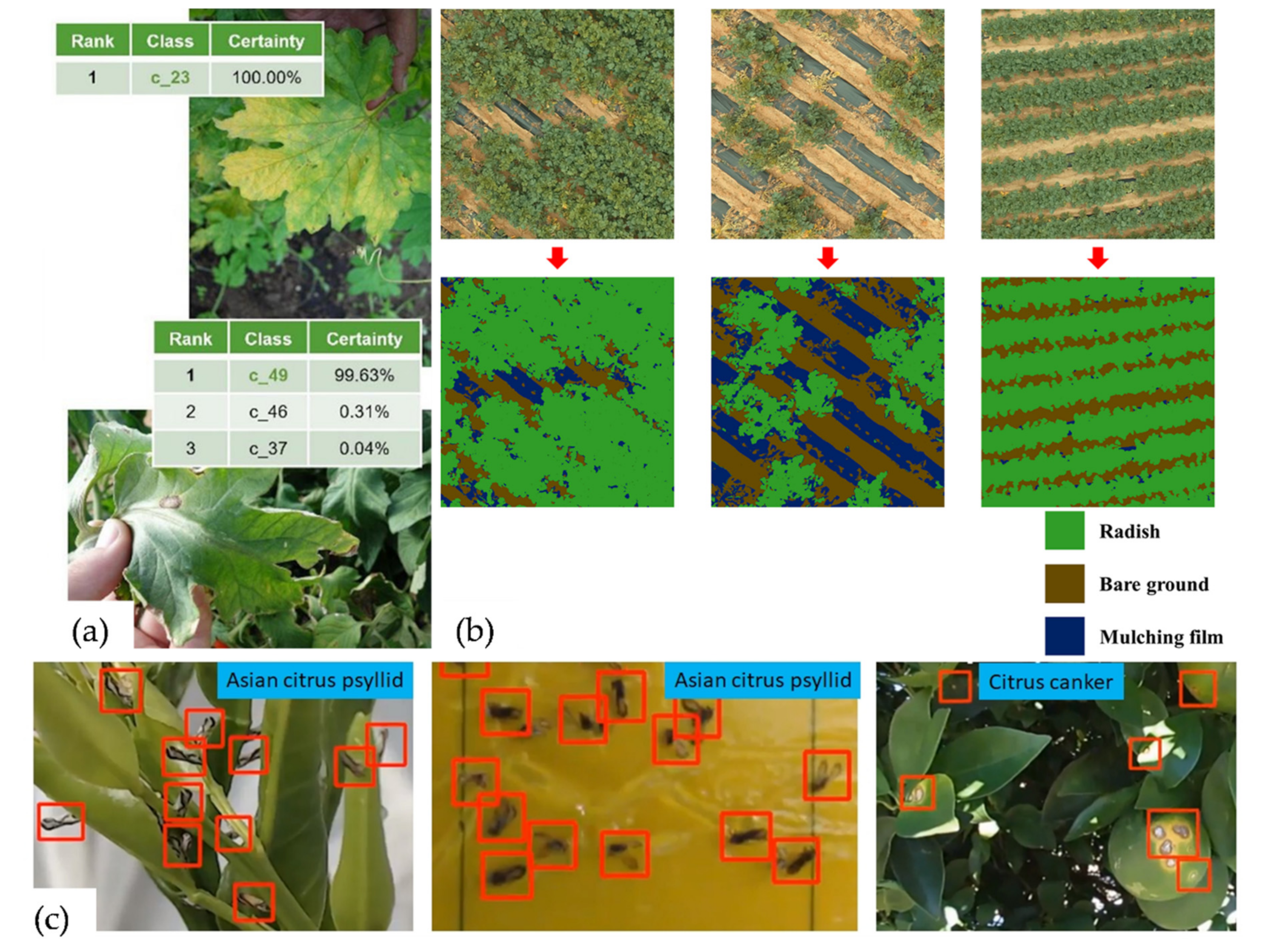
Applications of deep learning for crop stress detection based on different image analysis. (a) Classification (images from [47]), (b) segmentation (images from [48]), and (c) object detection (images from [49]).


Table 1.
Applications of deep learning for crop stress classification.
| Reference | Sensor | Stress Type | Method | Application |
|---|---|---|---|---|
| [50] | RGB sensor | Biotic | CNN pre-trained with AlexNet | Apple leaf Diseases |
| [51] | RGB sensor | Biotic | CNN pre-trained with GoogLeNet | Cassava leaf Diseases |
| [52] | RGB sensor | Biotic | FCN pre-trained with VGG, CNN pre-trained with VGG | Wheat leaf diseases |
| [53] | RGB sensor | Biotic | CNN | Maize leaf disease |
| [54] | RGB sensor | Abiotic | DNN | Tomato water stress |
| [55] | RGB sensor | Abiotic and biotic | Faster R-CNN, R-FCN, SSD pre-trained with VGG, ResNet | Nine tomato diseases and pests |
| [56] | RGB sensor | Biotic | CNN pretrained with VGG16 and MSVM | Five major diseases of eggplant |
| [57] | RGB sensor | Abiotic and biotic | CNN | Eight different soybean stresses |
| [58] | Hyperspectral imaging | Biotic | CNN and RNN | Wheat Fusarium head blight disease |
| [59] | RGB sensor (datasets from plantVillage) | Biotic | VGG 16, Inception V4, ResNet, DenseNets | 38 different classes including diseased and healthy images of leaves of 14 plants |
| [60] | RGB sensor | Biotic | SIFT encoding and CNN pretrained with MobileNet | Grapevine esca disease |
| [61] | RGB sensor | Abiotic | DCNN pretrained with ResNet | Maize drought stress |
| [62] | RGB sensor (datasets from plantVillage) | Biotic | CNN pretrained with AlexNet, GoogLeNet, Inception v3, ResNet-50, ResNet-101 and SqueezeNet. | Grapevine yellows disease |
| [63] | RGB sensor | Biotic | CNN | Rice blast disease |
| [64] | RGB sensor (datasets from AI Challenger Global AI Contest) | Biotic | PD2SE-Net based on CNN and ResNet | Apple, cherry, corn, grape, peach, pepper, potato, strawberry, tomato diseases |
| [65] | Smartphones | Biotic | CNN AlexNet, GoogLeNet, ResNet, VGG16, MobileNetV2 | Coffee leaves with rust, brown leaf spot and cercospora leaf spot |
| [66] | Hyperspectral imaging | Biotic | CNN | Yellow rust in winter wheat |
| [67] | RGB sensor | Biotic | CNN | 14 crop species with 38 classes of diseases. |
| [68] | Hyperspectral imaging | Biotic | GAN | Tomato spotted wilt virus |
| [69] | RGB sensor | Biotic | GAN, VGG16 | Tea red scab, tea red leaf spot and tea leaf blight |
Note: SIFT: Scale-invariant feature transform.
Table 2.
Applications of deep learning for crop stress segmentation.
| Reference | Sensor | Stress Type | Method | Application |
|---|---|---|---|---|
| [75] | Smart phone | Biotic | CNN | Cucumber diseases |
| [76] | RGB (from Plant Village, datasets) | Biotic | Fractal Texture Analysis (SFTA) and local binary patterns (LBP) combined with VGG16 and Caffe-AlexNet | Fruit crops diseases |
| [77] | RGB sensor | Biotic | Mask R-CNN | Rice leaf diseases |
| [78] | RGB sensor (from AI Challenger 2019) | Biotic | CNN pre-trained with U-Net | Nineteen plant diseases |
| [79] | RGB sensor | Biotic | Global pooling dilated convolutional neural network (GPDCNN) | Cucumber leaf disease |
Table 3.
Application of deep learning for crop stress object detection.
| Reference | Sensor | Stress Type | Method | Application |
|---|---|---|---|---|
| [55] | RGB sensor | Abiotic and biotic | Faster R-CNN, R-FCN | Nine tomato diseases and pests |
| [60] | RGB sensor | Biotic | CNN pretrained with RetinaNet | Grapevine esca disease |
| [82] | RGB sensor | Biotic | YOLOv2 and YOLOv3 | Mosquito bugs and red spider mites |
| [83] | RGB sensor | Biotic | Mask R-CNN | Northern leaf blight of maize |
| [86] | Smartphone | Biotic | Faster R-CNN | Rice false smut |
| [87] | RGB image from the Internet | Biotic | Faster R-CNN and Mask R-CNN | Ten tomato disease |
| [88] | Smartphones | Biotic | Faster R-CNN | Strawberry verticillium wilt |
| [89] | RGB image | Biotic | Faster R-CNN | Sweet Pepper Disease and Pest |
© 2020 by the authors. Licensee MDPI, Basel, Switzerland. This article is an open access article distributed under the terms and conditions of the Creative Commons Attribution (CC BY) license (http://creativecommons.org/licenses/by/4.0/).
Share and Cite
MDPI and ACS Style
Gao, Z.; Luo, Z.; Zhang, W.; Lv, Z.; Xu, Y. Deep Learning Application in Plant Stress Imaging: A Review. AgriEngineering 2020, 2, 430-446. https://0-doi-org.brum.beds.ac.uk/10.3390/agriengineering2030029
AMA Style
Gao Z, Luo Z, Zhang W, Lv Z, Xu Y. Deep Learning Application in Plant Stress Imaging: A Review. AgriEngineering. 2020; 2(3):430-446. https://0-doi-org.brum.beds.ac.uk/10.3390/agriengineering2030029
Chicago/Turabian StyleGao, Zongmei, Zhongwei Luo, Wen Zhang, Zhenzhen Lv, and Yanlei Xu. 2020. "Deep Learning Application in Plant Stress Imaging: A Review" AgriEngineering 2, no. 3: 430-446. https://0-doi-org.brum.beds.ac.uk/10.3390/agriengineering2030029