A Deep Learning Approach for Weed Detection in Lettuce Crops Using Multispectral Images

Abstract

Weed management is one of the most important aspects of crop productivity; knowing the amount and the locations of weeds has been a problem that experts have faced for several decades. This paper presents three methods for weed estimation based on deep learning image processing in lettuce crops, and we compared them to visual estimations by experts. One method is based on support vector machines (SVM) using histograms of oriented gradients (HOG) as feature descriptor. The second method was based in YOLOV3 (you only look once V3), taking advantage of its robust architecture for object detection, and the third one was based on Mask R-CNN (region based convolutional neural network) in order to get an instance segmentation for each individual. These methods were complemented with a NDVI index (normalized difference vegetation index) as a background subtractor for removing non photosynthetic objects. According to chosen metrics, the machine and deep learning methods had F1-scores of 88%, 94%, and 94% respectively, regarding to crop detection. Subsequently, detected crops were turned into a binary mask and mixed with the NDVI background subtractor in order to detect weed in an indirect way. Once the weed image was obtained, the coverage percentage of weed was calculated by classical image processing methods. Finally, these performances were compared with the estimations of a set from weed experts through a Bland–Altman plot, intraclass correlation coefficients (ICCs) and Dunn’s test to obtain statistical measurements between every estimation (machine-human); we found that these methods improve accuracy on weed coverage estimation and minimize subjectivity in human-estimated data.

1. Introduction

As the world population increases, so does the demand for food. Taking into account that land, water, and labor are limited resources, it is estimated that the efficiency of agricultural productivity will increase by 25% by the year 2050 [1]. Therefore, it is crucial to focus on the problems faced by the agricultural industry. Liakos et al. [2] propose different categories to classify the challenges faced by machine learning in precision agriculture, such as livestock management, water management, soil management, detection of plant diseases, crop quality, species recognition, and weed detection. New developments in this last category would help to face the most important biological threat in crop productivity. According to Wang [3], an average of 34% of production is lost because weeds directly compete for nutrients, water, and sunlight. Furthermore, weeds are harder to detect due to their non-uniform presence and their overlap with other crops.

The oldest technique used to control weeds in crops is manual weeding. However, it is labor- and time-consuming, which makes it inefficient for larger scale crops. Today, agricultural industry has chemical weeding systems, and to a lesser extent, mechanic weeding systems, but in our context (Andean Highlands), 75% of the vegetables produced, such as lettuces, have manual weeding, which makes production even more inefficient and expensive [4]. Moreover, there is a very high margin of error regarding weeding and these systems may end up damaging the plants [2].

Authors should discuss the results and how they can be interpreted from the perspectives of previous studies and the working hypotheses. The findings and their implications should be discussed in the broadest context possible. Future research directions may also be highlighted.

Due to the herbicide usage policies in some countries and the high cost in areas with underdeveloped agricultural processes, there is a need to carry out weed detection and calculation processes in order to reduce the environmental impact of herbicides and optimize their use [5].

However, regardless of the control method, field information will always be needed to make decisions. This has been done through conventional sampling, which consists of visually estimating the percentage of weeds with respect to the soil (coverage), the number of individuals by area (density), the number of times that each species appears in a certain number of samplings (frequency), or the estimation of weed weight by area (biomass) [6].

The methodologies of conventional sampling widely vary depending on the objective of the information required. There are variations regarding the number of sampling sites, their distribution in the field, and the variables used, among other things. Ambrosio et al. [7] affirms that conventional sampling by square grids is one of the simplest and most effective methods, since weeds have an aggregate distribution and weed density can be determined as a variable that can follow a Poisson distribution or a negative binomial probability distribution [8].

According to López Granados et al. [9] the main purpose of SSWM (site-specific weed management) systems is to spray herbicides on groups of weeds, taking into account their density and the type of weed. In early growth stages, crops are highly vulnerable so it is important to have the information to support management decisions and efficiently control weeds. Additionally, in our context, in a plot there could be 20 or more different species of weeds in a one-hectare field, reaching 100% coverage in 1–2 months, with some of the weeds seeding in 1–2 months and having four to five cohorts of weeds in a 4–6 month crop production cycle [10]. This could happen in any month of the year, since we do not have temperate climate seasons (only wet and not so wet seasons).

However, their detection might be difficult because the crop plants are small and may have some characteristics similar to those of weeds. Therefore, satellite images do not provide the necessary information. Unmanned aircraft systems (UASs) offer a better solution, since they can be automatically or remotely controlled at short and long distances, capturing digital images at the height and frequency required by the user, which varies depending on the type of UAV (unmanned aerial vehicle) that operates the system [11,12].

Additionally, these UAVs can be equipped with multispectral cameras that offer more information than an RGB digital image, since they capture spectral bands not recognized by the human eye—such as near infrared (NIR)—providing information on aspects such as the reflectance of visible light and vegetation indices. These components allow one to find important correlations that help with making different estimates.

Multispectral sensors also offer other benefits such as facilitating the differentiation of some types of plants from their environment, thanks to the different vegetation indices such as the chlorophyll absorption index and the cellulose absorption index, among others. Moreover, they provide more information during the feature extraction processes, such as those used in the OBIA methods (object-based image analysis) [11,13,14,15,16], and SVM-based (vector support machines) classification techniques [8,17,18].

Multispectral images depend on the climatic conditions of the days in which they are captured, since climate changes a plant’s reflectance due to the difference in the amount of light absorbed. Additionally, in the early stages of some crops, certain vegetation indices are similar to those of weeds that surround them; that fact and cropping systems with mulch soil cover pose some challenges for the classification algorithms, since they do the identification on images that are very complex. These and other challenges were faced using artificial neural networks (ANN), which in the last four years have been the most widely used method of weed detection, as Behmann et al. mentioned in their research on weed detection using images [19,20,21,22,23,24,25,26].

The convolutional neural networks (CNN) are setting a strong trend for the classification and identification of image-based patterns. Among the articles reviewed are some of the convolutional neural network architectures that are well-accepted for weed identification, such as AlexNet, ResNet, RCNN, VGG, GoogleNet, and FCN (fully convolutional network) [27,28,29,30,31,32,33,34,35,36,37,38]. The main advantage of such methods is that they speed up the manual labeling of data sets, while maintaining a good classification performance. This approach stands out among the other conventional index-based approaches (such as NDVI) because it is 98.7% accurate. Additionally, since images are the input itself, the problems of SVM and ANN regarding the selection and extraction of features are reduced. Therefore, it represents a major trend in terms of machine learning and pattern recognition, in addition to its great performance with all types of images; so CNNs are increasingly used for weed detection [38,39].

Previous works in lettuce fields such as those of Raja et al. [40] and Elstone et al. Raja et al. [41] obtained good results for weed and crop identification using RGB and multiespectral images, but weeds in highland tropical conditions have different forms and grow in big patches, making detection difficult; therefore, we developed methods to firstly perform vegetation detection, secondly perform crop detection, and lastly identify and quantify weeds in the field.

This study compared the weed quantification results of three methods which used machine learning and multispectral images to the results of three experts in agronomy-weed management with different weed estimation levels of training in the same set of images. The first one was based on histograms of oriented gradients and support vector machines (method 1: HOG-SVM); the second one used a CNN (convolutional neural network) that specializes in object detection (method 2: YOLO); and the third one used masks for edge detection and the "regions with CNN features" algorithm for crop recognition. The main objective in this study was to implement and establish a comparison between one machine learning method and two deep learning approaches for weed detection. Additionally, we wanted to compare those results with three different estimations of weed science experts. Notice that each expert had a different level of academic background and the subjectivity component in every estimation could establish significant differences in statistical terms.

2. Materials and Methods

The images and the methods used are described below, along with their most important elements. Then, the performances of these weed quantification methods are described, and finally they are compared against the estimates of three weed experts.

2.1. Dataset

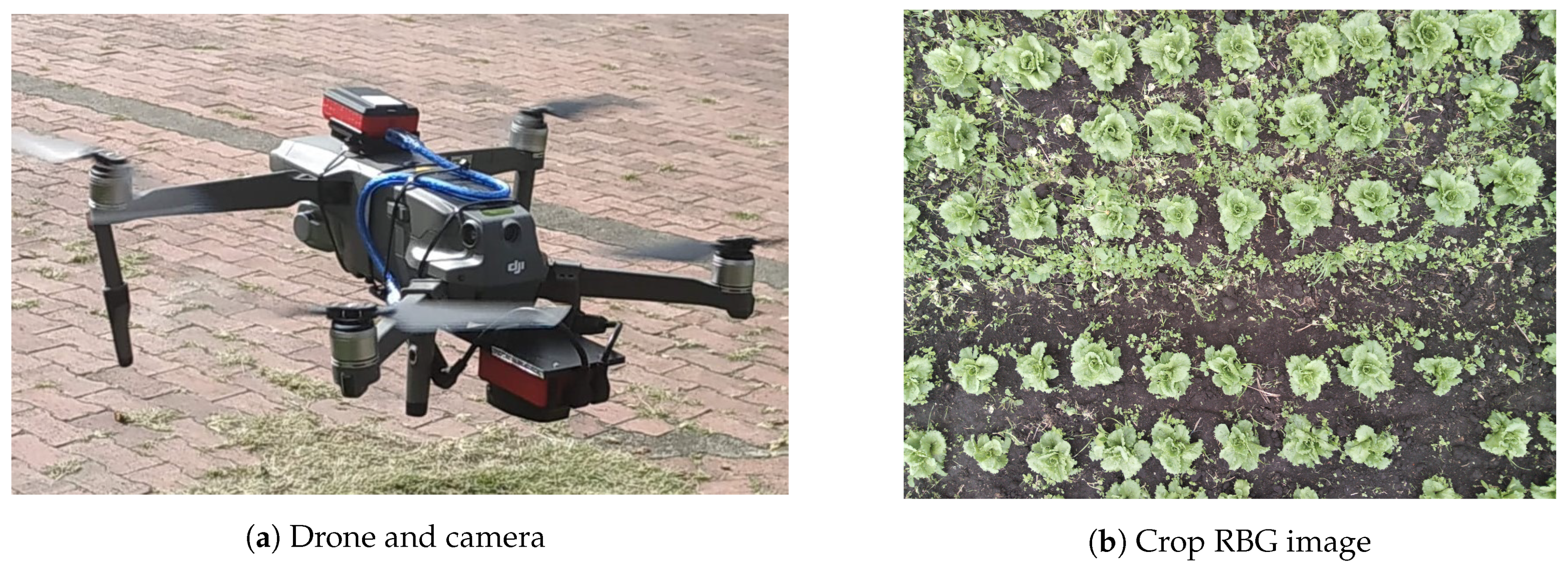
The drone used was a Mavic Pro with the Parrot Sequoia multispectral camera (Figure 1a), which followed an automatic flight plan at 1 m/s and 2 m high. Regarding the weather conditions, the flight was made around 15 h, partly cloudy but with good sun exposure. The total route of the 100 images used corresponds to approximately 600 m${}^2$.

The photographs were captured in a commercial lettuce crop, 60 days after seeding and 20 days after the first manual weeding. An unmanned aerial vehicle was used to capture images at 2 m height. Later, 100 images were selected, each with a pixel size of 1280 × 960 (0.22 cm/px) and four spectral bands: green 550 nm, red 660 nm, red edge 735 nm, and near infrared 790 nm. Finally, a false green image was generated, which is the union of the red, green, and near infrared bands, in order to highlight the vegetation (Figure 2).

2.2. Experts’ Evaluations

Three experts in agronomy-weed management made visual estimations pf weed coverage for 100 images with 2219 lettuces and high, medium, and low levels of weeds. It is noteworthy that the experts had different training levels in weed estimation: expert 1 had a BSc in agronomy with some weed coverage estimation training, expert 2 had an MSc in agronomy with proper training, and expert 3 had a PhD in weed science and extensive experience in estimation of coverage of weeds.

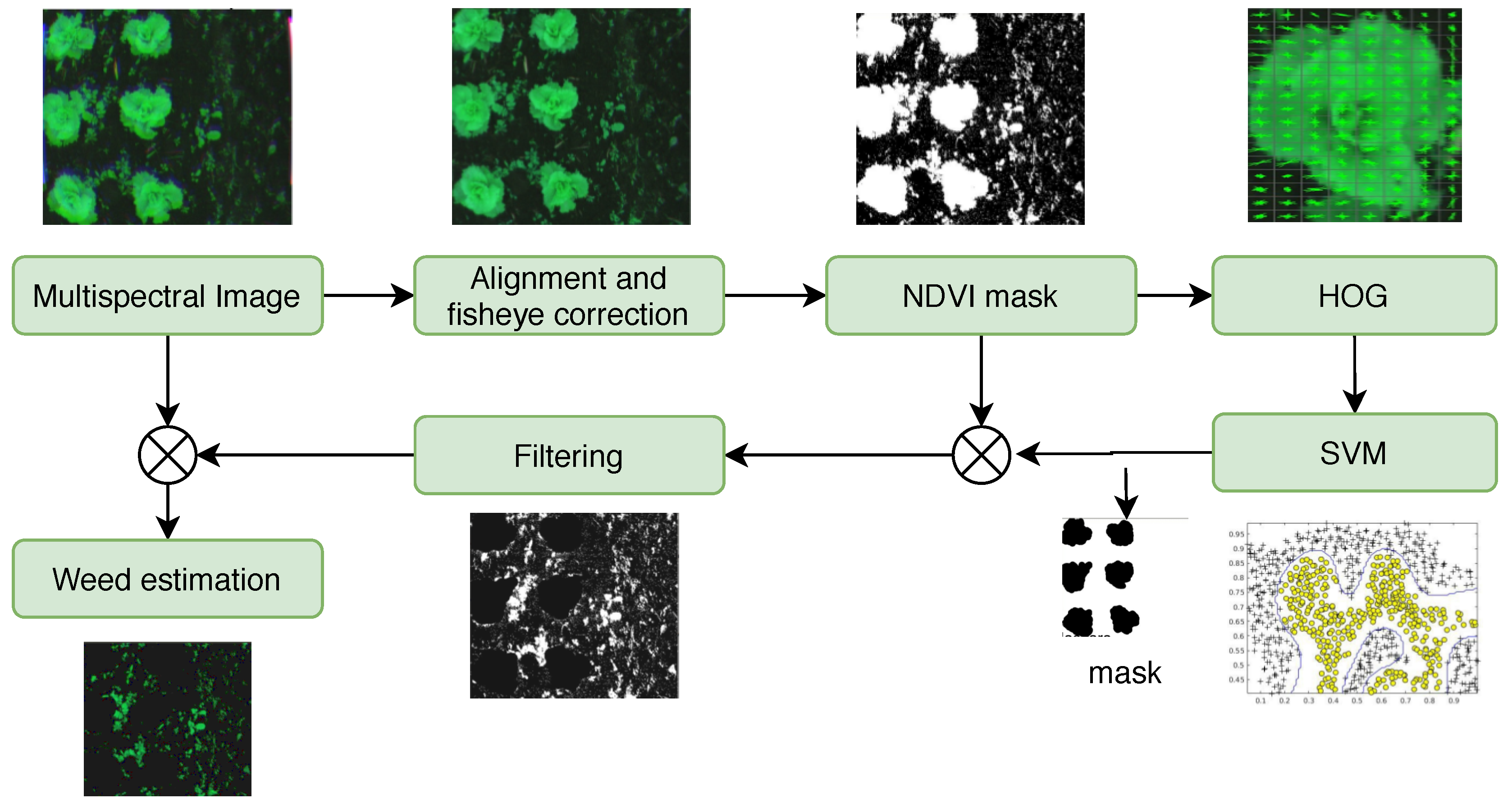
2.3. Method 1: HOG-SVM

Support vector machines are mathematical models whose main objective is to find the optimal separating hyperplane between two different classes. This paradigm is based on a type of vectors known as support vectors that can be in a space of infinite dimensions mapped by a kernel and a cost parameter [42]. In this case, the histograms of oriented gradients (HOG) were used as the technique to extract the features in each image object. Subsequently, a training process was carried out using the polynomial kernel with the best performance in [8], using 1400 images. The main objective of this method is to identify the class (weed or lettuce) of a specific object using a mask created through the NDVI and the OTSU method; the Figure 3 shows the flow diagram.

A histogram of oriented gradients represents an object based on the magnitude and orientation of the gradient from a specific set of pixel blocks [8]. This type of feature allows obtaining the shape of a plant with a well-defined geometry. Figure 3 shows the detection process, including the preprocessing phase using the NDVI index as a background estimator. This index creates a mask that removes some objects such as the ground and elements that are not related to vegetation. On the other hand, the edges of this mask are calculated and their respective coordinates are transferred to the original image, thereby providing objects with photosynthetic activity. The features are extracted from these objects using histograms of oriented gradients, which in turn serve as input to a pre-trained support vector machine. The SVM determines whether the detected objects belong to the lettuce class. The objects belonging to that class are stored in a new mask called crop mask (see Figure 3).

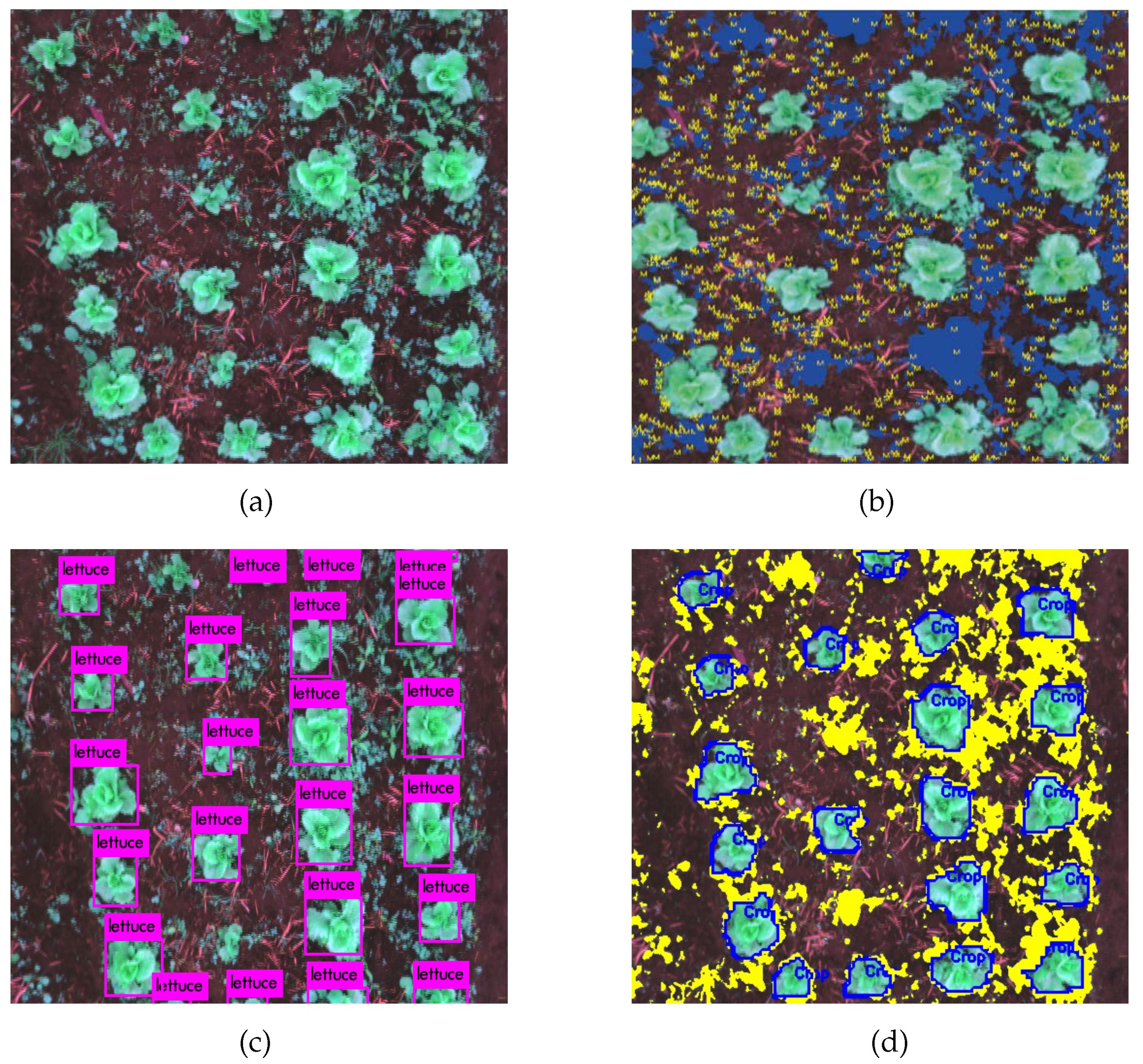
Then, this mask is multiplied by the mask obtained through the NDVI index, eliminating all the lettuce objects from the image and leaving only the objects with photosynthetic activity that generally belong to the weed class. Finally, the percentage of white pixels with respect to the total area of the image is calculated in this new weed mask, in order to determine weed coverage as shown in Figure 4b.

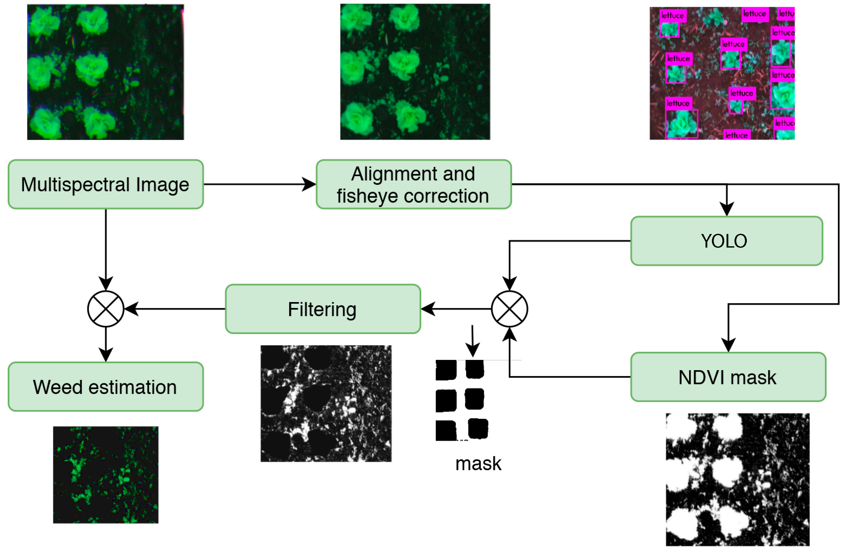
2.4. Method 2: CNN-YOLOv3

YOLO (you look only once), as its name implies, is a neural network capable of detecting the bounding boxes of objects in an image and the probability that they belong to a class in a single step. YOLO uses convolutional networks and it was selected for its good performance in object and pattern recognition, which has given it a recent good reputation in fields such as the recognition of means of transportation and animals, and the tracking of moving objects. The first version of YOLO came out in 2016 [43]; its architecture consisted of 24 convolutional layers working as feature extractors and two dense or fully connected layers that performed predictions. YOLOv3 was used for its significant enhancements and feature extraction layers which were replaced by the Darknet-53 architecture [44].

As seen in Figure 5, once the model is trained to identify the crop (Figure 4c), an algorithm uses bounding box coordinates from the model to remove crop samples from the image. Later, a green filter binarizes the image, so pixels without vegetation become black, while the pixels accepted by the green filter become white. Finally, vegetation that does not correspond to the crop is highlighted, thereby simplifying the percentage calculation of weeds per image.

In order to get the most out of YOLO in terms of effective detection of objects and speed, it was decided not to use edge detection and to consider the entire bounding box generated by the model as crops, although this might affect weed calculation since the closest weed to the crop could be lost during estimation.

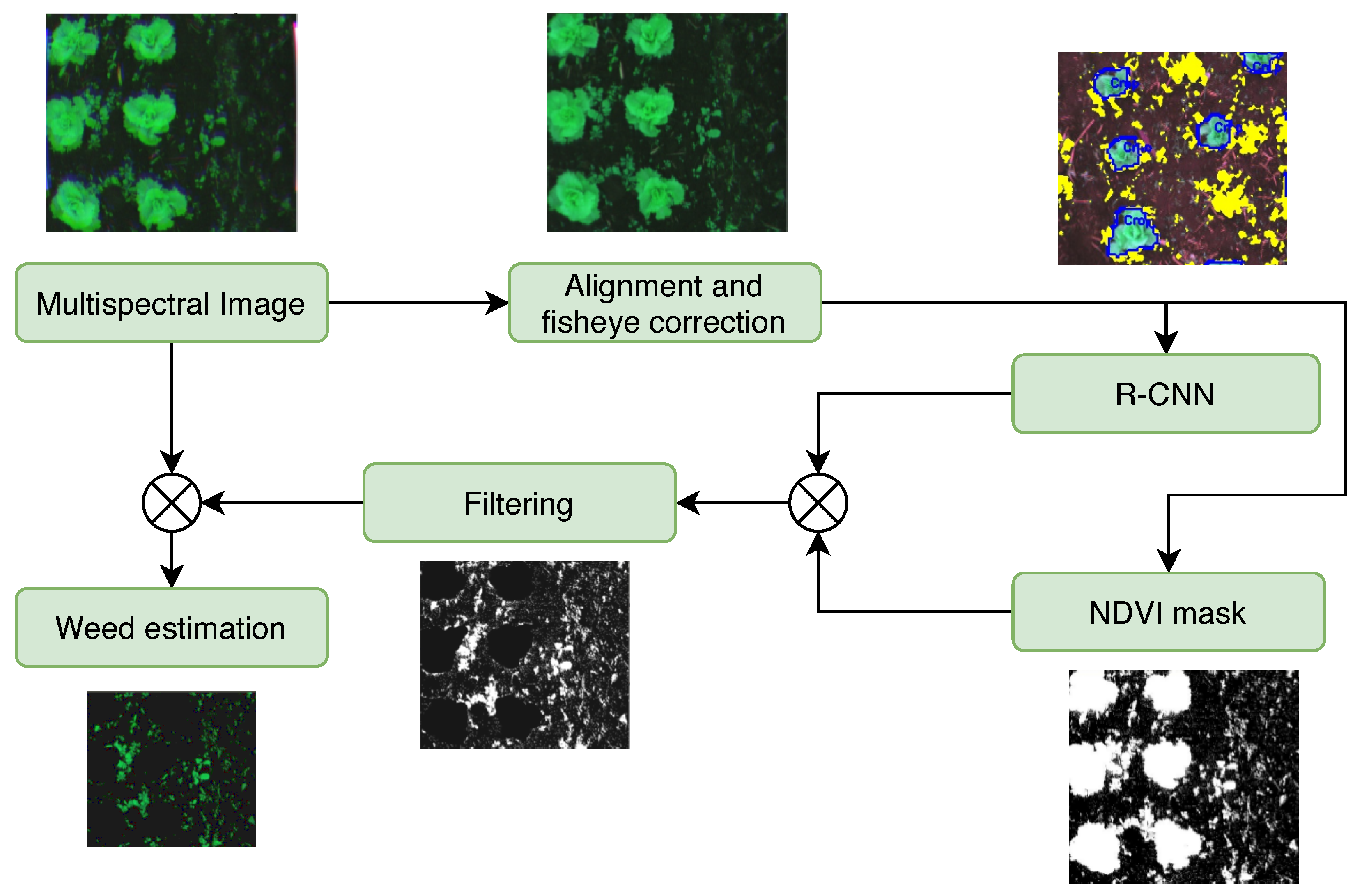
2.5. Method 3: Mask R-CNN

RCNN uses the “selective search for object recognition” algorithm [45] to extract 2000 regions from the image. They feed a convolutional neural network—in this case Inception V2—which extracts features that will be introduced to an SVM in order to classify the object in corresponding class. Additionally, when using masks in the training process of this method, an instance segmentation [46] is obtained, which provides detailed information about pixels that belong to the class. The training method used in this phase involves labeling crops as a “bounding box” and labeling masks related to each class. This mask comes from the closed region corresponding to crop that is inside corresponding “bounding box”. The architecture used [46] allows one to associate pre-trained masks with detected instances. These masks allow for obtaining the edges of an object without having to calculate them, as in case of the SVM-HOG method.

Unlike SVM-HOG, weeds are estimated by initially processing the complete image with a convolutional network. This network delivers corresponding crop masks in a binary image (Figure 4d). Furthermore, the NDVI index allows one to eliminate background image, leaving only objects corresponding to weeds and lettuce (Figure 6). Finally, this image is mixed with masks generated by neural network to obtain the image of weeds; the percentage of weeds in the image is calculated with respect to the total area.

2.6. Experimental Setup

For this study, three models of each method were trained with 913 samples labeled manually by experts. In the training process, a machine with an 8-core Xeon processor, 16 GB of RAM, and a GTX 1060 6 GB graphic card was used. Training metrics included accuracy, specificity, and precision, among others.

In the performance evaluation and comparison, the best model of each method was selected by taking into account their confusion matrices, coverage values, and evaluation times. Later, they were implemented in separate environments with the same characteristics: 4-core Xeon processor and 8 GB of RAM, without the graphics card. Regarding programming languages, method 1 used C++, method 2 used the Darknet framework for training and Python for evaluation, and method 3 used Python with TensorFlow library.

2.7. Performance of Methods

Several models were trained; we reduced number of training images to leave the maximum possible number of images for validation and comparison with experts (58 images with 1306 lettuces), with a limit of 85% of F1-score for the three methods. In total for training of the final models, 42 images were used, which contained 913 lettuces, approximately 41% of total samples.

Table 1. The performance evaluation of ML models in testing phase.

Metrics	Model
	HOG-SVM	YOLO	R-CNN
Accuracy	79%	89%	89%
Sensitivity	83%	98%	91%
Specificity	0%	0%	0%
Precision	95%	91%	98%
F1-Score	88%	94%	94%

shows metrics obtained by each model for crop detection calculated using confusion matrices of each method; the three models performed well. However, in this case, accuracy does not provide enough information, since this model was evaluated using a single class and without negative samples, as evidenced by the results of specificity. In terms of sensitivity and precision, models that used YOLO and R-CNN stand out. Their high scores indicate that crop estimation was very accurate for these models without detracting from performance of HOG-SVM model. This is well summarized in the F1-scores of the three models.

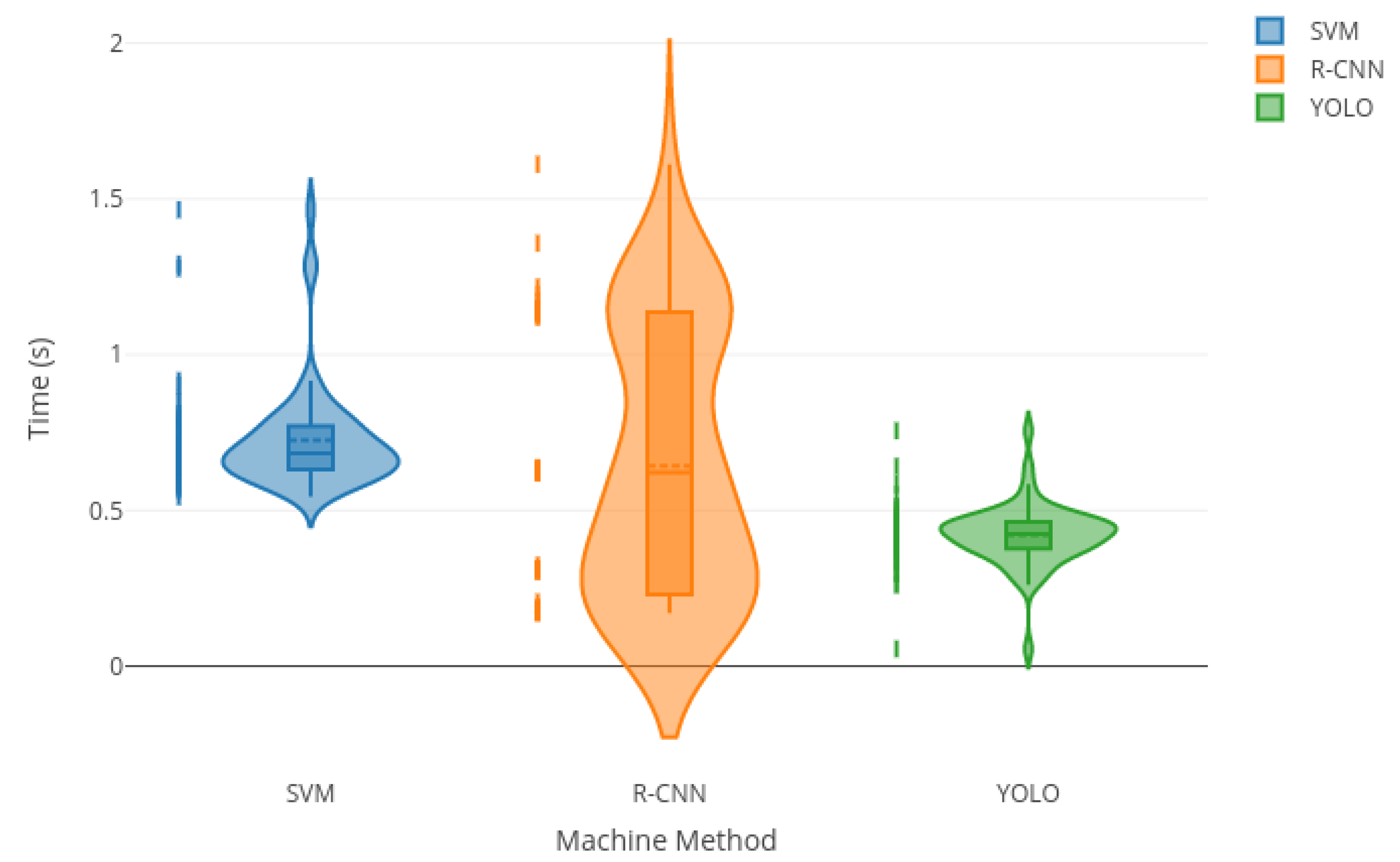
To compare the time spent by each technique, several of the non-parametric methods used were reviewed (Nemenyi, Wilcox, Kruskal, Dunn). Due to the lack of normality, Wilcox was chosen, since data corresponded to dependent samples; in fact, they were the same population. There were statistical differences in the time used by different methods. In the boxplot,Figure 7, it can be seen that HOG-SVM and YOLO are more consistent in terms of time, while time is more variable in RCNN.

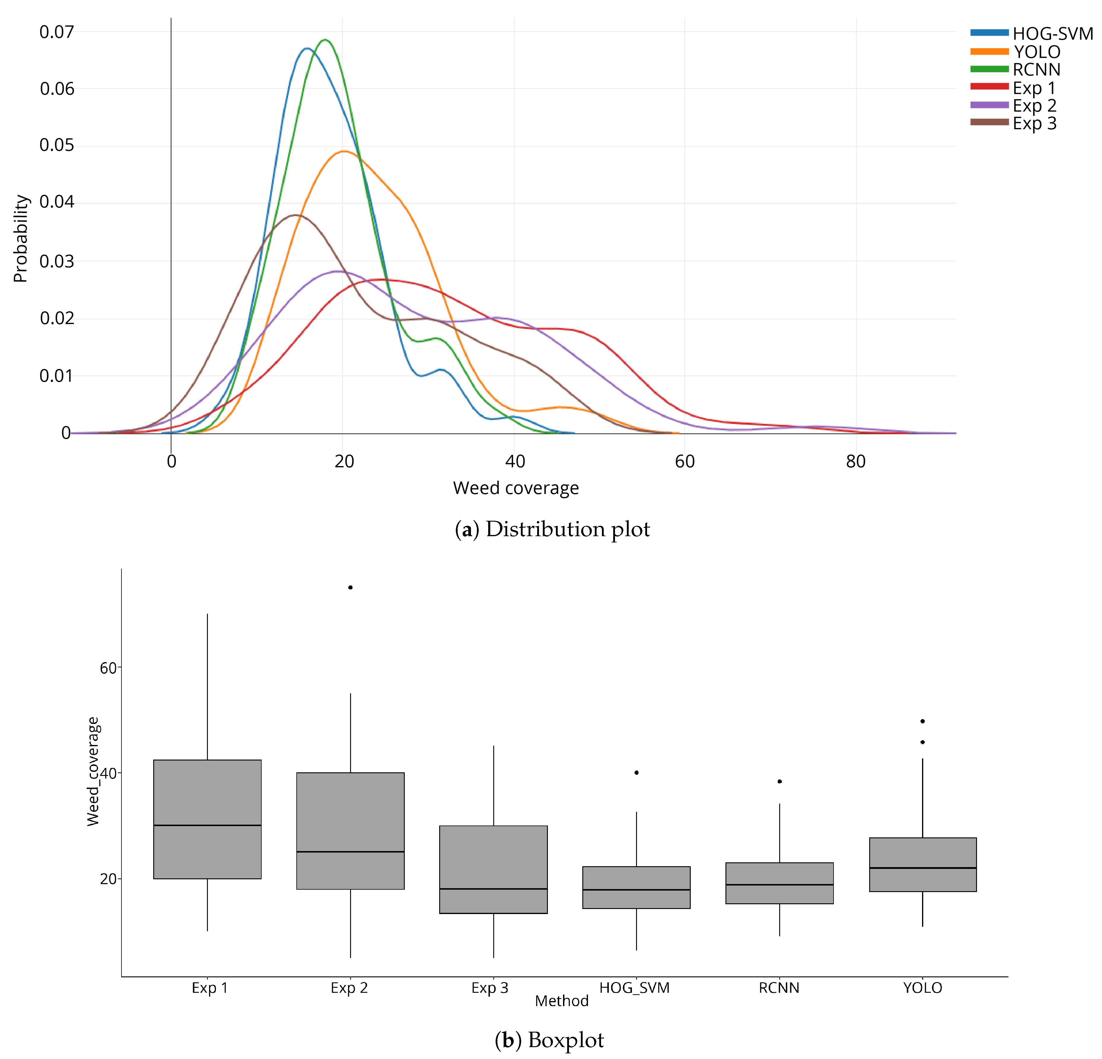
According to Ambrosio [7], the samples with square grids suggest that the variable of weed density follows a negative binomial probability distribution, a distribution similar to those presented in Figure 8a, which indicates that both estimates (models and experts) behaved as expected. However, curves can be classified into three groups: First, models that used HOG-SVM and RCNN, which had similar and homogeneous distributions with respect to others. The second group includes the third expert and model trained with YOLO; their behavior suggests their estimates have a similar trend. Finally, the third group includes the first and second experts, whose distributions were similar, but very different in comparison to the others. This suggests that their data tended to overestimate the high coverage of weeds compared to the others, which proves that subjectivity is one of the main problems in human estimation of weeds. Opposite results where found in Andujar et al., as they found that visual estimations bias is to underestimate high-coverage weeds [47].

3. Results and Discussion

Regarding the coverage value, a boxplot was developed (Figure 8b), in order to explore possible differences. Then, the Dunn’s test (

Table 2. Dunn test matrix with the different p-values between methods and experts.

	RCNN	Exp1	Exp2	Exp3	HOG-SVM
Exp1	8.7 × 10${}^{-7}$	-	-	-	-
Exp2	0.00430	0.45020	-	-	-
Exp3	0.99370	1.7 × 10${}^{-5}$	0.02827	-	-
HOG-SVM	0.99405	3.5 × 10${}^{-8}$	0.00048	0.87911	-
YOLO	0.25900	0.01379	0.69951	0.59922	0.07420

) was performed to verify the existence of significant differences. Intraclass correlation coefficients (ICC

Table 3. Comparison using ICC (intraclass correlation coefficient) methods and experts.

Methods	ICC	p-Value
RCNN vs. YOLO	0.572	7.76 × 10${}^{-7}$
RCNN vs. HOG-SVM	0.919	9.72 × 10${}^{-26}$
RCNN vs. Exp1	0.112	0.197
RCNN vs. Exp2	0.373	0.00158
RCNN vs. Exp3	0.694	2.99 × 10${}^{-10}$

) were obtained to verify agreement, and finally [47], exploratory analysis was done to compare the correlations and agreement of methods using a correlation matrix and Bland–Altman plots.

Figure 8b shows that RCNN and HOG-SVM are almost identical; YOLO differs a little and is more similar to experts 1 and 2. Conversely, expert 3 is similar to RCNN and HOG-SVM but has more scattered data. Experts 1 and 2 have a higher dispersion since they overestimated the largest coverage values, as illustrated in the Bland–Altman plots.

Table 2 shows that the RCNN and HOG-SVM methods do not have significant differences with respect to YOLO method, nor with respect to expert 3. As for the YOLO method, it only differs from expert 1; expert 1 is different from all methods and experts. On the other hand, expert 2 is different from all except the YOLO method. Finally, expert 3 is statistically different from the other two experts, but not from any computational method.

Those variations were due to the differences in education and training, since the expert 1 was an agronomy professional, but with little training in the quantification of weeds. Expert 2 was an agronomy professional with training in the quantification of weeds. Expert 3 was a highly trained agronomy doctor. This was corroborated later with the ICC (intraclass correlation coefficient).

The correlation matrix (Figure 8c) shows that method 2 (YOLO)—among the computational techniques—and expert 1—among the experts—were the most inconsistent. However, comparing different evaluation methods is a complex task, since usually there is no standard or true value. Thus, one of the most used, but also the most criticized methods is the Pearson correlation. It evaluates the linear association between measurements (variables), but does not evaluate their agreement. Therefore, two methods can have a good correlation but not agreement, or vice versa [48].

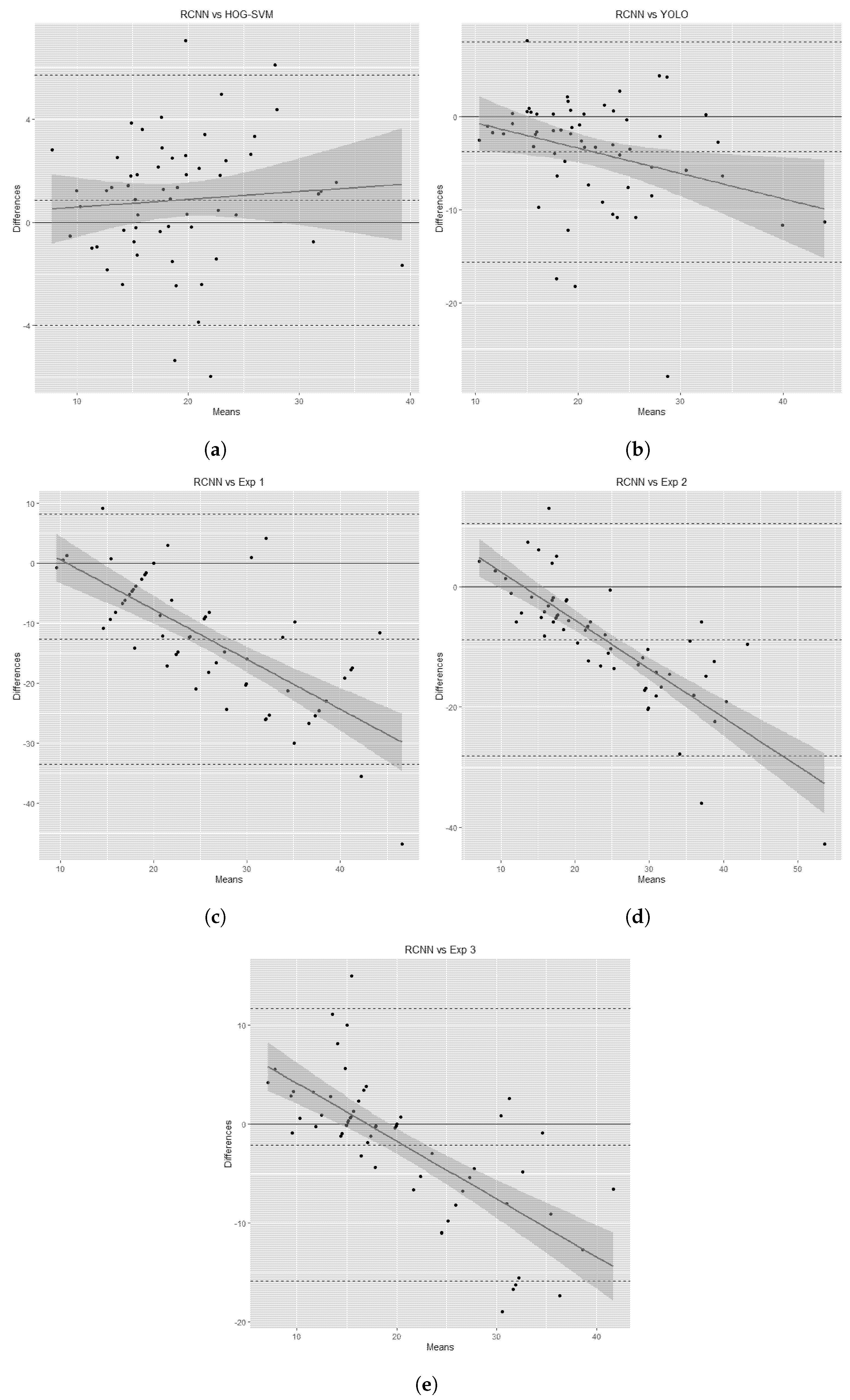
3.1. Analysis and Results Using the Bland–Altman Method

The Bland–Altman graphical method allows one to compare two measurement techniques while taking into account the same quantitative variable, in order to determine agreement limits, biases, and variability. To perform the analysis based on the Blant-Alman method, the R-CNN method and SVM (Figure 9a) were compared. The y axis represents differences in the coverage values for each method, while the x axis represents their mean values.

There are three dotted lines in the Bland–Altman plots. The one in the middle quantifies the mean difference between both methods. The other two represent upper and lower limits of agreement which establish range of differences between one method and the other. The smaller this range is between these limits, the better agreement between methods; a difference more than 10–15 could be unacceptable, since the most common scales for weed management decision support systems are ordinal and its ranks are higher than these values [47]. In Figure 9a, the limits of agreement are between −4 and +5 (dashed lines). As for the blue line, it indicates the regression calculated for the differences, which shows a non-constant systematic bias. In the case of Figure 9a, it has a small positive trend but tended to remain parallel to the x axis. This shows that there is no variability bias, i.e., the data do not scatter more as values of coverage increase. In conclusion, either method can replace the other [49].

When comparing method 3 (RCNN) with method 2 (YOLO based), as coverage increases, YOLO overestimates weed coverage (Figure 9b). The limits of agreement are wider (−15 to +10, dashed lines), and as coverage increases, so does the differences’ variability.

By comparing the most consistent computational method (RCNN) against values obtained by the experts (Figure 9c), it is possible to corroborate the existence of human bias; i.e., high values of coverage are overestimated, in this case up to 32 coverage units. Additionally, limits of agreement increased from −32 to 9 (dashed lines). The average of the expert 1’s data is greater than the average of method 3 by 12 coverage units. Furthermore, it can be seen that experts rounded to integers or multiples of 5 or 10, while the computational methods gave continuous variables.

Expert 1 was not accurate, since for several images, with the same coverage value, the estimate increased or decreased the coverage value by ±10 (Figure 9c). Expert 2 was more accurate because the data for the same coverage value had a difference of ±5 compared to RCNN method. Limits of agreement were slightly lower, from −28 to +8 (dashed lines). However, they were also biased in overestimating the high coverage values (Figure 9d).

For expert 3, limits of agreement were lower, from −16 to +12 (dashed lines, Figure 9c). There was also an overestimation bias but to a lesser extent. However, the low coverage values were also underestimated. Finally, there was no variability bias and average value of the coverage was very close to the average of method 3.

3.2. A Comparison with Previously Published Results

Regarding other authors, there are a few works related to weed detection in lettuce crops; however, most of them are focused on detection with herbicide application purposes via robotics. For example, Raja et al. [40] proposed a weed detection system in lettuce crops using image processing with illumination control incorporated with an RGB camera. Additionally, this system uses a simple thresholding technique in order to detect weeds with an accuracy of 98.1%. This technique is often limited because it depends on light control and as consequence increases the cost of the system. On the other hand, different machine approaches exposed in this paper are able to be invariant to abrupt changes in illumination due to the transfer learning feature of deep learning systems. Thus, in this case, collecting data from environments with changes in their illumination and by re-training the model could be a solution to this problem.

Otherwise, Elstone et al. [41], has her own approach of using a robotic system for detecting lettuces trough a multispectral camera and illumination control system. This approach focuses on NIR reflectivity pixels values and a size classificator assuming that crops will be always larger than weeds. In this case, this assumption could get to many false positives in each detection. This approached achieved 88% accuracy.

Table 4. Comparison between lettuce detection methods.

Approach	Accuracy	F1-Score	Light Sensitive	UAV	Rover	Camera	Size Sensitive
Thresholding [40]	98.1%	N/A	YES	NO	YES	RGB	NO
Size and reflectivity [41]	88%	N/A	YES	NO	YES	MULTI	YES
SVM	79%	88%	NO	YES	NO	MULTI	NO
YOLO	89%	94%	NO	YES	NO	MULTI	NO
R-CNN	89%	94%	NO	YES	NO	MULTI	NO

presents a comparison between the methods that were mentioned and the approaches presented here.

Another important remark about the comparison established in Table 4 is related with the use of deep learning models for weed detection instead of classical image processing techniques reflected in [40,41]. This is because deep learning models have great generalization capabilities and can be used with different kinds of lettuce crops, no matter the geographical location. In contrast, classical image processing methods are involved in local calibrations for the illumination control system. Additionally, reflectivity values depend drastically on sun conditions and geolocation. Moreover, those techniques definitely will not work with crops with many weeds in an advanced growth stage. Meanwhile, those methods that include convolutional neural networks such as YOLO and Mask R-CNN can get the main features of a lettuce by themselves, even features that are outside of human visual perception, no matter how many weeds are in the picture. This advantage is very useful when the weed is the same size as the lettuce—solving in this way the limitation presented in [41]. Finally, the fact that this approach does not involve the construction of a complex system that needs lighting control and that it works on a drone allows greater flexibility with quite acceptable results regarding its performance as a weed detector. This set of deep learning models can be easily adapted to aerial fumigation systems to perform herbicide application tasks in a faster way and with similar results to those found in previous literature.

4. Conclusions

Weed detection using multispectral imaging continues to be an important task, since weed control is of vital importance for agricultural productivity. Therefore, the development and improvement of current computational methods is essential. Although the process can be difficult due to the lack of consistency and distinctive morphological features to locate weed, there have been significant improvements in terms of accuracy and speed of detection for a specific crop, thereby enabling one to discriminate between weeds and non-weeds.

Comparing the estimation made by the experts and the trained models reveals one of the main problems that must be addressed using machine learning in precision agriculture: the high error related to subjectivity of the expert when estimating weeds. This makes it more difficult to obtain a correct consensus from the experts and extends the error to the calculations of working hours, and quantity and cost of materials, among others. Therefore, this study demonstrates that pre-trained models for weed estimation are a reliable source with less uncertainty that can be adopted by professionals dedicated to weed control.

The good performances of the methods were mainly due to different approaches to address the problem of weed estimation: vegetation identification, crop detection, and weed quantification. In principle, two weed and crop classes were selected, taking positive and negative samples of both classes. The problem was the identification of the weed because it has just a few fixed characteristics, which makes identification difficult. This generated a high error rate, so the vegetation was identified through multispectral bands. In this way, the model focuses on identifying only the crop and thus facilitates calculation of the remaining vegetation—in this case weeds.

The YOLO model is attractive, not only because of its demonstrated speed regarding other deep neural network architectures, but because although the crops were analyzed as rectangles while ignoring the closest weed to the crop, it did not significantly affect estimation regarding evaluation from experts. However, the R-CNN model stood out for its accuracy in locating the crop and showing the edges very precisely, a method that can be recommended to address other problems in the sector, such as fruit identification.

It was demonstrated that the HOG-SVM method performed very well, and considering that it needs less processing capacity, it is a very good option for IoT solutions.

The Bland–Altman method showed that methods based on HOG-SVM and RCNN are the most similar in terms of evaluation; therefore, they are considered the most consistent. In contrast, the YOLO method overestimates the high values of weed coverage when compared to the other two. Now, although the human bias of rounding values made the experts less precise, when comparing them with methods 1 and 3, it was clear that there was overestimation and underestimation in all three cases, but to different extents. This indicates that the variability in evaluation is linked to the level of experience and is perhaps the most serious problem in human visual estimation. This happens because over-estimating can lead to wrong management decisions. For example, an expert may find the action threshold at experimental level, but a field evaluator will overestimate coverage and this will lead to unnecessary management, increased production costs, and increased contamination.