Definition and Application of a Computational Parameter for the Quantitative Production of Hydroponic Tomatoes Based on Artificial Neural Networks and Digital Image Processing

Abstract

This work presents an alternative method, referred to as Productivity Index or PI, to quantify the production of hydroponic tomatoes using computer vision and neural networks, in contrast to other well-known metrics, such as weight and count. This new method also allows the automation of processes, such as tracking of tomato growth and quality control. To compute the PI, a series of computational processes are conducted to calculate the total pixel area of the displayed tomatoes and obtain a quantitative indicator of hydroponic crop production. Using the PI, it was possible to identify objects belonging to hydroponic tomatoes with an error rate of 1.07%. After the neural networks were trained, the PI was applied to a full crop season of hydroponic tomatoes to show the potential of the PI to monitor the growth and maturation of tomatoes using different dosages of nutrients. With the help of the PI, it was observed that a nutrient dosage diluted with 50% water shows no difference in yield when compared with the use of the same nutrient with no dilution.

1. Introduction

Precision agriculture introduces efficiency to food production, achieving effectiveness that increases along with the technological advances applied to it. With a growing world population, the challenges in food production are increasingly demanding, and many solutions lie in optimizations applied to production techniques. To optimize production, it is necessary to make use of a parameter or indicator value showing the differences between alternative ways of growing an agricultural product and that can determine the most efficient agricultural methods. For example, weight is a widely used production indicator; however, weight does not have discriminatory properties by itself; that is, product quality can be measured by weight but only after carrying out some other filtering methods, such as human observation. To achieve classification capabilities in conjunction with an indicator or quantitative production parameter, it is necessary to resort to computational techniques [1]. In this work, a new general production indicator is introduced, called Productivity Index(PI), which is defined through the digital processing of images taken from cultivation plots and the application of techniques based on neural networks. PI provides a quantitative measure of production and facilitates quality control at the same time. This is done by processing images at the pixel level where discrimination of objects that do not meet certain restrictions takes place. Restrictions are established during the training of a neural network that classifies valid pixels, which are counted to obtain a value that represents the quantitative production of an agricultural plot. In this work, the PI technique is applied to a complete season of a tomato cultivation, and it showed great potential for optimizing crop production.

The application of technology in food production ranges from the use of IoT (Internet of Things) [2] through automatic control based on wireless sensors [3] to cutting-edge artificial intelligence techniques [4]. Currently, among the most popular artificial intelligence techniques is deep learning [5], where a perceptron [6] allows the creation of neural networks that facilitate the classification and identification of patterns. Techniques, such as computer vision [7] and “electronic noses”, have been implemented for the quality control of tomato crops to determine a maturity index for tomatoes [8]. Lin et al. [9] presented a review on computational vision technologies applied to the detection of stress in greenhouse crops. Lin [9] observed that the segmentation or identification of the target continues to be a problem, which is an issue they addressed. The authors of Reference [9] also discussed problems regarding the dosage of water and nutrients in crops, as well as the presence of diseases and pests. Lin et al. [9] then concluded that, to tackle all these problems at the same time, many different algorithms are needed for each crop in order to identify all possible states of the objects of interest.

In this work, a novel algorithm based on neural networks is introduced to address all those problems at the same time. The proposed neural network identifies, at the pixel level, a target and then classifies it according to the training process the network received based on its desired functionality. In this training process, the network learns to effectively identify a target; detect diseases or lack of nutrients and water; and establish a parameter that determines how productive the plot is. Most works in the literature only take consider a certain aspect in food production. The authors of Reference [10] only carried out the preparation and creation of a data set for the training of a neural network. The authors of Reference [11] focused on the complete implementation of the automated acquisition system. The authors of Reference [12] only performed disease detection. Computational vision techniques have been applied to the identification of targets, for example, locating apples in trees using stereoscopic vision [13], detecting tomatoes using the AdaBoost classifier [14], and recognizing groups of tomatoes based on binocular stereo vision [15].

Precision technology and agriculture go together, as is evidenced by the research work carried out in recent years where digital image processing has a high impact. Rezende Silva et al. [16] proposed the use of aerial images of plantations, captured from unmanned aerial vehicles, to monitor the health of crops through methods, such as NDVI (Normalized Difference Vegetation Index), in conjunction with a classification algorithm as a management mechanism for cultivable areas. Image processing was also the main technique used by Treboux and Genoud [17,18], who applied machine learning methods, such as the decision tree ensemble. Kala et al. [19] implemented a SVM (Support Vector Machine) for the detection of plant diseases and optimal application of insecticides. Akila et al. [20] implemented CRFT (Conditional Random Field Temporal Search) to detect plants and monitor their growth. Sudhesh et al. [21] carried out a review on recognition, categorization, and quantification of diseases in various agricultural plants through different computational methods. Yalcin [22] used a deep learning approach to recognize and classify the phenological stages of agricultural plants from their digital images.

In precision agriculture, Convolutional Neural Networks (CNN) are recurring implementations in digital image processing, as can be seen in the works of Umamaheswari et al. [23] and Li et al. [24], where CNNs are used to identify and differentiate weeds from the target crop using a GPU (Graphics Processing Unit) to speed up the process. Furthermore, Yang et al. [25] implemented CNNs to diagnose cold damage to crops through hyperspectral images. Nardari et al. [26] presented a comparison of methods based on CNNs, evaluating the complexity of the model and the performance based on multiple metrics for the task of binary classification of tree segmentation in the environment. In addition, Andrea et al. [27] and Abdullahi et al. [28] used CNNs to identify and classify maize and target plants. The use of other types of neural networks can also be seen in the work by Barrero et al. [29], who implemented weed detection in rice fields with perceptron-based networks. Purwar et al. [30] applied Recurrent Neural Networks (RNN) in satellite images to classify crop plots.

Most of the works in the literature aim to identify an objective and then classify it. This work proposes to go a little further and quantify more precisely what is identified, which is achieved by discriminating pixels by their characteristics. The main idea is that pixels can be discriminated through their RGB (Red, Green, Blue) values with a neural network as a classification instrument. In a technologically advanced hydroponic greenhouse with a controlled environment, it is possible to implement an automatic imaging system for plots and apply digital image processing and artificial intelligence techniques. Furthermore, a production indicator is also proposed in this work, which keeps an automatic record of growth and development of crops and can make comparisons between plots to optimize productive resources and make efficient application and dosing of nutrients.

Koirala et al. [31] presented a survey of deep learning techniques for the detection and counting of objects through digital image processing. They also discussed the weight of the object as a parameter, but they mentioned that only an approximate estimation can be done from the image. The lack of precision for counting objects is especially troublesome when the objects can vary in size, for example, in tomatoes. Five small tomatoes give the same productivity as five large tomatoes if only the count is considered. Clearly, simply counting objects is not a good metric of productivity. On the other hand, if weight is considered instead, there is a control automation problem, i.e., weight does not discriminate by itself the quality of the product. For example, 5 kg of rotten tomatoes would be the same as 5 kg of healthy tomatoes.

Reis et al. [32] presented an identification system for grapes using images. Their main idea is to use the RGB values of pixels to classify objects, which is achieved by defining four main RGB coordinates for a given type of grape and a set of boundaries around those coordinates in order to discriminate if a pixel belongs to the target object or not.

Inspired by the works of Koirala et al. [31] and Reis et al. [32], the main contribution of this work is the definition of a metric called Productivity Index (PI) that uses the images taken from agricultural plots of tomatoes grown with different nutrient dosages to record and monitor their growth. PI is arguably more precise in terms of productivity than a simple counting of objects, and, additionally, it can be used to automate quality control. In contrast to other works in the literature, in this work, a neural network is used for classification and identification of tomatoes. In addition, this work also presents a comparison of production techniques using the PI with data obtained from perceptron-based neural networks.

The rest of this paper is organized as follows. Section 2 presents the techniques used in this work, particularly the architecture of the neural network used, the stages of data processing for the entire proposed system, and the definition of the productivity index. Section 3 presents the results obtained by detailing the numerical values used in the experiments and the experimental environment. Section 4 presents a discussion of the obtained results and compares them against other works in the literature. Finally, Section 5 gives the conclusions of this work.

2. Materials and Methods

To achieve the goal of determining an effective computational indicator of quantitative productivity (the Productivity Index (PI) proposed in this work), it is necessary at some point in the process to discriminate or classify pixels within an image. The focus of this work is on identifying a target fruit or vegetable product by examining the corresponding pixels in an image, which is achieved with a perceptron-based neural network specifically trained for classification. The identification of the objective is done through a binary classification on the image. A complete tour of the image is made, and each pixel of the image is classified accordingly, that is, a pixel belongs to the target product or not.

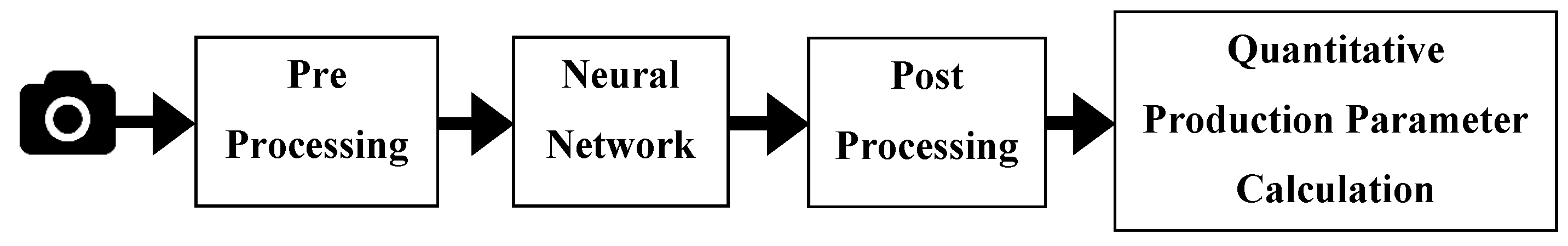
The complete process of determining the PI consists of two fundamental parts: (1) the identification of valid pixels using a neural network for binary classification and (2) a post-processing stage for confirmation or rectification of predictions of pixels. Once the objects have been identified, a valid pixel calculation is made to obtain a number that is proportional to the quantitative production of the hydroponic yield. A pre-processing step can be included to have a better control of the environment captured in the image. Figure 1 shows the complete process proposed in this work.

The entire process is based on the idea that pixels can be discriminated using a neural network as belonging to a target object or not. The neural network is trained with labeled data with valid pixels corresponding to the target and invalid pixels that do not belong to the target. The training is supervised and the discrimination pattern is based on a 3 × 1 array of integers, where the positions in the array correspond to the RGB (Red, Green, Blue) value of a pixel of the image. Once the pixel identification process is over, there will be some false positives and false negatives as predictions are not infallible. To overcome these drawbacks, a post-processing step is performed where the environment of each pixel, referred to as kernel in this work, is evaluated. A scope of a kernel that surrounds each pixel and a siege percentage in the environment are computed to confirm the objective as valid or make the corresponding correction. A siege percentage is defined as the relative number of non-target pixels within a kernel. The general rule of thumb for discriminating pixels is that the probability for a pixel to be valid is determined by the number of valid pixels that surrounds it, that is, a low siege percentage. The values of the evaluation kernel scope and siege levels that determine the validity of a pixel are determined with tests with real data during the implementation of the algorithm. With a count of valid pixels, the PI can then be computed.

In the following subsections, each functional block of Figure 1 is explained. Section 2.1 describes the neural network architecture used in this work and how it was constructed. Section 2.2 describes the post-processing stage of images. Section 2.3 defines the productivity index. Finally, Section 2.4 describes the pre-processing stage of images, which is presented last because it is considered as an optional stage in the entire system.

2.1. Neural Network

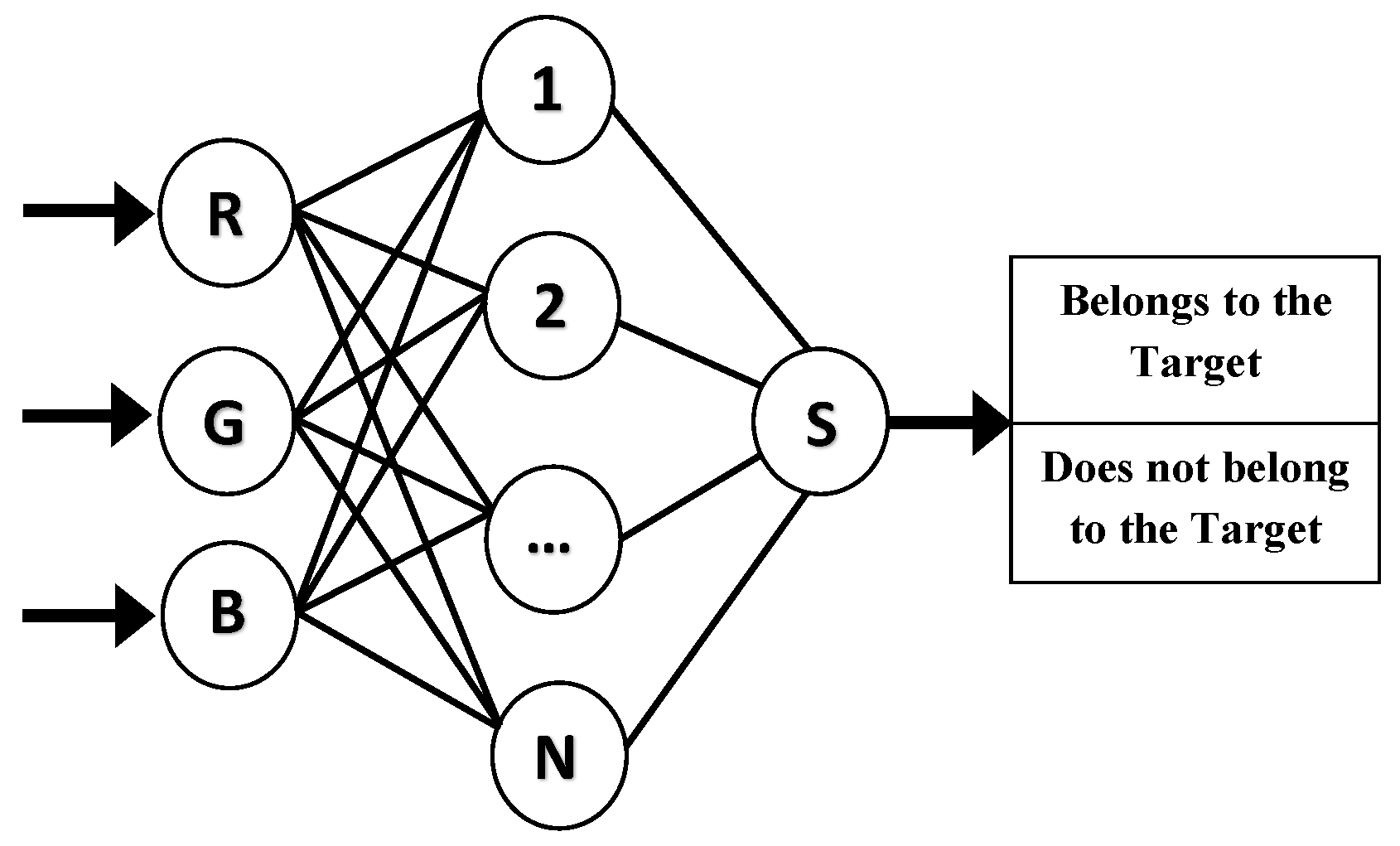
For identification and classification purposes, this work uses a specially designed and trained neural network. The virtues of this computational technique are well known in applications of machine learning [33,34]. In Figure 2, the general outline of the neural network model for a pixel classification process is presented. The pattern to identify is formed by a vector of three components that represent the intensity levels of the red (R), green (G), and blue (B) colors that make up a pixel. The output is binary, that is, it can take only two values or states: “Belongs to the Target” or “Does not belong to the Target,” which makes reference to whether a pixel is part or not of the fruit or vegetable product to be identified in the image. The neural network is a Fully Connected Multilayer Perceptron (MLP), that is, a perceptron-based artificial neural network fully connected between neurons in different layers [6]. No assumptions are made regarding the characteristics of the data; therefore, a fully connected network is used to let the network learn by itself those characteristics through all possible combinations between layers.

The neural network of Figure 2 has a hidden layer with thirty neurons with the aim of achieving the highest percentage of correct predictions with no overfitting; see Section 3.1 for the details of how this number was obtained. The activation function used is ReLU (Rectified Linear Units) for the hidden layer and Sigmoid for the output layer. For training the algorithm, Back-Propagation [35] is used, which adjusts the weights of each perceptron in order to minimize the cost function represented by the mean squared error between the obtained value and expected value contained in the training data. To reach a minimum of the cost function, the optimization technique SGD (Stochastic Gradient Descent) [36] was used, which was iterated over a thousand times to obtain a high percentage of correct predictions in the network. The supervised training was carried out using more than two million registers of data saved in a CSV file (Comma Separated Values).

The data set is divided in two groups, one for training (70%) and the other for evaluation (30%), and it is made of patterns composed of 3 × 1 vectors representing the RGB color intensities of a pixel. Using supervised training, the data is tagged with the correct expected prediction output from the network, a “1” for pixels belonging to the target and a “0” for non-target pixels; see

Table 1. Data set example.

BLUE	GREEN	RED	LABEL
⋯	⋯	⋯	⋯
0	36	19	0
7	46	30	1
34	77	62	0
⋯	⋯	⋯	⋯

for an example.

The numerical values in the first three columns of Table 1 represent the intensity of each RGB component of a pixel, and the last column represents the target (1) or non-target (0) label. Once the training is finished, the network parameters are stored in a JSON data format file (JavaScrPIt Object Notation). Then, in order to identify the target pixels in a new image, it is only necessary to load the parameters of the trained network and run the prediction for each of the pixels. The data set creation process is described as follows.

• Image reading: The first step is the reading of an image file. This is done through the OpenCV library, which allows reading an image file that is then saved in a data structure and manipulated through its predefined methods and functions.
• Component Pixel Path: Once the image has been read, all its pixels are traversed through a programmed iterative cycle. In each cycle, the RGB intensity values of a pixel are accessed and a visual presentation of the analyzed pixel is made via a computer screen for analysis purposes. The numerical values of the RGB intensities receive a labeling from an observer before being stored.
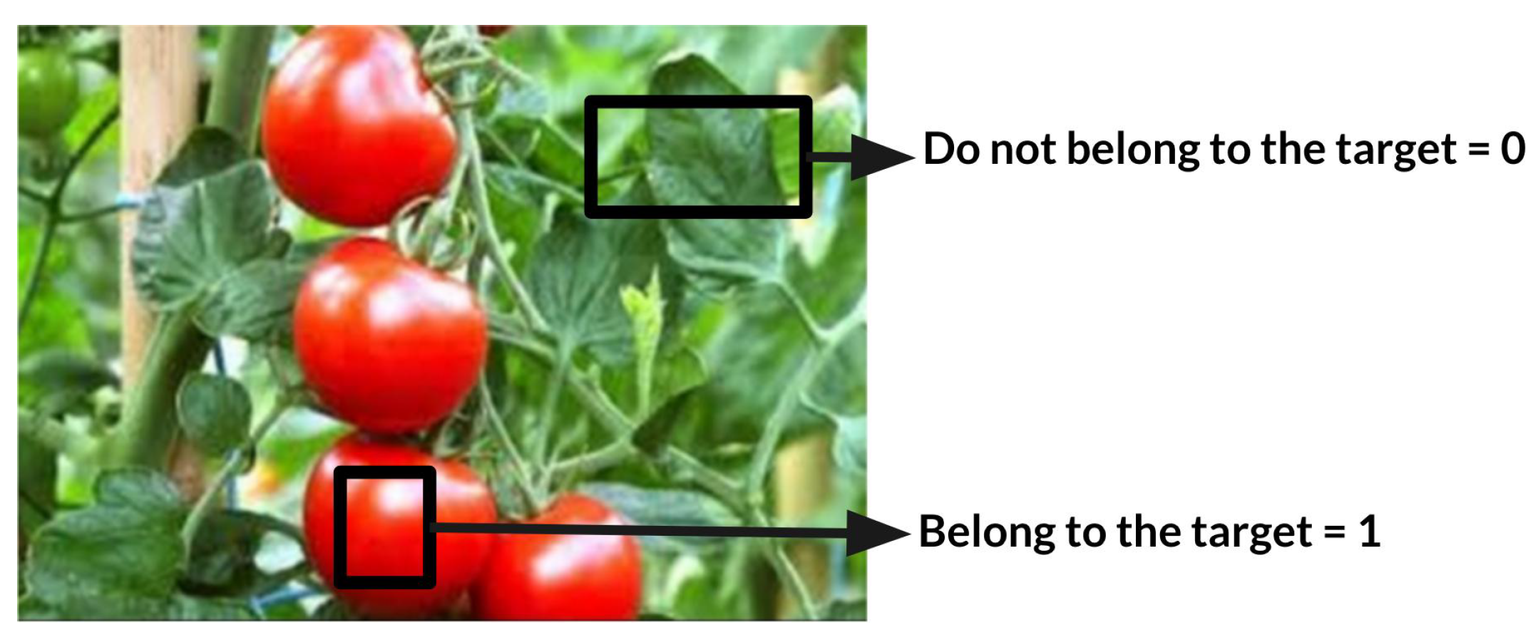
• Visual observation and classification of the pixel: The labeling of the data is done in a “manual”, or rather “visual” way, and depends exclusively on the observer. The desire to implement human characteristics in artificial machines, and for the particular case of computer vision, supervised training requires that the data be pre-classified by a human observer before it is used for training in a neural network. Observing the evaluated pixel of an image, an input is intered by an observer who labels the RGB data trio as belonging to a pixel that corresponds to the target, or not belonging to the target. Figure 3 shows an example of pixel tagging.
• Storage of training vector: Once the RGB data trio is tagged, it is stored in a file inside a non-volatile device. The data thus obtained and stored are then used for training the neural network. It is important to always store data with relevant, diverse, and large amounts of information to improve training and increase the probability of correct predictions by the network.

For the training to be successful, numerous relevant and varied data are needed, i.e., a large quantity of quality data sets of images taken from scenarios of real operations of the system, and with a wide diversification in the nuances of the information to be identified. Once the neural network has been trained with a data set that meets the aforementioned characteristics, it will be ready to make predictions on unknown data and categorize the pixels of new images.

2.2. Post Processing

After making a prediction in the classification of pixels with the neural network in operation after training, inevitably there will be some false positives and false negatives. This problem can be corrected by applying a post-processing step with a verification algorithm proposed in this work. The verification algorithm is based on the idea that a pixel is also surrounded by pixels belonging to the target, and hence, these pixels also belong to the target with high probability. To carry out the verification step, the environment of each pixel of an image is analyzed and a siege percentage is calculated. Siege percentage is an idea that represents the number of pixels different from a given evaluated reference pixel within the analyzed environment of that pixel. If the siege percentage is high, then there is a high probability that the reference pixel is incorrectly labeled after prediction.

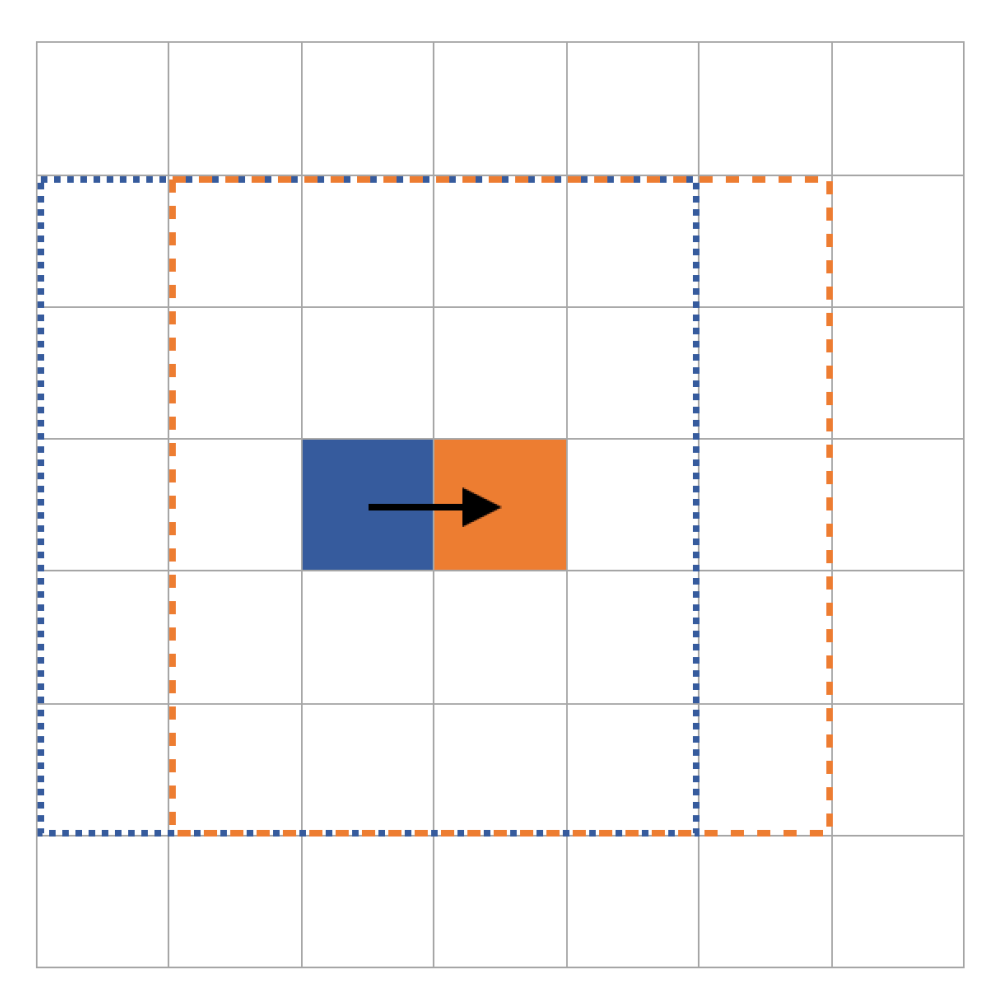
The verification algorithm reads an image pixel by pixel, and each pixel is taken as a reference pixel. The kernel defines the surroundings of a reference pixel evaluated in that iteration of the algorithm. Given a positive integer k, a kernel with respect to a reference pixel is defined as the set of pixels that are contained in a rectangular window of size $(2k+1)\times (2k+1)$ that is centered at the reference pixel. The number k is called the size of the kernel; see Figure 4 for an example. As each pixel in the kernel is examined, the number of pixels different from the reference pixel is counted. This count is interpreted as a percentage, which, if it is equal to or greater than an established siege percentage threshold, then the predicted tag value of the reference pixel is updated. The kernel and siege percentage threshold are established experimentally in this work and will be discussed in later sections.

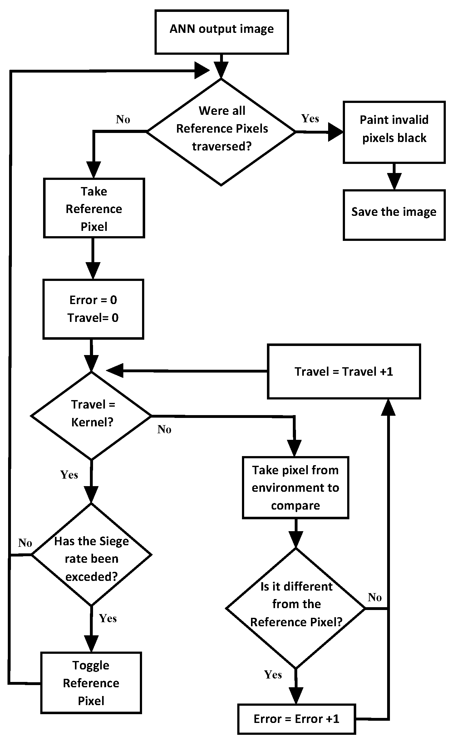
The verification algorithm is shown in Figure 5. There are two main loops, one that goes through all the pixels in the image, and another nested loop that goes through the kernel for each reference pixel. The “Travel” variable keeps track of each pixel in the kernel until the entire kernel is traversed, while the “Error” variable keeps track of the different pixels compared to the reference pixel.

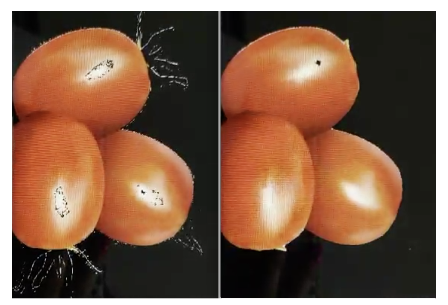
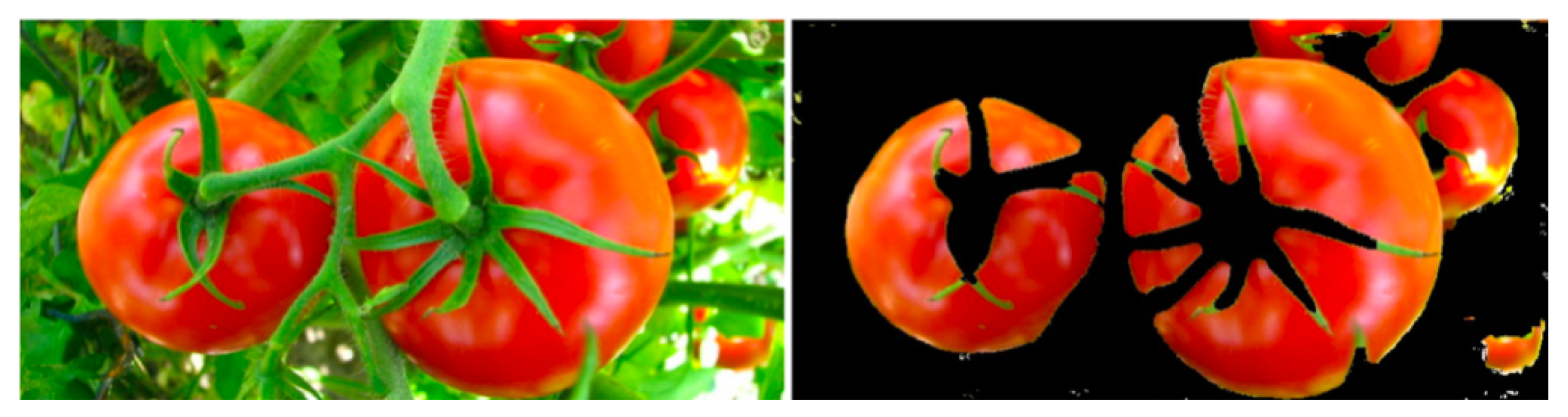
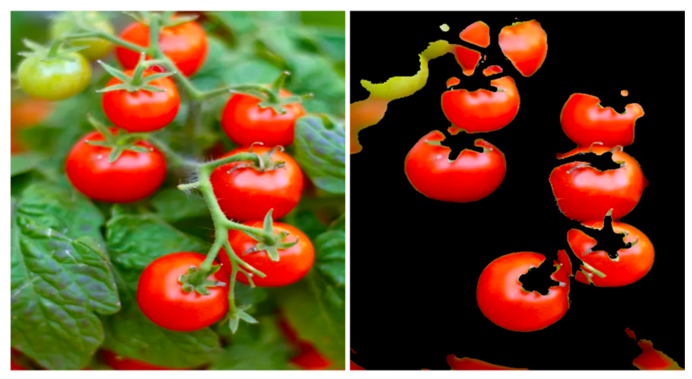
The verification algorithm of Figure 5 validates the pixels identified as belonging to the target and rectifies the false negatives. With a similar argument, false positives can be rectified, that is, correctly labeling a pixel as not belonging to the target when the network wrongly identified it as belonging to the target. Figure 6 shows an example of the neural network prediction and a corresponding post-processed image.

2.3. Productivity Index

To quantify the production of the plots or cultivation tables automatically, a computational production index is defined referred to as a Productivity Index or PI. The PI is defined as a quotient between the number of valid pixels in the image that correspond to a target and the total number of pixels, that is,

$$PI=\frac{\mathrm{number}\mathrm{of}\mathrm{valid}\mathrm{pixels}}{\mathrm{total}\mathrm{number}\mathrm{of}\mathrm{pixels}}.$$

(1)

The process of computing the PI involves traversing all pixels in the post-processed image and counting those labeled as valid pixels, that is, pixels corresponding to tomatoes in this work. The PI is then calculated by dividing the number of valid pixels by the total number of pixels in the image to obtain as a result the proportion of pixels in the image that correspond to the target, which in this work corresponds to tomatoes.

In this way, the PI represents a quantity of tomatoes produced on the plot, that is, a quantitative productivity.

2.4. Pre-Processing

The pre-processing step is explained last because it is an optional functional block of the entire system, and it is only used when there is no physical control of the environment. The environment control refers to the manipulation of everything that appears in the images during the process of taking photographic samples of the crops. The control of the environment can be done manually in the same cultivation site, taking care that everything that appears in the image does not interfere in a correct calculation of the PI. This situation is done by avoiding any foreign object with the same range of RGB intensities as tomatoes, for example, a red tube for irrigation. Some further control of the environment can also be done computationally with a pre-processing step where targets are first identified before performing a classification at the pixel level. The identification of tomatoes can be done with a Convolutional Neural Network (CNN) trained to identify tomatoes [4,37]. A pre-selection of targets with Faster R-CNN focuses the PI calculation only on tomatoes, thus avoiding any foreign object that may introduce errors in the calculation of the PI.

Table 2. Faster R-CNN hyperparameters.

Hyperparameter	Value
Anchor box scale	[0.25, 0.5, 1.0, 2.0]
Anchor box aspect ratio	[0.5, 1.0, 2.0]
Anchor box height stride	16
Anchor box width stride	16
Iterations	200,000
Learning rate	0.0003
Momentum for SGD	0.9

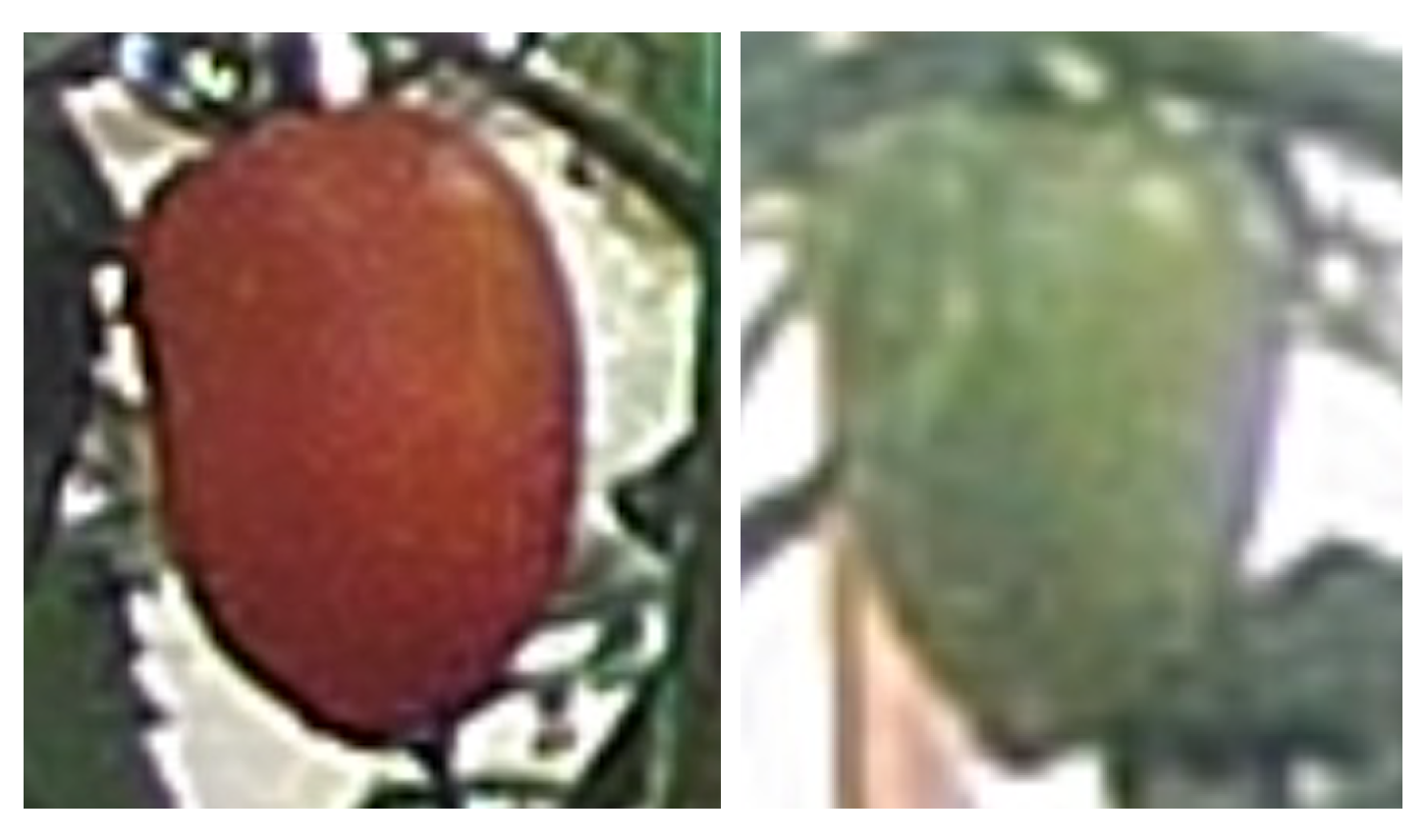
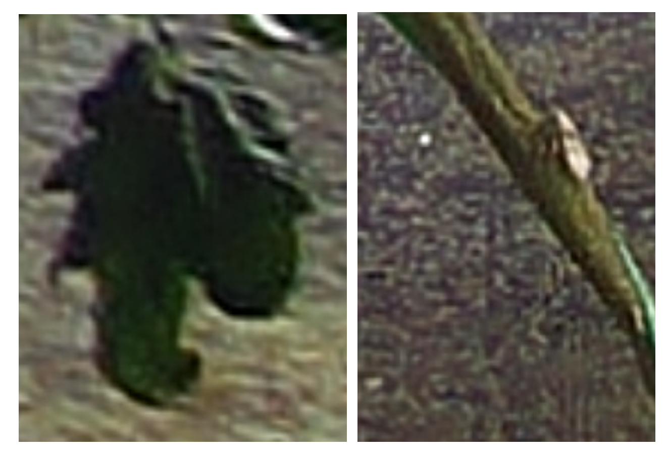
shows the hyperparameters for the Faster R-CNN with a ResNet architecture [38]. Figure 7 shows some examples for the valid targets training data set and Figure 8 for the invalid targets training data set.

3. Results

The essence of this work lies on identifying whether objects in an image are tomatoes or not. The main goal is to quantify valid pixels in the image, thus obtaining an indicator or index of production quantity. The computational implementation is done with the programming language Python version 3.6, along with its libraries for scientific computing applications: Keras in its version 2.2.4 for neural networks, and OpenCV in its version 4.1 for digital image management.

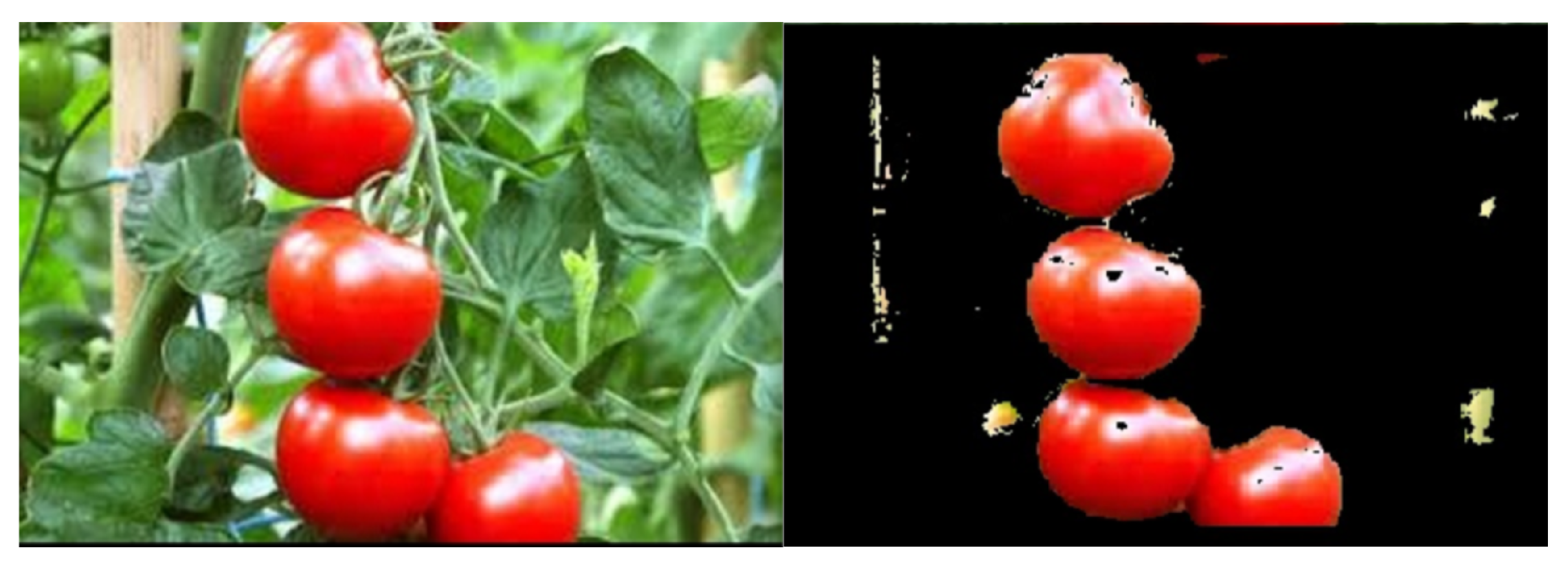
Figure 9 shows results of the behavior of the trained neural network. Invalid pixels are painted in black and valid target pixels are displayed. As can be seen in Figure 9, the prediction is not perfect and false positives and false negatives appear, that is, pixels identified as valid targets when in fact they are not, and pixels identified as invalid when in fact they are. The post-processing verification algorithm can check these predictions and rectifies them.

3.1. Siege Percentage Threshold, Kernel Size, and System Error Rate

To calculate the precision and accuracy of the models and obtain a fair estimation of the siege percentage threshold and kernel size, it is necessary to find the deviation between the observed values and the real values. For this purpose, an image is “manually painted”, simulating the ideal detection of the pixels corresponding to “tomatoes.” This way, the manually painted image can be used as a reference to measure different pixels when the post-processed image and the ideal image are compared against each other. Thus, a pattern for calculating the system’s error can be established. Figure 10 shows an example of an original image and its respective ideal detection pattern.

Several tests have been carried out to choose the best combination of post-processing parameters and the neural network model with the least prediction errors. The kernel size, the siege percentage threshold value, the number of hidden layers of the neural network, and the number of neurons per layer have been varied. Figure 11 shows the test results for the calculation of the average error of the processing of 200 samples with a neural network model with a single hidden layer of 30 neurons. The error rate is calculated as the number of pixels different from the ideal pattern in relation to the total number of pixels of a image.

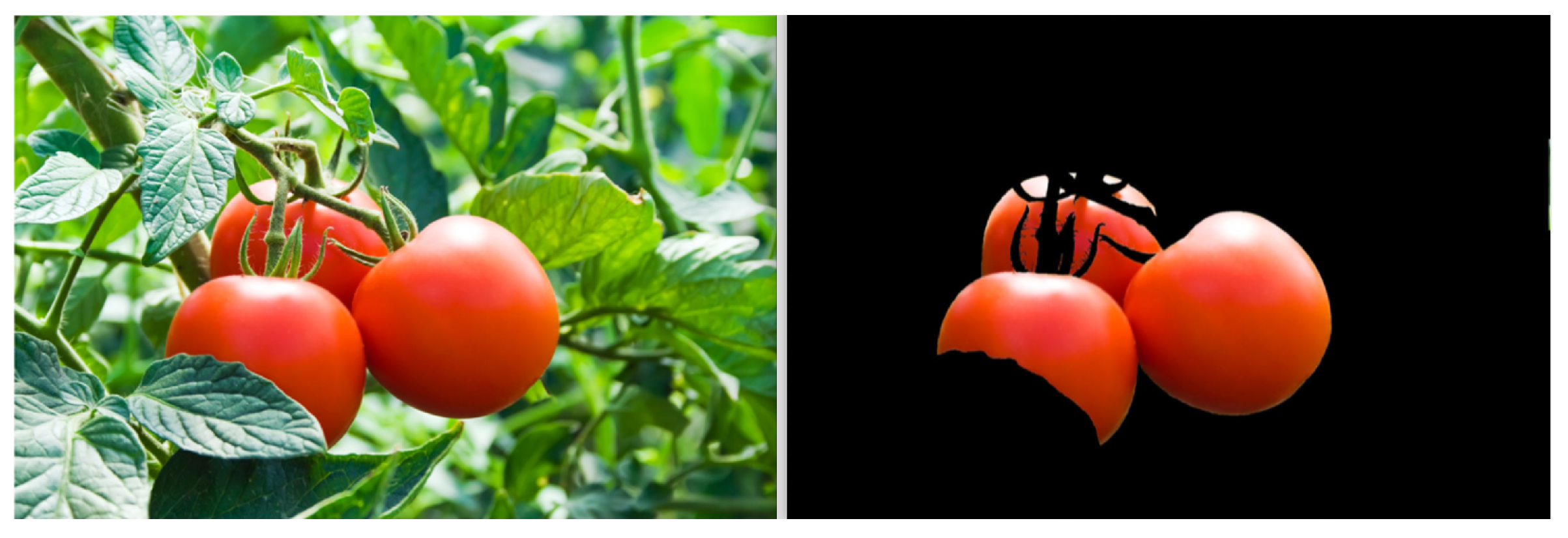
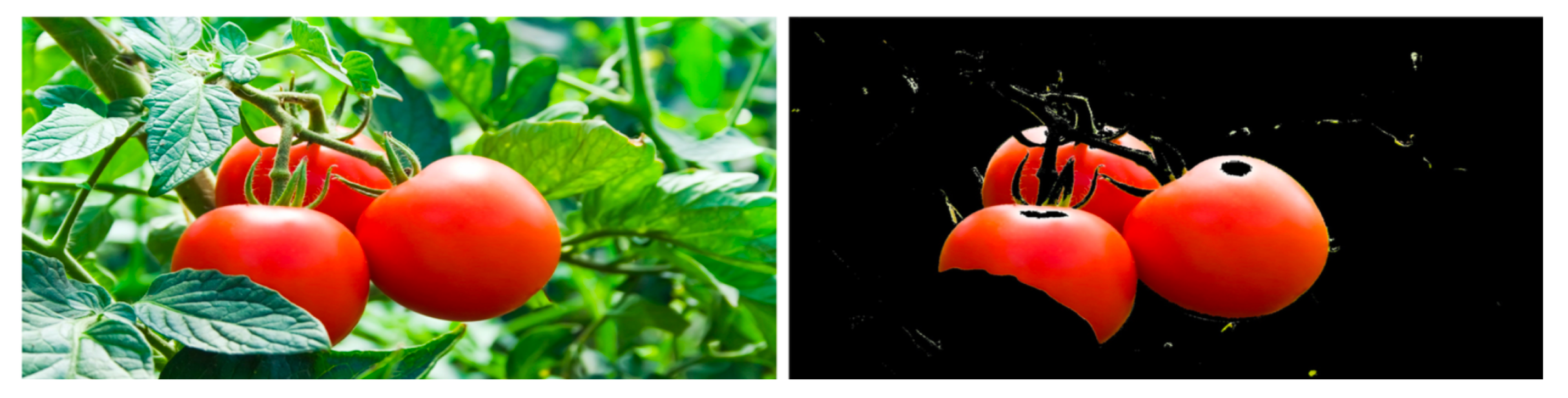
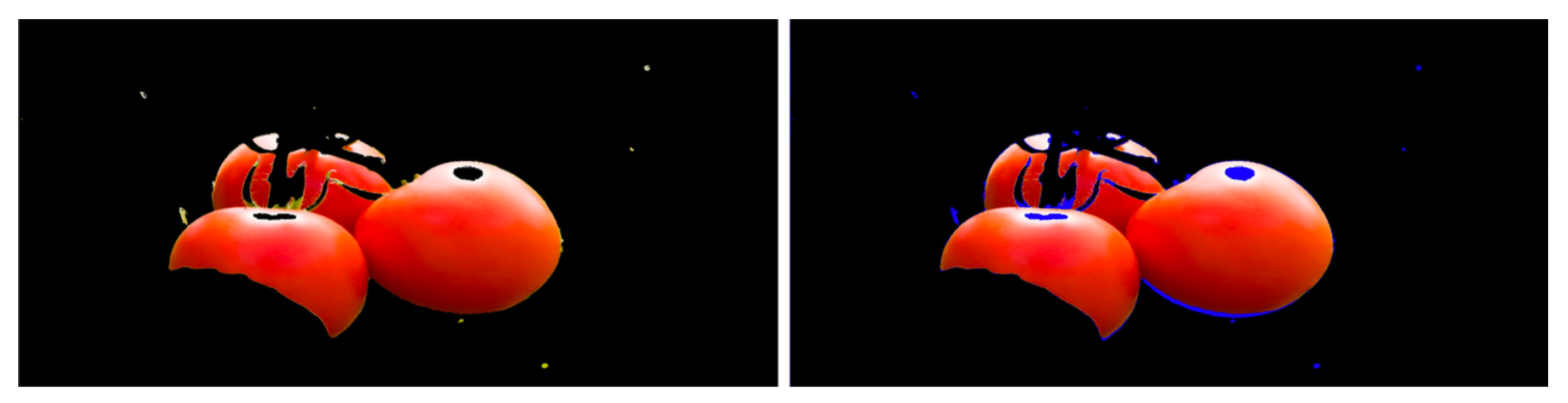
The kernel size and siege percentage threshold values with the minimum system error rate that are used in this work are a kernel size of 10 pixels and a siege percentage threshold of 60%. Figure 12 and Figure 13 show each step of image processing. Figure 14 and Figure 15 also show two examples of a final result after all processing stages.

3.2. Application of PI on a Complete Tomato Growing Season

Once the PI is computed for each image of the crop plot sampled over time, a time curve is obtained that describes the growth of cultivated products and allows objective comparisons between agricultural plots.

For this work, tomatoes were grown in a hydroponic greenhouse in three different plots, each with a different nutrient dosage. The concentration of the final nutrient solution was modified from a commercial solution based on the Hoagland solution [39]. Plot 1 received the commercial nutrient dosage of 100%, plot 2 with a diluted dosage of 75%, and plot 3 received a diluted dosage of 50%. Using the PI, it is possible to determine whether a diluted nutrient solution affects the quantitative production of the plots. Then, it is another goal of this work to establish an optimal dosage for greater effective production.

Since the sowing of tomatoes, photographs were taken of the plots with a sampling period of one day, and images were always taken from the same distance as recommended by the proposed method, which was 1 meter in this case. Additionally, each plot was divided into 8 subplots to cover the entire extension of the crops. The length of the plot is 16 meters approximately, and photos were taken along the plot from both sides. The PI resulting from a complete parcel in a single temporal sample event is the result of the average PI for each sub-parcel and the average PI of both sides. The temporal registration of the PI is represented through curves that will be shown later as results and that will serve to analyze and compare the different production techniques.

In summary, the PI is calculated each day for each of the three plots, and for each day 16 photographs are taken, since there are 8 subplots and one photograph is taken from each side. This gives us a total of 48 photographs; thus, the PI for a day is computed by averaging the PI of each individual photograph.

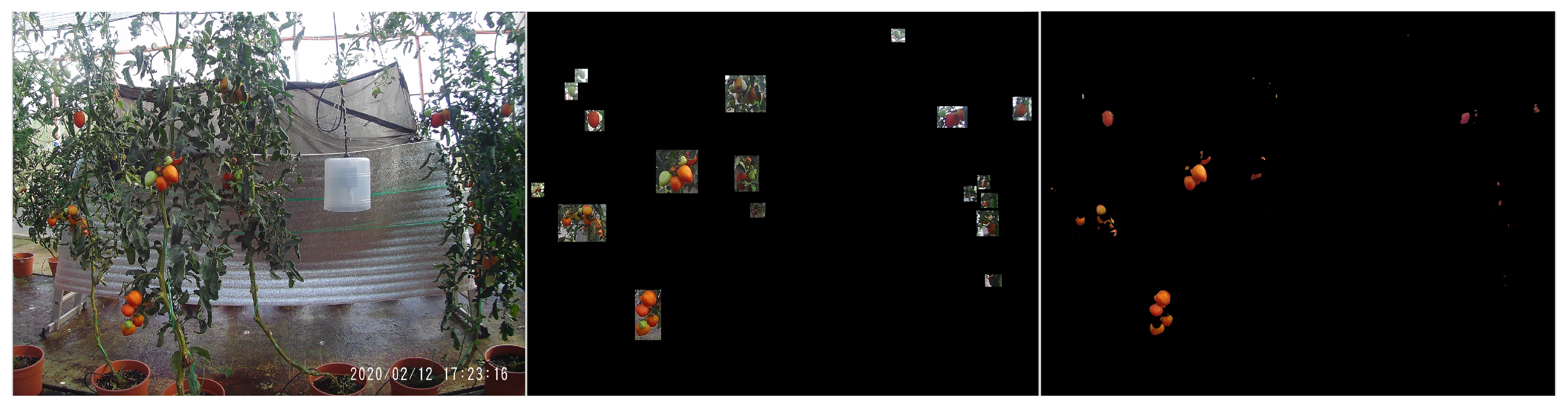
Digital images are in JPEG format with a dimension of 5120 × 3840 pixels encoded in 8-bit RGB per channel. The digital camera used was an AKASO Brave 4 4K 20MP. As an example, Figure 16 shows the original image of one sample, the pre-processing with CNNs, and its processing with the proposed method identifying objective pixels.

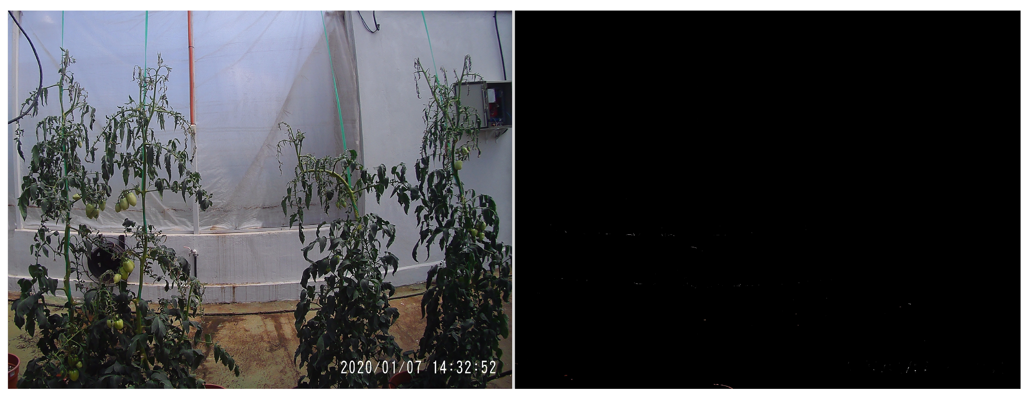
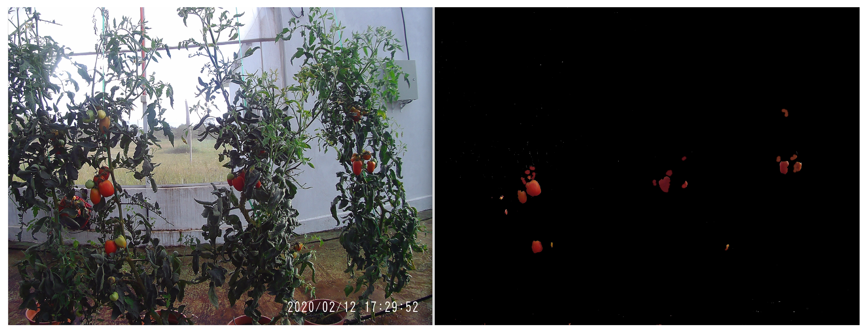
Figure 17 and Figure 18 show the photographic samples and the digital processing of the first sampling event and an intermediate event, respectively. The processing of the first sample in Figure 17 presents a totally black screen, indicating that the target is not perceived with the algorithm. Over time, tomatoes begin to ripen, and the target is identified by computing the PI, as shown in Figure 18, thus achieving a record of growth and productivity through the PI curves. Daily photographic samples were taken from sowing to harvest, and the resulting PI processing gave rise to a time curve that determines the growth of tomatoes and describes the evolution of quantitative productivity.

A drawback that occurs when calculating the PI over time is what is called, in the context of this work, as the Harvesting problem, which influences the accuracy of the PI calculation as time passes. An early harvest can cause the PI measurement at that moment to drop when, in reality, the productivity is the same or increases, that is, productivity measurement errors are introduced due to the extraction or fall of very mature targets. In order to overcome the harvesting problem, a method of accumulating the PI is proposed according to

$$PI{\left(accumulated\right)}_i=\sum _{n=1}^{n=i}\Delta P{I}_n\mathrm{where}\Delta P{I}_n=P{I}_n-P{I}_{n-1}>0,$$

(2)

and $P{I}_n$ is defined as the instantaneous PI at time step n. The time curve of PI actually shows the accumulation of PI over time, which translates into cumulative productivity regardless of whether the instantaneous calculations record a PI reduction due to early harvest. The accumulated PI at a given instant i is calculated with the sum of $\Delta P{I}_n$, from the first sample to that of instant i, as long as $\Delta P{I}_n$ is positive. Thus $\Delta P{I}_n$ represents the difference of instantaneous PIs between consecutive samples. The value of $P{I}_i-P{I}_{i-1}$ must necessarily be positive in order to be included in the summation, since a negative value represents an early harvest, and, after it is identified in this way, it must be ignored in the calculation to avoid incurring productivity measurement errors.

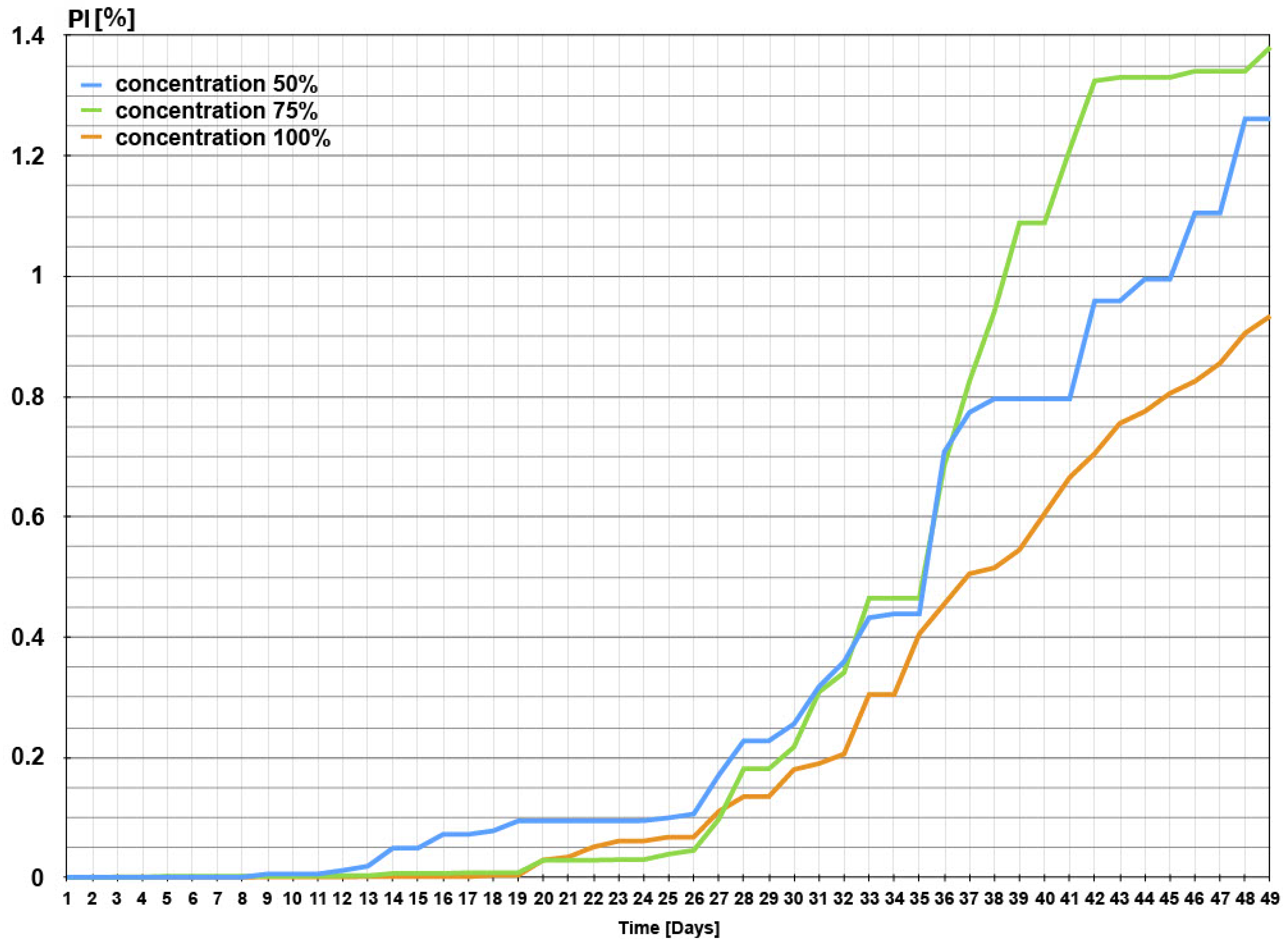
The calculation explained in the previous paragraph was performed with the three plots, and the resulting curve is presented in Figure 19.

Looking at the time curves of the three plots, relevant information regarding their productivity can be obtained. In the first stage of growth, it is observed that a nutritional solution at 50% shows higher productivity, even reaching 23.5 times more production than the plot with 100% nutritional solution on day 19, and it is also 11.2 times more productive than the 75% plot on the same day. In the middle time stages, the productive superiority of the solution is maintained at 50% with respect to the others until day 33, in which the 75% solution begins to look more productive; meanwhile, the 100% solution stays very inferior. In the final stages, the 75% and 50% solutions show higher productivity than the 100% solution, these being 1.5 and 1.4 times more productive, respectively. The 75% solution presented the highest final productivity, being 1.1 times more productive than the 50% solution.

Table 3. Count, weight, and PI comparison table.

Solution	Count [units]	Weight [g]	PI [%]
Concentration 50%	73	4299	1.26
Concentration 75%	89	5867	1.38
Concentration 100%	60	3997	0.93

shows three types of productivity magnitudes for the three plots in their final stages, two of which are commonly used, like weight and count, and the third which is the PI proposed in this work. As can be seen, there is a certain correlation between the three magnitudes, where all of them reflect the superiority of the solution with 75% concentration, followed by the solution at 50%, and the solution at 100% with the slightly worst productivity.

It is interesting to note that the 75% solution is 1.5 times more productive than the 100% solution, taking into account the three specified magnitudes. However, if we compare it against the 50% solution, it is 1.2 times more productive considering the count, 1.4 times more productive considering the weight, and 1.1 times more productive considering the PI. This difference, even between two well-known measures of productivity, is due to the precision with which all these magnitudes measure the produced quantity (two large tomatoes are heavier than two small tomatoes). The PI approach aims to be more precise than the most common approach in computational vision where objects counts are implemented. The PI aims to improve even measurement by weight, automating quality control through pixel-level identification of healthy targets (one kilogram of healthy tomatoes and one kilogram of rotten tomatoes have the same weight) and making it easier to track the growth of tomatoes instead of doing it through weighing before harvest.

4. Discussion

The productivity index or PI was implemented using digital image processing with a perceptron-based artificial neural network. It should be noted that the calculation of the PI is made based on photographs taken automatically by a robotic system or by a human that acquires digital samples always from the same distance and pointing to the same objective. This way, the automatic system creates the necessary context for the PI to make sense and be able to provide necessary information regarding the growth of agricultural products in the different plots. The PI also provides a computational numerical parameter for comparisons between different crops and their agro-production techniques, such as composition and dosage of nutrients, thus obtaining a reference for optimizing production.

Regarding the precision in the identification of objects in digital images, Reis et al. [32] achieves a precision of 97% in the identification of red grapes using a pixel identification method similar to this work. Villacrés and Auat [4] were able to identify cherries with a precision of 85% using faster R-CNN. Si et al. [13] identified apples using stereoscopic vision with a precision of 89.5%. Xiang et al. [15] achieved a precision of 87.9% in the identification of groups of tomatoes using binocular stereo vision. Zhao et al. [14] showed that, combining the AdaBoost classifier and color analysis, tomatoes can be detected with a precision of 96%. With the Single Shot Detector, (SSD) the authors of Reference [40] showed a precision of 95.99% in the detection of tomatoes. Other works, like Mu et al. [41], achieved a precision of 87.83% using faster R-CNN, also in tomatoes. In this work, a specific neural network was trained for the identification of pixels belonging to tomatoes and a verification algorithm was programmed to optimize target detection achieving a success rate of 98.93%. The nature of the computational technique used to calculate the PI allows to be adapted for other scenarios and contexts. With the versatility of neural networks, the same concept developed in the present work can be applied to detect other fruit and vegetable species simply by retraining the network with another specific data set for the desired target crop.

Other works in the literature, besides identification, use the count of objects as productivity parameter [4,14,40,41,42,43]. As explained before, counting of objects is not a precise indicator for productivity, and that is one reason this works introduces the PI. Most of the works in the literature focus on detecting objects and not on monitoring of objects, which is what this current paper is emphasizing. For monitoring, there are works that keep a register of the size of plants [20], controlling diseases [44], environmental control [11], tracking the count of flowers and tomatoes [40,45], and keeping a registry of the volume of tomatoes [46]. This last work of Fukui et al. [46] is the closest to the current paper, and one important point to notice is that the authors of Reference [46] achieved good results in a controlled environment inside a laboratory, whereas, in outside environments, the results were not as expected. On the other hand, the results obtained in this work were performed completely in a typical working environment of hydroponic tomatoes.

The PI was computationally applied over time through digital image processing with a fully connected multilayer perceptron in three tomato crop plots and three different nutrient dosages of a Hoagland solution. The control of the environment of the sampling place was analyzed, and a computational method based on convolutional neural networks was proposed to avoid erroneous measurements. In addition, an adequate mathematical calculation was established to correct the Harvesting Problem caused by early harvests during the processing of the curves. Through the innovative computational method of PI calculation, three time curves of three different production techniques were obtained: dosing of nutrients with commercial chemical compounds at 100%, diluted at 75%, and diluted at 50%. With these time curves, the production of the plots was recorded and analyzed. As a conclusion, it was observed that the plots with a nutrient dosage diluted to 75% showed higher productivity compared to the other two plots with different dosing techniques, this being 1.1 times more productive than the plots with a dosage of 50% and 1.5 times more productive than those with a dosage of nutritional chemical compounds at 100%. The PI was compared with two well-known magnitudes of productivity, weight and count, highlighting the advantages of this approach in precision and automation of quality control.

In agronomic terms, it can be concluded through the PI that there is no significant difference in productivity between the three solutions studied. Therefore, the results suggest that it is recommended to use a 75% solution to have a slight improvement in productivity, as well as to potentially use a 50% solution to minimize production costs.

5. Conclusions

This work introduced a new computational parameter, a so-called Productivity Index or PI, to quantify productivity of hydroponic tomatoes using neural networks and digital image processing. The neural network presented an error rate of 1.07% in the identification of pixels belonging to tomatoes. This neural network together with the PI was then used in a full season of hydroponic tomatoes in order to test the entire system in a real working environment. From the application of the PI in real scenarios, it is possible to conclude that there is no difference in terms of productivity of a plot of tomatoes when a Hoagland solution is diluted 50% with water or is not diluted at all.

One limitation of the approach is the poor detection of very green tomatoes, which requires specializing the system for the detection of tomatoes before their middle ripening stage. The neural network of this work is trained to detect tomatoes when they start its red coloration process; when tomatoes are green they are not perceived by the network, which will required a new training stage to detect green tomatoes and can potentially be confused with invalid objects like leaves. This, however, can be considered as positive, since the system can detect which exact moment in time a tomato plot enters its ripening stage by observing the change in PI.

Regarding occlusions, two types can be noted: occlusions by invalid targets (branches, leaves), and occlusions by valid targets (tomatoes obstructing other tomatoes). Invalid target occlusions can be improved with good environmental control, periodic pruning, or human intervention. Payne et al. [43] takes images from four different points of view pointing to the same objective in order to obtain robust results even with occlusions. In this paper, the photographs were taken only from two points of view considering that plots are organized in lines. The proposed method of this work, however, offers improved solutions of up to 50% in invalid target occlusions. This is due to the way samples are taken and the process of computing the PI, that is, the samples are taken from both sides of the crop line and the resulting PI from that subplot is calculated by averaging the instantaneous PI of the image from each side of that subplot. Having two points of view facing each other improves the field of vision when taking samples. Occlusions for valid objectives are more complicated to solve, and they are beyond the scope of this work, which is why it is proposed to study them in future works. The solution in general is to identify tomatoes that are occluded, define their contours, and reconstruct them with an elliptical approximation. Small occlusions in general are accepted and tolerated since they do not affect the PI when using it as a means of comparison. This is because small occlusions can be considered as “white noise” that affect all measurements equally.

The execution time of the entire process is approximately 3 minutes for each image. A dedicated server was used in this work that stores the images and processes them per day. Execution time can be reduced by implementing GPU (Graphics Processing Unit) processing, thus parallelizing calculations. To achieve this, the program code must be adapted to implement the same algorithm presented in this approach. One of the advantages of using a neural network as a classification method is its ease of parallelizing calculations with GPU programming. This implementation will be done in future works in order to improve the system.

For future work, this study with image processing is intended to be validated with other agronomical studies of the productivity and the physicochemical properties of crops. Even though this work used Faster R-CNN, which is considered as a deep neural network, further studies using other network architectures can improve our understanding of the applications of deep learning for the detection and classification of fruits and vegetables. Furthermore, it is expected to use optimization algorithms, like genetic algorithms, in order to improve the model of the neural network.