Load and Unload Technology to Improve Round-Bale Hauling Efficiency

Abstract

There are two key parameters in short-haul truck operations to deliver biomass to a biorefinery: (1) mass of the load and (2) cycle time (load, travel, unload, and return). A plan to optimize both these parameters is outlined in this study. Operation of a logistics system to deliver 20-bale racks to a biorefinery for continuous 24/7 operation, 48 weeks/year is described. Round bales are stored in satellite storage locations (SSLs) by feedstock producers. A truckload consists of two tandem trailers (40, 0.4 Mg bales), a specification that maximizes load mass. Load-out at the SSL (loading bales into racks) is performed by a contractor and paid by the biorefinery. Subsequent hauling (truck tractor to pull the trailers) is also contracted for by the biorefinery. Central control is specified; the “feedstock manager” at the biorefinery decides the order SSLs are loaded out and can route a truck to any SSL where a load is ready. Tandem trailers with empty racks are dropped at the SSL, and the trailers with full racks are towed to the biorefinery. Uncoupling the loading and hauling in this manner reduces the time the truck waits for loading and the SSL load-out waits for a truck; thus, productivity of both operations is increased. At the biorefinery receiving facility, full racks are removed from the trailers and replaced with empty racks. The objective for this transfer is a 10 min unload time, which completes a logistics design that minimizes cycle time. A delivered rack is placed in a rack unloader to supply bales for immediate processing, or it is placed in central storage to supply bales for nighttime and weekend operations. Three biorefinery capacities were studied: 0.5, 1.0, and 1.5 bale/min. The analysis shows that rack cost to supply a biorefinery processing a bale/min for 24/7 operation is ~3.00 USD/Mg of annual biorefinery capacity, and the rack trailer cost is ~3.25 USD/Mg. Total delivery cost, beginning with bales in SSL storage and ending with a rack being placed in an unloader to deliver individual bales for processing, is 31.51, 28.42, and 26.92 USD/Mg for a biorefinery processing rates of 0.5, 1.0, and 1.5 bale/min, respectively.

1. Introduction

This study analyzes a conceptual design for a facility that receives truckloads of round bales for continuous annual operation of a biorefinery. “Biorefinery” means any processing system by which biological feedstocks are converted to useful products, no matter what the products and no matter what types of processing are used (biological, chemical, thermal, or a combination). Specific parameters were chosen for a biorefinery located in the Piedmont, a physiographic region across five southeastern states USA (Virginia (VA), North Carolina (NC), South Carolina (SC), Georgia (GA), and Alabama (AL)). The feedstock is switchgrass (Panicum Viragos L.), a native warm season perennial grass well adapted to the rainfall patterns and soil types in the region. The proposed biorefinery business plan envisions that feedstock producers will receive contracts to grow, harvest, and place round bales (1.5 m diameter, 1.2 m long) in satellite storage locations (SSLs) with access for load-out and highway hauling.

A rack system for hauling round bales has been described [1,2,3,4]. The overall concept envisions that the biorefinery will contract for the loading of bales into racks at the SSL, a contract hereafter referred to as a “load-out operation”. The biorefinery will operate a fleet of truck tractors to pull rack trailers and deliver for year-round operation.

This study has two main interconnected objectives: (1) highlight the fact that the two main parameters to optimize hauling in the logistics system are load-out productivity and truck productivity and (2) advocate for central control of feedstock delivery.

1.1. Lessons from the Cotton Industry

Much can be learned about the needed logistics for a biorefinery by studying the current cotton industry [2,5]. Producers contract with a specific gin to gin their cotton (convert seed cotton into bales of clean fiber for year-round delivery to a textile mill). With the cotton module system, producers build modules (compacted blocks of seed cotton) at the edge of a harvested field where there is access for a self-loading truck (module hauler). Hauling of the seed cotton to the gin is part of the contract between the seed cotton producer (i.e., feedstock producer) and the gin (i.e., biorefinery). Modules are protected with a water-repellent cover and can be left in field-side storage (satellite storage) for later delivery, or they can be set down in the gin’s (central) storage and removed as needed to establish a continuous supply into the gin.

A self-propelled cotton harvester, which bales seed cotton, was introduced in 2007. This machine round bales the cotton, wraps these bales in solid plastic, and places them along the edge of the field. The harvester forms a bale in the bale chamber while wrapping the previous bale. It does not have to stop to eject a bale, and it provides the needed in-field transport to the edge of the field where the wrapped bale is ejected. These bales (2.1 m diameter, 2.4 m long) are loaded with an all-terrain forklift onto a standard flat-bed truck trailer for transport. In some cases, the hauling is provided by the producer, and in some cases, it is provided by a trucking company under contract to the gin.

1.2. Multi-Bale Handling Unit for Large Rectangular Bales

A prototype self-propelled in-field hauling unit, identified as a bale wagon, was developed by [6] for large rectangular bales (1.2 m × 0.3 m × 2.4 m). This machine accumulates 6 bales into a block 3 high by 2 wide and transports this block to the edge of the field where it is placed on the ground. Once 36 bales are accumulated, the full load is transported. The tractor-trailer truck used for the hauling has a trailer that can tilt, and a drive track that engages the ground and pulls the truck back under the 36-bale block to load it [6]. This handling system emulates the cotton module system in that the truck can self-unload at the biorefinery by directly placing the 36-bale module on the inlet conveyor into the biorefinery or by setting the module on the ground in central storage to be picked up by the same live-bottom truck and delivered to the conveyor to maintain a continuous input for nighttime and weekend operation.

The large-bale hauling system could have applicability in a region where large rectangular bales are practical and widely used. The prototype bale wagon is 2.9 m wide; therefore, movement on the highway from field-to-field is problematic, particularly in the Southeastern USA. The current commercial technology is the “Stinger” (https://stingerbiomass.com/), a self-propelled machine that self-loads large rectangular bales and stores these bales six high by tilting the bed and placing the stack adjacent to previous stacks. One model of the Stinger can also self-load large round bales (1.8 m diameter, 1.5 m long) and unload them into single layer storage.

1.3. Hauling Controlled by Biorefinery

A biorefinery located in the Piedmont will want to contract with as many surrounding producers as possible to increase the “feedstock density”, defined as Mg/km² and thus reduce the average USD/Mg hauling cost. The potential feedstock contractors are small- and intermediate-size farmers; thus, they are not capitalized to purchase specialized equipment for a biomass contract. This constraint defines two operational parameters:

• The round bale is the handling unit because the round baler is the predominant machine used to harvest forages for current livestock enterprises. No new harvesting equipment has to be purchased to obtain a feedstock contract.
• Hauling (load-out from SSLs and delivery to the biorefinery) is the responsibility of the biorefinery. Capitalization for the specialized (high productivity) equipment required is more readily available to the biorefinery; plus contracts can be granted for year-round hauling, which make the contracts attractive to small businesses, for example, a trucking company with a small fleet of trucks.

The advantage gained with central control of hauling was documented by Aguayo et al. [7]. They developed a method for scheduling shipment of bales of corn stover from actual road-size storage locations in the Midwest USA. Their method reduced average hauling cost about 20% over the reported hauling cost, where hauling was performed in the order field harvest was called in.

1.4. Importance of Receiving Facility

The design of a receiving facility is a critical component in the logistics chain that supplies feedstock for continuous annual operation for any biomass industry. Receiving facilities for some current agricultural and forest-product industries is designed to receive random feedstock deliveries from their feedstock producers. When deliveries are not evenly distributed, trucks wait in a queue to be unloaded. Current well-designed receiving facilities weigh in, unload, and weigh out trucks as quickly as possible to minimize wait time. Minimizing turn-around time increases average truck productivity (Mg/d), which minimizes truck cost (USD/Mg).

1.5. Central Control of Hauling

This study presumes the central control of hauling as outlined by Grisso et al. [3]. Two 20-bale racks on tandem trailers form a 40-bale load. The biorefinery purchases the feedstock in the SSL and schedules the delivery. Control of all hauling is conducted by a “feedstock manager” at the biorefinery. With communication on the location of all trucks and the operation at all SSL load-outs, this manager can dispatch any truck to any SSL where a load is ready for transport.

Rack loading at the SSL is uncoupled from hauling to minimize the time trucks wait to be loaded. The proposed business plan is as follows: a separate contract pays the load-out contractor, and these contractors are in continuous contact with the feedstock manager. Projected time when a load is ready is relayed over the cell phone network, or organized through a GIS-based network analysis web service; thus, a truck arrival can be scheduled as soon as possible to minimize wait time by the load-out operation. A truck arrives at the SSL, and the operator unhooks the tandem trailers with empty racks and hooks the waiting tandem trailers with full racks. The specified transfer time from empty to full load is 15 min.

1.6. Storage Advantages of Rack System

Storage can add significant cost to any feedstock logistics chain. Three storage features (field, SSL, and central) are available in the “Rack System”, and these provide for needed flexibility.

The first storage feature, in-field storage, is available with round bales because the rounded top sheds water, and the bales can be left in the field for a short time (days) before in-field hauling. This in-field storage provides the advantage of uncoupling the harvest and in-field hauling operations and thus provides an opportunity for improving the cost efficiency of both operations.

The second storage feature, satellite storage (SSL), provides the needed transfer point between in-field hauling and highway hauling. It is expected that the distribution of SSLs will be chosen to constrain the Mg-km parameter (field to SSL) to less than 5 km. This means that, averaged across all Mg stored at a particular SSL, each Mg will be hauled less than 5 km from the production field to the SSL. This constraint gives the feedstock contactor a limit for their in-field hauling distance and thus defines their in-field hauling cost and time. It also means that the system may have a large number of different capacity SSLs to match the field capacities.

The third storage feature, central storage, provides a feedstock buffer at the biorefinery. A biorefinery, like many other industrial plants, would like to operate as close as possible to just-in-time (JIT) delivery of their raw material, as this gives them the lowest cost for their operations. If JIT is not possible, they want the smallest at-plant inventory for cost-effective operation of their plant. There is an obvious trade-off in the logistics system design between the higher cost to insure JIT delivery and the cost of central storage.

The rack system concept must include some central storage, even though known quantities of feedstock are stored in a known network of SSLs, and the feedstock manager is controlling the deliveries. The size of the central storage depends on the number of days that deliveries are delayed, due to ice and snow in winter and heavy rain during any season. The penalty incurred when the biorefinery runs out of feedstock is the critical variable. The biorefinery may decide it is cost effective to allow some “turn-down” for short periods in order to gain a cost reduction in the operation of central storage. This variable is set by the biorefinery business plan, and is not defined for this study.

1.7. Elimination of Single-Bale Handling

With the concept presented here, the bales stay in the rack until processed—there is no individual bale handling at the biorefinery. This design feature is consistent with other herbaceous biomass industries. Cotton stays in the handling unit, module or large round bale, until it is ginned. Sugar cane remains in bins for short-term central storage until it is processed during nighttime operation.

This reduction in bale handling not only reduces cost but also reduces damage to the bales. Modern baling equipment produces a bale with higher density; in addition, multiple wraps of net do a good job of stabilizing the bale. However, even with storage on a crushed gravel surface in the SSL, there is some deterioration in storage, particularly when storage is 6 months or more. Using the operations plan presented here, individual bales are handled only once, when they are placed in the rack during load-out.

2. Constraints Used for This Analysis

• Feedstock production area for a given biorefinery is defined as a 50 km radius. This constrains the haul distance and thus truck cycle time.
• Load-out operations at the SSLs will be 10 h/d, 6 d/wk.
• Average truck productivity (Mg/d) is computed using a truck (i.e., truck tractor) cycle time based on the average travel distance across all SSLs.
• A truckload is two tandem trailers with one 20-bale rack on each trailer and 40 bales/truckload.
• Receiving facility operations will supply the biorefinery 24 h/d, 7 d/wk. Normal operations specify that truck deliveries begin at 0600 and end at 1800 h, 6 d/wk.
• Continuous 6 d/wk operations are assumed for load-out, delivery, and receiving facility operations excepting delays due to hard rain, sleet, and snow. Achieved productivity parameters are defined by reducing ideal (theoretical) productivity parameters to account for delays.
• Central storage at the receiving facility is set at a maximum of 3 days, meaning the biorefinery can operate at full capacity for 3 days with no deliveries. This constraint is set considering potential consecutive winter days when roads are impassible in the Upper Piedmont (VA, USA).

3. Analysis Procedure

Example calculations are presented here for a “baseline” biorefinery processing rate of 0.5 bale/min, 24/7. The required weekly deliveries are (0.5)(60)(24)(7) = 5040 bales/wk. For bales averaging 400 kg, the biorefinery is processing 2016 Mg/wk. The analysis is then repeated, using size-dependent parameters, for 1.0 and 1.5 bale/min processing rates biorefineries.

It might be expected that the study would be structured for a 0.5, 1.0, and 2.0 bale/min biorefinery. However, maximum potential refinery size within a 50 km radius is constrained by the current land use in the 166-county Piedmont (VA 37 counties, NC 40, SC 22, GA 60, and AL 7). The total cropland + pastureland (identified as CP land) in each county was determined using USDA Census of Agriculture data [8]. Based on this, a 1.5 bale/min biorefinery was the largest chosen for this study.

The procedure for this analysis is defined by showing the calculations for the design of a 0.5 bale/min biorefinery feedstock logistics system as an example. The parameters for the 1.0 and 1.5 bale/min biorefineries are then given.

4. Operations Plan for Biorefinery

The 0.5-bale/min biorefinery consumption rate is:

$$\frac{30 \mathrm{bale}/\mathrm{h}}{20 \mathrm{bale}/\mathrm{rack}}=1.5 \mathrm{racks}/\mathrm{h}$$

Thus, the weekly deliveries, 2 racks/load, during a 6-day workweek, will be:

1.5 rack/h (24 h/d) (7 d/wk) = 252 racks/wk
126 truckloads/wk ÷ (6 d/wk) = 21 truckloads/d

During a 12-h day, deliveries to maintain a 0.5-bale/min rate must average:

$$\frac{21 \mathrm{truckloads}/\mathrm{d}}{12 \mathrm{h}/\mathrm{d}}=1.75 \mathrm{truckloads}/\mathrm{h}$$

The receiving facility will be open 12 h/d for 6 d. At the end of Saturday (1800 h), there will be enough feedstock accumulated in at-plant storage to operate until 0600 Monday, when deliveries begin again. The normal 3-day buffer (72 h) in at-plant storage, when the haul week is concluded (1800 h Saturday), will be decreased to a 1.5-day buffer (36 h) at 0600 Monday when deliveries begin for the next week.

The projected capacities for the larger biorefineries are:

1.0 bale/min: 42 truckloads/d = 3.5 truckloads/h
1.5 bale/min: 63 truckloads/d = 5.25 truckloads/h

5. Operations Plan for SSL Load-Out

The theoretical goal of the rack-filling operation at the SSL, not yet verified with experimental data, is to fill 20 single bales into a rack in 20 min. This is optimistic, but doable with an experienced operator and an SSL layout which provides for easy access to both sides of the rack trailers. In a workday with 10 productive hours (600 min), the operation can “theoretically” load 600/20 = 30 racks or 15 truckloads. It is unrealistic to expect this performance in a production setting. For this analysis, an “ideal” productivity is defined as 10 truckloads/d, and this is the reference used to define an achieved load-out productivity for the various logistics system designs being studied.

The SSL load-out operation is projected to have a 6-d work week; thus, the total load-out for the several SSLs load-outs operating simultaneously must average 21 loads/d. We begin by assuming that an individual SSL operation can average 70% of the ideal productivity, or 7 loads/d. The number of SSL load-out operations required is:

$$\frac{21\frac{\mathrm{truckloads}}{\mathrm{d}}}{7\frac{\mathrm{truckloads}}{\mathrm{d}}\mathrm{per} \mathrm{SSL}}=3 \mathrm{SSLs}$$

An SSL loading 7 loads/d will have a capacity of:

$$7\frac{\mathrm{loads}}{\mathrm{d}} \left(16\frac{\mathrm{Mg}}{\mathrm{load}}\right)=112\frac{\mathrm{Mg}}{\mathrm{d}}$$

We chose “a potential distribution” of SSL sizes (production area stored in a given SSL) for this analysis. (In an actual distribution of SSLs, each SSL will have a different capacity.) For this analysis, we have chosen four sizes over a practical range from 40 to 240 ha. These sizes are 40, 80, 120, and 240 ha, and the assumed distribution is given in

Table 1. Assumed distribution of feedstock contracts for 0.5 bale/min biorefinery.

Size of Contract (ha)	Percentage of Contracts	Number of Contracts	Production Area (ha)
40	15	56	2240
80	15	28	2250
120	35	44	5280
240	35	22	5280
	100	150	15,040

.

For an average yield of 6.5 Mg/ha, the 40-ha SSLs have a storage of (40 ha) (6.5 Mg/ha) = 260 Mg. At an average SSL load-out rate of 112 Mg/d, it will require 2.3 days to load out a 40 ha SSL. In like manner, the load out for an 80 ha SSL is 4.6 days, 7 days for a 120 ha SSL, and 14 days for a 240 ha SSL. For this study, total moves between SSLs is equal to the total number of contracts (150). (In an actual system, it is probable that certain SSLs will be filled and emptied more than once, but this operating plan is not considered here.) It is assumed that it will require, on average, 4 h to move equipment and personnel between SSLs. This presumes that the feedstock manager will keep a load-out crew operating in the same general area; thus, the travel between successive SSLs is constrained. In this analysis, no consideration is given to harvest date for the filling of an individual SSL. Total time (operating days) required for mobilization is:

$$\frac{150 \mathrm{SSLs} \left(4\frac{\mathrm{h}}{\mathrm{SSL}}\right)}{10\frac{\mathrm{h}}{\mathrm{d}}}=60 \mathrm{d}$$

Total operating days to load out all 150 SSLs (Table 1) is:

d (56 contracts) + 4.6 d (28 contracts) + 7 d (44 contacts) + 14 d (22 contracts) = 873.6~874 d

Total operating days required is 874 (operating) + 60 (mobilization) = 934 d. Mobilization time is about 6.4% of total load-out time.

Three SSL load-out operations operating 6 d/wk, 48 wk/y gives (3)(6)(48) = 864 operating days per year. The required operating days are greater than the total available; thus, 3 SSLs will not provide the load-out capacity required. The analysis is repeated for 4 SSL load-out operations, (4)(6)(48) = 1152 operating days. This provides 1152−934 = 218 contingency days, about 18 days per month, for lost days due to inclement weather, major equipment delays, or other “abnormal” interruptions. Each of the 4 SSLs now has about 4.5 days per month of “excess” capacity, which is judged to be a reasonable operating plan.

The achieved productivity for the four SSLs being loaded out simultaneously is calculated as follows. Average loads per day is:

$$\frac{\mathbf{21}\frac{\mathrm{truckloads}}{d}}{\mathbf{4} \mathrm{SSL}}=\mathbf{5.25}\frac{\mathrm{truckloads}/d}{\mathrm{SSL}} \left(\mathbf{16}\frac{\mathrm{Mg}}{\mathrm{truckload}}\right)=\mathbf{84} \frac{\mathrm{Mg}/d}{\mathrm{SSL}}$$

This equates to 8.4 Mg/h for a 10-h workday. The achieved productivity, compared to an ideal of 10 loads/d per SSL, is (5.25/10) 100 = 52.5%.

The results for the larger biorefineries are:

• 1.0 bale/min: 299 SSLs, 7 SSL load-outs required, 1.8 day-per-month-per-load-out contingency capacity, 9.6 Mg/h, 60% achieved productivity
• 1.5 bale/min: 449 SSLs, 11 SSL load-outs required, 3 day-per-month-per-load-out contingency capacity, 9.1 Mg/h, 57.3% achieved productivity

5.1. Assumed Distribution of SSLs across 50 km Radius

For this analysis, a uniform distribution of SSLs over the 50 km radius was assumed. Visualize a series of concentric circles with the biorefinery at the axis. The annular rings between the circles become subareas for the SSLs. The defined distribution is given in

Table 2. (a) Distribution of SSLs supplying 0.5 bale/min biorefinery. (b) Distribution of SSLs supplying 1.0 bale/min biorefinery. (c) Distribution of SSLs supplying 1.5 bale/min biorefinery.

(a)
Annular Ring (km)	Number 40 ha SSLs	Number 80 ha SSLs	Number 120 ha SSLs	Number 240 ha SSLs	Total
0–5	1	0	1	0	2
5–10	2	1	1	1	5
10–15	3	1	2	1	7
15–20	4	2	3	2	11
20–25	5	3	4	2	14
25–30	6	3	5	2	16
30–35	7	4	6	3	20
35–40	8	4	7	3	22
40–45	9	5	7	4	25
45–50	11	5	8	4	28
Total	56	28	44	22	150
(b)
0–05	1	1	0	1	3
5–10	3	2	3	1	9
10–15	6	3	4	2	15
15–20	8	4	6	3	21
20–25	10	5	8	4	27
25–30	12	6	10	5	31
30–35	15	7	11	6	39
35–40	17	8	13	7	45
40–45	19	9	15	7	50
45–50	21	11	17	8	57
Total	112	56	87	44	299
(c)
0–5	3	0	1	2	6
5–10	5	3	4	2	14
10–15	8	4	7	3	22
15–20	12	6	9	5	32
20–25	15	8	12	6	41
25–30	18	9	14	7	48
30–35	22	11	17	8	58
35–40	25	13	20	10	68
40–45	28	14	22	11	75
45–50	32	16	25	12	85
Total	168	84	131	66	449

a for the 0.5-bale/min analysis.

The straight-line distance from the SSLs in each ring (subarea) to the biorefinery is taken to be the radial distance from the centerline of the ring. For example, the distance for ring 1 SSLs is 2.5 km; for ring 2 SSLs, it is 7.5 km and so forth. The travel distance along existing roads is calculated by multiplying the straight-line distance by a road winding factor (RWF = 1.4).

5.2. Calculation of a Mass-Distance Parameter

It is instructive to calculate a mass-distance parameter. The parameter is defined here as the average distance each Mg of biomass is hauled to supply annual operation of the biorefinery. It is calculated as follows. Mass stored at each SSL is the production area times average yield. For example, the 40 ha SSLs,

$$m_{40}=40 \mathrm{ha} \left(6.5 \frac{\mathrm{Mg}}{\mathrm{ha}} \right)=260 \mathrm{Mg}$$

(1)

In like manner, the mass stored in the 80 ha SSLs is m₈₀ = 520 Mg, m₁₂₀ = 780 Mg in the 120 ha SSLs, and in the 240 ha SSLs, the amount is m₂₄₀ = 1560 Mg. The total mass delivered is:

$$m={\displaystyle \sum }_{i=1}^{10}(n_{40 i }{m}_{40}+n_{80 i} m_{80}+n_{120 i} m_{120}+n_{240 i} m_{240} )$$

(2)

where:

• m = total mass stored in all SSLs (Mg)
• n_{40 i} = number of 40-ha SSLs in ith ring (Table 2a)
• n_{80 i} = number of 80-ha SSLs in ith ring (Table 2a)
• n_{120 i} = number of 120-ha SSLs in ith ring (Table 2a)
• n_{240 i} = number of 240-ha SSLs in ith ring (Table 2a)

The haul distance from all SSLs in the ith ring is:

$$h{d}_i=sl{d}_i RWF$$

(3)

where hd_i is the road travel distance for biomass from ith ring (km), sld_i is straight-line distance for biomass from ith ring (km), and RWF is the road winding factor (RWF = 1.4)

A sum of the haul distance for each individual Mg (Mg-km) is given by:

$$md={\displaystyle \sum }_{i=1}^{10}(n_{40 i }{m}_{40}+n_{80} m_{80}+n_{120 i} m_{120}+n_{240 i} m_{240}) h{d}_i$$

(4)

The mass-distance parameter is:

$$par{a}_{md}=md/m$$

(5)

5.3. Average Haul Distance

The number of 16-Mg truckloads to haul the feedstock at a 40-ha SSL is calculated:

$$n{l}_{40}=\frac{40 \left(\mathrm{yld}\right)}{\mathrm{truckload}}=\frac{40 \left(6.5\right)}{16}=16.25 ~16$$

(6)

In like manner, nl₈₀ = 32, nl₁₂₀ = 49, and nl₂₄₀ = 97. (It is expected that partial loads remaining at an SSL will be hauled by a “clean-up” crew before the beginning of the next harvest season.) The total number of truckloads to haul all SSLs is:

$$nltrk={\displaystyle \sum }_{i=1}^{10}(n_{40 i }n{l}_{40}+n_{80 i }n{l}_{80}+n_{120 i} n{l}_{120}+n_{240 i} n{l}_{240})$$

(7)

The total truck haul distance (from biorefinery to SSL and return) to deliver the total feedstock required for annual operation is given by:

$$trkhd={\displaystyle \sum }_{i=1}^{10}(n_{40 i }n{l}_{40}+n_{80 i }n{l}_{80}+n_{120 i} n{l}_{120}+n_{240 i} n{l}_{240}) h{d}_i$$

(8)

An average haul distance for the total loads delivered is given by

$$h{d}_{avg}=\frac{trkhd}{nltrk}$$

(9)

Mass distance parameters, total truckloads delivered for annual biorefinery operations, total truck haul distance, and average haul distance across all truckloads are given in

Table 3. Mass–distance parameters and haul distance results for all three biorefinery capacities.

Biorefinery Capacity (Bale/min)	Mass-Distance Parameter (km)	Total Haul Distance (km)	Total Truckloads	Average Haul Distance (km)
0.5	46.2	561,834	6110	46.0
1.0	46.5	1,126,083	12,171	46.3
1.5	46.2	1,680,400	18,281	46.0

for the three biorefinery capacities.

5.4. Support Operations to Move Load-Out Equipment between SSLs

Using the 0.5-bale/min biorefinery as an example, the 150 SSLs are loaded out with 4 SSL load-out operations. This means that each load-out operation moves, on average 37–38 times per year, or about three times per month. The operating parameters used to calculate the cost for the equipment hauler to haul the telehandler and bale loader are given in this section. Labor cost for the SSL operator, including the time for the moves, is calculated in Section 7.3.

The operating parameters used to calculate the cost for a service truck to supply the 4 SSL load-out operations are given in this section. In addition, the operating parameters used to define the average truck productivity are given here.

5.4.1. Equipment Hauler

The equipment hauler to move a load-out operation to the next SSL is dispatched from the biorefinery. It always returns to home base after moving one of the SSL load-out operations to the next SSL. Since each SSL is filled (and emptied) only once, the equipment hauler visits each SSL once during the haul year. As was perforrmed for haul distance, the travel distance is the straight-line distance from the biorefinery to the SSL times a road-winding-factor. An average distance between SSLs for a load-out equipment move is unknown, as the feedstock manager can select the next SSL to be unloaded by a given load-out crew at random. In practical terms, the feedstock manager will select the closest SSL that is ready to be unloaded in order to minimize the equipment haul distance (and time) required to complete a move.

For this analysis, the average equipment haul distance is taken to be the average distance between SSLs in a given ring, calculated as follows. The total number of SSLs in the ith ring is:

$$n_i=n_{40 i}+n_{80 i}+n_{120 i}+n_{240 i}$$

(10)

where n_i is the number of SSLs of various sizes is given in Table 2a–c. The arc distance between SSLs along the centerline arc of the ith ring is given by:

$$SSLh{d}_i=\frac{2 \pi sl{d}_i}{n_i}$$

(11)

An average equipment haul distance (km) for each SSL in the ith ring is:

$$eqh{d}_i=2 \left(sl{d}_i+SSLh{d}_i\right) RWF$$

(12)

Here, the assumption is that the equipment hauler is dispatched to an SSL on the ith ring, moves the load-out operation to the next SSL along the centerline arc of this ring, returns to the original SSL, and then returns to base (biorefinery). Straight-line distance is converted to road distance using the road winding factor (RWF).

Total distance (km) traveled by the equipment hauler to move equipment for annual operation is:

$$toteqhd={\displaystyle \sum }_{i=1}^{10}eqh{d}_i n_i$$

(13)

5.4.2. Service Truck

A service truck is required to support the several SSL load-out operations. This truck will supply fuel and perform routine maintenance as is typical of, for example, an earth-moving contractor. One truck is assigned to the four load-out operations required for the 0.5 bale/min biorefinery, and the seven load-out operations required for the 1.0 bale/min biorefinery. Two trucks are assigned for the 11 load-out operations required for the 1.5 bale/min biorefinery. It is assumed, at a minimum, that the service truck leaves the base (biorefinery) each day of the 6-day haul week, travels to each load-out operation in sequence, and then returns to base.

In actual practice, the SSL load-outs will be scattered, not in the same ring. To simplify, we chose to estimate annual service truck travel as follows. The service truck travels to ring 1, visits 4 adjacent SSLs and returns. This is performed each day until all the ring 1 feedstock is hauled. Then, the ring 2 feedstock is hauled and so forth until all 10 rings are hauled. The total load-out workdays required for the ith ring feedstock, using the 84 Mg/d achieved average productivity for each of the 4 load-out operations for the 0.5 bale/min biorefinery, is calculated:

$$nl{d}_i=\frac{\left(40 n_{40 i}+80 n_{80 i}+120 n_{120 i}+240 n_{240 i}\right) \mathrm{yld}}{\frac{84 \raisebox{1ex}{$\mathrm{Mg}$}\!\left/ \!\raisebox{-1ex}{$\mathrm{d}$}\right.}{\mathrm{load}~\mathrm{out}} \left(4 \mathrm{load}~\mathrm{out}\right)}$$

(14)

where nld_i is the total days to load out all SSLs in ring i and yld is the average yield (Mg/ha).

An average arc centerline distance between the adjacent SSLs in the ith ring is given by Equation (11). Total service truck road travel (km) for the total load-out days required for the ith ring is given by:

$$st{d}_i=\left[\left(2 sl{d}_i+4 SSLh{d}_i\right) RWF\right] nl{d}_i$$

(15)

Total service truck road travel for annual operations to load-out all 10 rings is given by:

$$totstd={\displaystyle \sum }_{i=1}^{10}st{d}_i$$

(16)

Estimated annual travel to support the SSLs is given in

Table 4. Distance traveled to support SSL load-out operations.

Biorefinery Capacity (Bale/min)	Number SSLs	Equipment Hauler (km)	Service Truck (km)
0.5	150	18,244	61,007
1.0	299	32,209	56,773
1.5	449	46,000	29,224

. The distance in Table 4 is the distance traveled by each of the two service trucks required for the 1.5 bale/min biorefinery.

5.4.3. Truck Productivity

Each SSL in the system will have a different cycle time. An average truck cycle time for this analysis is calculated as follows. (The feedstock delivery system for the 0.5 bale/min biorefinery is shown as an example.) Average haul distance for the 6110 total loads required is 46.0 km (Table 3). Using an average speed over rural roads of 70 km/h, the travel time one way is 0.66 h, or about 40 min; thus, travel time for a round trip is 80 min. If the time to unhitch two empty-rack trailers and hitch two full-rack trailers at the SSL is 15 min and unload time (at the biorefinery) averages 10 min, total cycle time is (15 + 80 + 10) = 105 min, or 1.75 h.

The theoretical number of loads by a single truck in a 12-h haul day is 12 h/(1.75 h/truckload) = 6.86 truckloads/d. The decision is made to assume, as a first approximation, that each truck can average 4.6 truckloads/d. Number of trucks required is:

$$\frac{126 \mathrm{truckloads}/\mathrm{wk}}{6 \raisebox{1ex}{$\mathrm{d}$}\!\left/ \!\raisebox{-1ex}{$\mathrm{wk}$}\right.\left(4.6\raisebox{1ex}{$\mathrm{truckloads}$}\!\left/ \!\raisebox{-1ex}{$\mathrm{d} $}\right.\mathrm{per} \mathrm{truck}\right)}=4.6~5 \mathrm{trucks}$$

The decision is made to design the logistics system with five trucks with each truck averaging 4.2 loads/d. Compared to the 6.86 theoretical loads for 12 h day, the achieved truck productivity is (4.2/6.86)(100) = 61.2%. We offer this productivity as a reasonable estimate, based on the knowledge base available at this time. Average productivity of each truck is:

$$4.2\frac{\mathrm{truckloads}}{\mathrm{d}} \left(16\frac{\mathrm{Mg}}{\mathrm{truckload}}\right)=67.2 \frac{\mathrm{Mg}}{\mathrm{d}}$$

This equates to an average labor productivity of 5.6 Mg/h for a 12 h haul day.

6. Specification of Equipment for Different Capacity Biorefineries

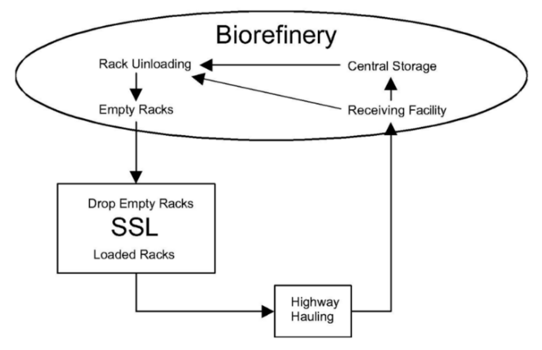
Example calculations are shown for the 0.5 bale/min biorefinery to show how the logistics system specifications were developed. Equivalent procedures were used to develop the specifications for the 1.0 and 1.5 bale/min biorefineries (programs can be accessed in the Supplementary Materials for the details analysis). The operational process is shown in Figure 1.

6.1. Total Racks and Trailers Required for 0.5 Bale/Min Biorefinery

Extra trailers are needed for each truck. At minimum, there will be a tandem unit hooked to each truck tractor and a tandem unit being loaded at each SSL where load-out operations are proceeding. The minimum number of trailers is:

5 truck tractors + 4 SSL load-outs = 9 tandem trailer sets = 18 individual trailers

At any given moment, there are racks in central storage (filled and empty) and racks on trailers (filled and empty). To determine the maximum racks required, a point of reference is chosen, and the number is calculated at that moment. The moment chosen is 1800 h Saturday when hauling operations end for the week. If a full 3 days of inventory are available at this moment, then the total filled racks are:

3 day (24 h/d) (1.5 racks/h) = 108 racks

Suppose that all trailers are parked at the plant with filled racks at 1800 h Saturday. The number of full racks in central storage is 108-9 trailer sets (2 racks/set) = 90 filled racks in storage.

There will always have to be a reserve (racks being repaired or extra empty racks), and we assign the reserve to be 5% of the total. The reserve is (108)(0.05) = 5.4~6 racks. The total number of racks required is estimated as follows (central storage + on trailers + reserve):

Total = 90 + 18 + 6 = 114 racks

The total racks processed for 48 weeks of annual operation is:

1.5 racks/h (24 h/d) (7 d/wk) (48 wk/y) = 12,096 racks/y

Average number of annual cycles for each rack in active service at any given time is:

12,096/108 = 112 cycles/y

This means that, on average, each rack is filled and emptied 112/48 = 2.33 times each week over 48 weeks of operation. This use is lower than might be expected because of the requirement to have a total of 108 full racks in storage at 1800 h on Saturday when receiving facility operations are concluded for the week.

6.2. Forklift Operation at Biorefinery

This analysis begins with one 16-Mg forklift for the 0.5 bale/min biorefinery. Productivity is not the issue; this forklift can readily unload 21 trucks (42 racks) in a 12 h haul day and simultaneously place racks in a rack unloader to maintain a continuous supply of bales for 24/7 operation. Suppose this forklift breaks down—all operations stop.

The analysis specifies two forklifts, identified as a “workhorse” and “backup”. In the case of the 0.5 bale/min biorefinery, the workhorse operator has to be on duty 24/7, 48 wk/y, or 8064 h/y. The backup operator is assumed to be available as a part-time operator with other duties associated with receiving facility operations. We assume this operator will average 6 h/d for a 6-d haul week, or 1728 h/y charged to forklift operations (

Table 5. Logistics system specifications for different capacity biorefineries.

Biorefinery (Bale/min)	Average Truckloads/d	Central Storage (m2)	Workhorse Forklift (h/y)	Backup-1 Forklift (h/y)	Backup-2 Forklift (h/y)
0.5	21	21,000	8064	1728	-
1.0	42	33,600	8064	3456	-
1.5	63	46,200	8064	5472	1728

).

The 1.0 bale/min biorefinery has a continuous operation workhorse forklift, and the backup operates 12 h/d for the 6-d haul week, or 3456 h/y, to assist with truck unloading. Nighttime operation is handled by the workhorse alone.

The 1.5 bale/min biorefinery has two continuous operation forklifts (workhorse and backup-1). A backup-2 forklift averages 6 h/d for the 6-d haul week, to assist with truck unloading and be available if one of the other forklifts is out of service. Annual operation of the backup-2 is 1728 h/y.

The forklift operating plan was selected to minimize potential delays in truck unloading. Increases in USD/Mg forklift cost is cost effective compared to an increase in USD/Mg truck cost due to increased unload time and thus lower truck productivity.

6.3. Operations Area and Central Storage at the Biorefinery

Maximum racks in central storage for a 3-day supply is 90 racks. Racks will be stacked two high; thus, there are 45, 2-rack storage spaces. Operations area for truck unloading and tandem trailer parking is needed. Total area of graded and graveled surface, allowing for needed operating area, is estimated to be 21,000 m² (2.10 ha) for a 0.5 bale/min baseline biorefinery. The entire area must be lighted for nighttime operation. For the other biorefineries, the central storage will be 33,600 and 46,200 m² for the 1.0 and 1.5 bales/min biorefinery (Table 5), respectively.

6.4. Summary of Specifications for the Different Capacity Biorefineries

The specifications for operation of the three biorefineries are summarized in Table 5, and equipment specifications are given in

Table 6. Equipment specifications for different capacity biorefineries.

Biorefinery (Bale/min)	Number Load-Outs	Number Racks	Number Trailers	Number Trucks
0.5	4	114	18	5
1.0	7	227	36	11
1.5	11	340	52	15

.

7. Cost of Feedstock Delivery for 0.5 Bale/min Biorefinery

All costs are reported USD/Mg of biorefinery annual capacity. For a biorefinery averaging 0.5 bale/min, processing bales averaging 0.4 Mg/bale, 24/7 operation, 48 wk/y, the design capacity is (0.4)(30)(24)(7)(48) = 96,768 Mg/y or 288 Mg/d. In like manner, the capacity of the 1.0 bale/min biorefinery is 193,536 Mg/y or 576 Mg/d, and the capacity of a 1.5 bale/min plant is 290,304 Mg/y or 864 Mg/d. Costs are computed using the 0.5 bale/min biorefinery as a baseline example.

7.1. Cost of Racks

The cost to own and maintain the racks is given in Appendix A. Cost on a USD/Mg basis is:

$$\frac{\mathrm{286,275} \mathrm{USD}/\mathrm{y}}{\mathrm{96,768} \mathrm{Mg}/\mathrm{y}}=2.96 \mathrm{USD}/\mathrm{Mg}$$

7.2. Cost of Trailers

The cost to own and operate the trailers (USD/d) is given in Appendix B. Using the minimum number of trailer sets, the cost, on a USD/Mg basis, is:

$$\frac{\mathrm{34,586}\frac{\mathrm{USD}}{\mathrm{y}}\mathrm{per} \mathrm{trailer} \mathrm{set} \left(9 \mathrm{trailer} \mathrm{sets}\right)}{\mathrm{96,768} \mathrm{Mg}/\mathrm{y}}=3.22 \mathrm{USD}/\mathrm{Mg}$$

7.3. Cost of SSL Load-Out Operations

At this point, the bale loader is a hypothesized machine. To calculate an ownership and operating cost, the cost and operating parameters for a “piggy-back” forklift was used, as this machine has many of the features required for a bale loader. Grisso et al. [3] estimated the cost to operate a telehandler as 41.55 USD/h and the cost to operate a bale loader as 10.32 USD/h. These costs included a labor cost for one operator and annual use of 2880 h.

For this analysis, we separate the labor cost from the cost per hour to operate the equipment (ownership + operating). A reasonable estimate of the equipment operating hours for a single SSL load-out is taken to be the total annual operating hours times the achieved productivity factor. In this case, the annual equipment operating hours are 2880 (0.525) = 1512 h (Calculated in Section 5). Equipment cost (procedures equivalent to Appendix D) on a USD/Mg basis is:

$$\frac{\left[ 18.01 \left(\mathrm{telehandler}\right)+11.18 (\mathrm{bale} \mathrm{loader}\right)]\frac{\mathrm{USD}}{\mathrm{h}} \left(1512\frac{\mathrm{h}}{\mathrm{y}}\right)\left(4 \mathrm{SSLs}\right)}{\mathrm{96,768} \mathrm{Mg}/\mathrm{y}}=1.83 \mathrm{USD}/\mathrm{Mg}$$

Labor is paid for the full 10-h day, 6 d/wk, and 48 wk/y. Benefits for the operator are estimated to be 25% of the base labor cost. The base labor cost is 25 USD/h; thus, the total labor cost is 25 × (1 + 0.25) = 31.25 USD/h. Using this cost, the average labor cost allocated to a single load-out operation, on a USD/Mg basis, is:

$$\frac{31.25\frac{\mathrm{USD}}{\mathrm{h}}\left(10\frac{\mathrm{h}}{\mathrm{d}}\right)\left(6\frac{\mathrm{d}}{\mathrm{wk}}\right)\left(48\frac{\mathrm{wk}}{\mathrm{y}}\right)\left(4 \mathrm{SSLs}\right)}{\mathrm{96,768} \mathrm{Mg}/\mathrm{y}}=3.72 \mathrm{USD}/\mathrm{Mg}$$

Cost of a service truck to support the 4 SSL load-outs was estimated as follows. Ownership + operating (no labor) cost is 1.85 USD/km. For an annual use of 61,007 km (Table 4), the annual cost is 112,863 USD/y. Labor cost for a service technician is 20 (base) × (1 + 0.25) (benefits) = 25 USD/h (2880 h/y) = 72,000 USD/y. On a USD/Mg basis, the cost is:

$$\frac{\mathrm{112,863}\frac{\mathrm{USD}}{\mathrm{y}}\left(\mathrm{truck}\right)+\mathrm{72,000}\frac{\mathrm{USD}}{\mathrm{y}}\left(\mathrm{technician}\right)}{\mathrm{96,768}\frac{\mathrm{Mg}}{\mathrm{y}}}=1.91 \mathrm{USD}/\mathrm{Mg}$$

Cost of an equipment hauler to move the telehandler and bale loader between SSLs is calculated as follows. Total cost to move the SSL load-out operations for 150 SSLs is 18,244 km (Table 4) × 3.10 USD/km (operator labor cost included) = 56,557 USD/y.

$$\frac{\mathrm{56,556} \mathrm{USD}/\mathrm{y}}{\mathrm{96,768} \mathrm{Mg}/\mathrm{y}}=0.58 \mathrm{USD}/\mathrm{Mg}$$

Total cost for the load-out operations to deliver from 150 SSLs is:

$$\left[\left(1.83+3.72\right)\left(\mathrm{SSL} \mathrm{operations}\right)+1.91 \left(\mathrm{service} \mathrm{truck}\right)+0.58 \left(\mathrm{equipment} \mathrm{hauler}\right)\right]=8.04 \mathrm{USD}/\mathrm{Mg}$$

7.4. Cost of Trucks

The truck cost is calculated based on a business plan where a trucking company supplies (for this case) five truck tractors for operations 6 d/wk, 48 wk/y. All issues associated with ownership and operation of the trucks is included in the contract. The feedstock manager at the biorefinery can send any truck to any SSL where a load is ready. For this analysis, there is no attempt to ensure that all trucks obtain approximately the same haul distance assigned for a given day. Variability in haul distance might typically be handled with a mass-distance fee. For example, a 16 Mg load hauled 30 km would be a 16 × 30 = 480 Mg-km haul. If this truck hauls four loads/d, the total is 4 × 480 = 1920 Mg-km. A second truck might be assigned a 15 km haul, and it hauls six loads/d. The mass-distance parameter 6 × 16 × 15 = 1440 Mg-km. A Mg-km fee in the hauling contract might be developed as the feedstock logistics system matures. The analysis here envisions that the biorefinery will contract for five trucks, and it is the responsibility of the biorefinery to deploy these trucks to achieve the highest possible productivity (Mg/d) for the truck fleet.

The business plan specifies that fuel will be supplied by the biorefinery. For this reason, fuel cost is calculated separately.

Rental cost for a single-axle, pintle hitch truck tractor (Penske Truck Rental) is 845 USD/wk. Annual cost for a single truck tractor is:

$$845\frac{\mathrm{USD}}{\mathrm{d}} \left(48\frac{\mathrm{wk}}{\mathrm{y}}\right)=\mathrm{40,560}\frac{\mathrm{USD}}{\mathrm{y}}$$

The total haul distance is 561,834 km (Table 3); therefore, each of the five trucks averages 112,367 km. If a truck averages 1.7 km/L fuel (fuel cost of 0.79 USD/L), annual fuel cost is 52,218 USD.

Labor cost for an operator is 25 (base) (1 + 0.25) (benefits) = 31.25 USD/h. For 12 h haul day, 6 d/wk, and 48 wk/y, the annual labor cost is 108,000 USD/y. Insurance cost is based on a well-run trucking company doing short-haul operations in Central Virginia. (No reference is given because the insurance company does not want the cost estimate to be considered a quote.) Total truck cost is 40,560 (rental cost) + 8500 (insurance) + 52,218 (fuel) + 108,000 (labor) = 209,278 USD/y.

Cost of the truck tractors on a USD/Mg basis is:

$$\frac{\mathrm{209,278} \frac{\mathrm{USD}}{\mathrm{y}}\left(\mathrm{per} \mathrm{truck}\right) \left(5 \mathrm{trucks}\right)}{\mathrm{96,768}\frac{\mathrm{Mg}}{\mathrm{y}}}=10.82 \mathrm{USD}/\mathrm{Mg}$$

7.5. Cost of Biorefinery Storage and Operating Area

The cost to own and operate a 2.10 ha gravel storage yard with needed lighting for nighttime operation is given in Appendix C. Cost (USD/Mg) is:

$$\frac{\mathrm{89,912} \mathrm{USD}/\mathrm{y}}{\mathrm{96,768} \mathrm{Mg}/\mathrm{y}}=0.93 \mathrm{USD}/\mathrm{Mg}$$

7.6. Cost of 16-Mg Forklifts at the Receiving Facility

Estimated weight of a loaded rack is 10.5 Mg; thus, a 16 Mg forklift is specified. The workhorse forklift operates 24/7, 48 wk/y. Equipment operating cost (Appendix D) is estimated at 22.75 USD/h. Cost (USD/Mg) is:

$$\frac{22.75\frac{\mathrm{USD}}{\mathrm{h}}\left(24\frac{\mathrm{h}}{\mathrm{d}}\right)\left(7\frac{\mathrm{d}}{\mathrm{wk}}\right)\left(48\frac{\mathrm{wk}}{\mathrm{y}}\right)}{\mathrm{96,768} \mathrm{Mg}/\mathrm{y}}=1.90 \mathrm{USD}/\mathrm{Mg}$$

Using a labor cost of 31.25 USD/h, including benefits, the USD/Mg labor cost assigned to the workhorse forklift is 2.61 USD/Mg.

The backup forklift is expected to operate about 50% of the 12 h receiving facility workday, 6d/wk, 48 wk/y. The calculations shown in Appendix D were conducted for an annual operation of 1728 h, and cost was 26.42 USD/h or 0.47 USD/Mg. The labor cost associated with operation of the backup forklift is 0.56 USD/Mg.

Total cost to operate the two 16-Mg forklifts is (1.90+2.61+0.47+0.56) = 5.54 USD/Mg.

8. Discussion

The average cost to deliver feedstock to the biorefinery for year-round operation is given in

Table 7. Cost of unit operations for different capacity biorefineries (USD/Mg annual capacity).

Biorefinery (Bale/min)	SSL Load-Outs	Racks	Trailers	Trucks	Receiving Storage	Facility Forklifts	Total
0.5	8.04	2.96	3.22	10.82	0.93	5.54	31.51
1.0	6.47	2.95	3.22	11.63	0.91	3.24	28.42
1.5	6.32	2.94	3.10	10.81	0.75	3.00	26.92

. The cost computation begins with feedstock in the SSLs and ends when a rack is placed in the rack unloader at the biorefinery.

There is some modest “economy of scale” influence shown in Table 7. The operating area required at the biorefinery receiving facility is only a little smaller for the 0.5 bale/min as compared to the 1.5 bale/min biorefinery. The area to store the racks is smaller for the 0.5 biorefinery, but when the two requirements are added, the reduction in total area does not decrease linearly. Of more significance is the 16 Mg forklift cost. Two forklifts are required for both the 0.5 and 1.0 bale/min biorefineries. These two machines are not utilized to their full potential for the 0.5 bale/min biorefinery, thus the higher USD/Mg cost. Three 16-Mg forklifts are specified for the 1.5-bale/min biorefinery. Recapping their annual operating hours, the workhorse operates 8064 h/y, backup-1 operates 5472 h/y, and backup-2 operates 1728 h/y (Table 5). These operating assumptions are believed to be conservative.

There is a 14.6% decrease in average delivered cost for a three-fold increase in biorefinery capacity. This rather encouraging result is tempered by considering the constraint that all feedstock is produced within a 50 km radius. The percentage of total land area within this radius attracted into feedstock production increases for 1.8 to 5.5%. If feedstock density (Mg/km²) had been held constant as refinery capacity increased, then average haul distance would have increased, and total delivered cost would increase.

The following discussion focuses on the 1.0 bale/min processing rate for the biorefinery. Cost of the trucks is 41% of the total, load-out operations are 23%, and racks plus trailers is 22%. As expected, truck cost is the largest component of the delivery cost. Truck cycle time is minimized for this analysis. The only viable method for reducing truck cost is to increase truck productivity (more Mg hauled per day per truck), and the only viable way of achieving this goal is to increase loads/d. This requirement strongly advocates for central control. Technology is available to know in real-time the location of every truck and the status of every load-out operation. This technology is used commercially by other industries. It will be used by a mature biorefinery industry to achieve the most cost-effective highway hauling.

The labor productivities of the worker at an SSL load-out and the truck driver are compared in

Table 8. Labor productivity of load-out operator and truck operator.

Biorefinery Capacity (Bale/min)	Load-Out Productivity (%) (Mg/h)		Truck Productivity (%) (Mg/h)
0.5	52.5	8.4	61.2	5.6
1.0	60.0	9.6	55.7	5.1
1.5	57.3	9.2	61.0	5.6

. Productivity (Mg/h) of the load-out operator ranges from 1.5 to 1.9 times that of the truck driver. This result is explained by the cycle time for the truck; travel speeds and distances set the time to move a given mass. Increasing loads per day is the only viable option to increase truck driver labor productivity, and central control is needed to achieve this increase.

The authors argue that, with the correct business plan, implemented with the correct information systems technology (central control), a truck productivity of 50–60%, used for this analysis, can be increased to 70%. A cost analysis was performed for a truck fleet with one less truck and a fleet with one additional truck. The same total haul distance was used for all three truck fleets. As shown in

Table 9. Influence of truck productivity on cost (USD/Mg annual capacity).

Biorefinery Capacity (Bale/min)	Truck Productivity (%)	No. Trucks	Truck Cost (USD/Mg)
0.5	76.5	4	9.19
	61.2	5	10.83
	51.0	6	12.44
1.0	61.2	10	10.85
	55.7	11	11.63
	51.0	12	12.45
1.5	65.0	14	10.27
	61.0	15	10.81
	57.0	16	11.35

, the truck cost increases about 3.25 USD/Mg as the truck fleet for the 0.5 bale/min biorefinery increases from four to six trucks. For the 1.0 bale/min biorefinery, the cost increase is 1.60 USD/Mg as the truck fleet is increased from 10 to 12 trucks. Increasing the fleet from 14 to 16 trucks gave an increase of 1.08 USD/Mg for the 1.5 bale/min biorefinery.

The rack system, because it minimizes load time and unload time, does provide a method to increase truck productivity. We argue that this investment is cost effective, and it should be the central element of the feedstock delivery system.

9. Conclusions

Hauling by the biorefinery provides an opportunity for small- and intermediate-size farmers to participate in a biorefinery supply chain. Central control of hauling, where a feedstock manager can set the order of SSLs being unloaded and send a truck to any SSL with a load waiting, can maximize both load-out and truck productivity (Mg/d). The rack system solves the problem of safe and efficient hauling of round bales. Of equal or perhaps greater importance, it solves the problem of single-bale handling at the biorefinery. All handling for 24/7 operation, placement into central storage and removal from storage, is conducted with the 20-bale rack.

A key question is the cost of the racks and required support equipment to fill, transport, and unload racks. A 2-trailer tandem pulled by a truck tractor is a truckload (40 bales). Truck load time at the SSL is minimized by dropping a tandem trailer set with empty racks and towing a waiting full set. This requires, at minimum, that each truck is towing a set, and one set is parked at each SSL load-out. The analysis specifies that all central storage be bales-in-racks, and the maximum storage is a 3-day supply at full biorefinery capacity. The analysis shows that rack cost to supply a biorefinery processing a 1.0 bale/min for 24/7 operation is ~3.00 USD/Mg of annual biorefinery capacity, and the rack trailer cost is ~3.20 USD/Mg. Total delivery cost, beginning with bales in SSL storage and ending with a rack being placed in an unloader to deliver individual bales for processing, is 31.51, 28.42, and 26.92 USD/Mg for a biorefinery processing 0.5, 1.0, and 1.5 bale/min, respectively.

References

- Judd, J.D.; Sarin, S.C.; Cundiff, J.S. Design, modeling, and analysis of a feedstock logistics system. Bioresour. Technol. 2012, 113, 209–218. [Google Scholar] [CrossRef] [PubMed]
- Grisso, R.D.; Cundiff, J.S.; Comer, K. Multi-bale handling unit for efficient logistics. AgriEngineering 2020, 2, 336–349. [Google Scholar] [CrossRef]
- Grisso, R.D.; Cundiff, J.S.; Sarin, S.C. Rapid truck loading for efficient feedstock logistics. AgriEngineering 2021, 3, 158–167. [Google Scholar] [CrossRef]
- Cundiff, J.S.; Grisso, R.D.; Fike, J. Feedstock contract considerations for a piedmont biorefinery. AgriEngineering 2020, 2, 607–630. [Google Scholar] [CrossRef]
- Ravula, P.R.; Grisso, R.D.; Cundiff, J.S. Cotton logistics as a model for a biomass transportation system. Biomass Bioenergy 2008, 32, 314–325. [Google Scholar] [CrossRef]
- Circle, F.D. Demonstration of an Advanced Supply Chain for Lower Cost, Higher Quality Biomass Feedstock Delivery; Final Report DOE Grant Award Number DE-EE0006300; FDC Enterprises: New Albany, OH, USA, 2021. [Google Scholar]
- Aguayo, M.M.; Sarin, S.C.; Cundiff, J.S.; Comer, K.; Clark, T. A corn-stover harvest scheduling problem arising in cellulosic ethanol production. Biomass Bioenergy 2017, 107, 102–112. [Google Scholar] [CrossRef]
- USDA NASS. 2017 Census of Agriculture. 2017. Available online: https://www.nass.usda.gov/Publications/AgCensus/2017/index.php (accessed on 22 June 2021).
- Gordian. RSMeans Data from Gordian; Construction Publishers & Consultants: Rockland, MA, USA, 2021; Available online: https://www.rsmeans.com/ (accessed on 22 June 2021).
Figure 1.
Operation sequence and order of the load and unload technology.