Stress Detection Using Proximal Sensing of Chlorophyll Fluorescence on the Canopy Level

Abstract

Chlorophyll fluorescence is interesting for phenotyping applications as it is rich in biological information and can be measured remotely and non-destructively. There are several techniques for measuring and analysing this signal. However, the standard methods use rather extreme conditions, e.g., saturating light and dark adaption, which are difficult to accommodate in the field or in a greenhouse and, hence, limit their use for high-throughput phenotyping. In this article, we use a different approach, extracting plant health information from the dynamics of the chlorophyll fluorescence induced by a weak light excitation and no dark adaption, to classify plants as healthy or unhealthy. To evaluate the method, we scanned over a number of species (lettuce, lemon balm, tomato, basil, and strawberries) exposed to either abiotic stress (drought and salt) or biotic stress factors (root infection using Pythium ultimum and leaf infection using Powdery mildew Podosphaera aphanis). Our conclusions are that, for abiotic stress, the proposed method was very successful, while, for powdery mildew, a method with spatial resolution would be desirable due to the nature of the infection, i.e., point-wise spread. Pythium infection on the roots is not visually detectable in the same way as powdery mildew; however, it affects the whole plant, making the method an interesting option for Pythium detection. However, further research is necessary to determine the limit of infection needed to detect the stress with the proposed method.

1. Introduction

Modern advanced greenhouses are increasingly equipped with control functionalities. The temperature, humidity, CO₂-concentration, and light intensity can be controlled to optimal values, and irrigation and fertilization can be automated [1]. An interesting development for automated and efficient precision agriculture is the detection and diagnosis of plant stress. Standard methods for stress detection are often destructive or disruptive [2] and, hence, not an option for on-line detection.

However, much research has been carried out in the area of optical sensors [3] for measuring the reflected and fluorescent light from the canopy as a mean for non-distruptive remote sensing of stress. Even though many methods have been suggested, sensor-based phenotyping is still at an early stage of development and not yet commonly applied in the field [3,4]. Thus, there is still a need for more research to develop reliable and cost-effective sensors for stress detection [2].

The light energy absorbed by the plants is used for photosynthesis, reemitted as heat, or reemitted as fluorescence. This has made fluorescence an indispensable tool for studying photosynthesis in a wide range of applications [5,6]. In particular, if stress factors influence the plants in a way such that the photosynthesis is affected, one would expect an influence on the fluorescence response as well.

Fluorescence is classically measured and analysed using a pulse amplitude modulation fluorometer (PAM) and requires measurements from both fully dark adapted plants and plants at fully saturating light [7]. In practice, this restricts its use to mainly on-leaf measurements. Another, completely different, fluorescence based method is sensing of solar induced fluorescence (SIF) [8,9]. This is a passive method, done remotely on an airborne scale, measuring the fluorescence of a whole field, for example.

In between remotely sensed and on-leaf level sensed fluorescence, there is proximal sensing [10]. One method using proximal sensing of fluorescence is the laser induced fluorescence transient (LIFT) technique [11]. A blue laser projects a collimated beam onto the leaves, in flashlets of 1.6 μs and in excitation protocols with up to 7500 flashlets [12]. The emitted fluorescence at 690 nm is collected and then used to determine the photosynthetic properties. The LIFT device can be used both in labs and in the field, at distances up to 50 m [13]. Another innovation in the field of proximal sensing and fluorescence measurements, was presented by Urschel and Pocock [14]. It uses a chlorophyll a fluorometer, developed to capture canopy level red and far-red fluorescence (i.e., the peaks around 685 and 740 nm), induced by saturating light pulses. The instrument, however, was mainly developed to monitor growth.

There is a great deal of ongoing research on advanced optical sensors for stress detection (see review articles [2,4,15]). A wide range of spectral and spatial resolutions on the sensors are used; fluorescence spectroscopy [16,17] and multicolour fluorescence imaging [18] as well as hyperspectral imaging [19,20,21,22]. Such equipment generates large amounts of data, and one method of handling these data is to use machine learning algorithms for feature selection [21] as well as for classification. For a review of classification of biotic stresses using machine learning, please see [23].

Not only are different types of sensors under investigation but also many different types of light protocols are used when gathering data. In addition to referring to the reviews, we highlight a few recent and, from our point of view, particularly interesting studies: Sun et al. [24] investigated three different mutants of Arabidopsis and their resistance to drought stress. Kinetic chlorophyll fluorescence imaging data was collected at a distance between the sample and the lens of about 20 cm. The plants were subjected to dark adaption for 15 min, followed by a measurement sequence of 200 s, where the light protocol consisted of several saturating light pulses in a dark background or in a constant actinic background light.

Deep learning methods were applied to extract features, which were then used as inputs for a machine learning classification algorithm. Blumenthal et al. [25] used video imaging data from a prototype set-up (GrowScanner, GrowTech Inc., Lexington, MA, USA). Their process starts with dark adaption, followed by light excitation and measurements of the fluorescence intensity on one point of the leaf during 15 s. The smoothed intensity signal, as well as its derivative, are used as inputs to an unsupervised machine learning algorithm (Hidden Markov Models), to cluster plants with respect to the type of stress and stress level.

Römer et al. [17] used a compact fiber-optic fluorescence spectrometer with a laser as the excitation source, placed a few millimetres from the leaf and measuring the spectrum with a resolution of 2 nm in the range 370–800 nm. To reduce the numbers of features, piecewise polynomials were fitted to the data and a (Support Vector Machine) classifier could then, with a high accuracy, distinguish between healthy and unhealthy wheat leaves.

All though showing promising results, all the methods above rely on saturating light and/or dark adaption, which are difficult to accommodate in the field or in a greenhouse. The measurements used for stress detection in this study are based on the dynamic fluorescence response (DFR), i.e., dynamic characteristics of the fluorescence response to weak and long light excitation pulse, without prior dark adaption. A spectrometer was used to measure the fluorescence at the canopy level, i.e., through proximal sensing of fluorescence.

We have previously shown correlation with photosynthesis [26,27,28] and used it for growth tracking [29] and for light stress detection [30,31,32]. In the latter work, the variations in the DFR originating from a weak excitation from a blue LED light were used for light stress detection. The dynamics in the response in the fluorescence signal on a minute-scale could be used to distinguish between different light stress levels.

We hypothesized that it is possible to distinguish between healthy and various kinds of abiotically or biotically stressed plants, by analysing the information in the fluorescence signal. We investigated this by using a method similar to the DFR-method and extracted features from the dynamic responses to be used in a machine learning classification context.

Several stress factors were scanned: drought (lettuce) and salt stress (lettuce and lemon balm), root infection with the fungal pathogen Pythium ultimum (basil, tomato, and lettuce), and infection with the fungal pathogen for Powdery mildew, Podosphaera aphanis (strawberries). The strengths of this method are that the measurements are done on-line, remotely on the canopy level, and that the plants neither need to be dark adapted nor exposed to saturating light.

Furthermore, market available LED lamps were used in the experiments, and the blue channel was used to construct the weak excitation signal in the form of a positive step change. For this study, a spectrometer was used but a simpler, cheaper type of photodiode with a bandpass optical filter could be applicable. In such a case, it could be economically justified to distribute sensors over entire greenhouses.

2. Materials and Methods

A variety of different plant species and stress factors were investigated in this screening study where proximal fluorescence step response measurements were made on one or multiple plants at a time.

2.1. Plant Materials and Cultivation Conditions

The abiotic stress experiments were conducted at the Heliospectra PlantLab in Gothenburg, while the biotic stress experiments were conducted at the Swedish University of Agricultural Sciences (SLU), Alnarp, Sweden. All experimental setups included both healthy reference plants and plants exposed to stress factors.

2.1.1. Abiotic Stress

The abiotic stress factors investigated were salt and drought stress. All these tests were performed in an indoor growing facility where the light, temperature, and humidity were controlled (200 ± 20 μmol m⁻² s⁻¹, 22/16 °C day/night temperature, and RH 60%). Two cultivars of lettuce (Lactuca sativa cv. Great lakes 118, referred to as lettuce ‘a’, and another cultivar from a commercial grower in Sweden, referred to as lettuce ‘b’) were used for measurements for both stress factors. The measurements were conducted around 4 weeks after sowing.

For salt stress, additional measurements were made on a third cultivar of lettuce (Batavia lettuce cv. Othilie^RZ, referred to as lettuce ‘c’) and lemon balm (from a commercial grower in Sweden). Those measurements were conducted 4–6 weeks after sowing. The plants were grown in a mix of two parts of soil and one part of vermiculite. The sample sizes were seven pots of each lettuce ‘a’ and ‘b’ (two salted, two dried, and three reference), 20 pots of lettuce ‘c’ (nine salted and 11 reference) and 14 pots of lemon balm (eight salted and six reference). The total number of measurements conducted were 23 for lettuce ‘a’ (15/4/4 on ref/salt/dry), 31 for lettuce ‘b’ (15/8/8 for ref/salt/dry), 27 for lettuce ‘c’ (15/12 for ref/salt), and 26 for lemon balm (16/10 on ref/salt).

The plants in the reference group were watered every morning. For the salt-stressed group, the daily watering was replaced by watering with salty water (200 mM NaCl), starting the day before the first measurement. Hence, they were assumed to become increasingly stressed over time. The plants in the drought stress group received no water one day before the first measurement and were further only occasionally watered with a lesser amount of water. This was to avoid wilting within the week that the measurements were collected. The moisture content in the soil was monitored as a reference of the drought level.

2.1.2. Biotic Stress

Root infection with Pythium ultimum

Six pots of each species; basil (Ocimum basilicum cv. Basilikum), tomato (Solanum lycopersicum cv. Picolino), lettuce ‘a’ and ‘b’ (see Section 2.1.1) were planted for the experiment with the root pathogen Pythium ultimum. Unfortunately, one tomato did not grow, hence, one sample less of that species was available. The plants were grown in a greenhouse in Alnarp, Sweden, during sunny days in June 2020. No supplemental light was used, and the RH was 80%. The temperature varied over the day and peaked above 30 °C.

An inoculum of Pythium was prepared as described by Hultberg et al. [33]. Briefly, mycelium from Pythium grown on PDA (Difco 213400) were transferred to and grown on water agar plates for two days. Small pieces (1 × 1 cm) were then cut from the periphery of the colony and transferred to a Petri dish with 15 mL of cleared fruit juice broth (11.5 g of rolled oats boiled with 125 mL of V8 fruit juice (Friggs, Sweden) and 500 mL water). The suspension was centrifuged for 15 min at 500 g (Avanti J-20, Beckman Coulter, CA, USA).

The supernatant was diluted with water to 625 mL, 0.94 g of CaCO₂ was added, and the broth was autoclaved. The Petri dishes were incubated in darkness for three days at 25 °C. The mycelium was washed twice in an autoclaved mineral solution (0.145 g Ca(NO₃)₂, 0.012 g MgSO₄, 0.099 g KH₂PO₄, and 0.016 g FeCl₃, L⁻¹) and once in autoclaved distilled water.

The mycelium was then transferred to Petri dishes with 15 mL of autoclaved distilled water, incubated at 40 °C for 30 min and then transferred to room temperature. The zoospores were released after about 1 h. The zoospore suspension was carefully collected in sterile vessels, and zoospores were counted in a haemocytometer.

The fungus was grown for 3 weeks at 22 °C in 20 mL of Schmitthenner’s medium. The mycelium was briefly homogenized in a blender and diluted with NaCl to $3\times 103$ CFU ${\mathrm{mL}}^{-1}$ (Colony forming units) as enumerated on PDA (Potato Dextrose Agar) media containing 200 mg ${\mathrm{L}}^{-1}$ kanamycin. The Pythium suspension was added to the sowing soil/substrate three times: at 3, 4, and 5 weeks after sowing. Every week, two to five measurements were conducted on each plant species and each group (ref/infected).

Leaf infection with Podosphaera aphanis

For the experiment with the leaf pathogen of Powdery mildew, Podosphaera aphanis, strawberry cuttings were planted in pots and grown in the greenhouse. Out of the 90 plants, 1/3 were moved to another cultivation chamber in the greenhouse where they were infected with powdery mildew. The infection was done with help of other heavily infected plants that were placed among the plants to be infected and, with a brush, the spores were moved to those plants. This was done daily throughout the whole experiment.

Four days after infection, all plants were moved into a growth chamber, with one room for the infected plants and one identical room for the reference plants. This is referred to as day 1 (week 1) of the experiment, from which the measurements started and continued for one month. The light intensity was 300 μmol m⁻² s⁻¹ (8:00 a.m.–10:00 p.m.), and the temperature was 22 °C. The RH was initially 60%; however, from day 3, it was increased to 70% (and 85% at 2:00 p.m.–6:00 p.m.). The increased humidity was to enhance the spread of pathogen.

The experimental unit, in which the fluorescence step response measurements were conducted, was placed in the room of the infected plants. To reduce the risk of spread of the pathogen into the room with healthy plants, no plants were moved back there. Thus, the healthy plants were consumed as reference once they had been subjected to measurements, this being the reason for starting with 2/3 of the plants in the healthy group.

2.2. Experimental Setup

Here, we present information about the experimental unit, i.e., the box mounted with lamps and spectrometers to which the plants were moved for measurements, as well as the light scheme used to extract information in the fluorescence signal. The data preparation of the fluorescence signal and the used reference measurements are also described.

2.2.1. Experimental Unit

As the abiotic and biotic stress experiments were conducted at different locations (Gothenburg and Alnarp, Sweden), two different experimental units were used. The only thing that differed between them was the dimensions of the units, 2 × 1 × 1 m (H × W × D) in Gothenburg and 2 m × 1 m × 0.8 m in Alnarp. The units consist of aluminium profiles that hold white, highly diffusive, and reflective walls in place. At the top, three Heliospectra LX lamps are mounted; two for background light and one for excitation light, all placed about 1.5 m above the plants.

A spectrometer (STS, Ocean Insight, Orlando, FL, USA) was placed on the canopy level, facing the lamps, to measure the incident light with an integration time of 0.1–0.2 s, depending on the light intensity. A second spectrometer (QE65000, Ocean Insight, Orlando, FL, USA) was equipped with a 600 μm optical fibre, placed in between the lamps, and pointing downwards, thus, measuring the reflected and fluorescent light from the plants. As the fluorescence signal is relatively weak, the integration time was long (normally 0.8 s, in a few abiotic stress experiments even 1–2 s), to obtain a stable signal. The lamps and the spectrometers were controlled with a scheme programmed in MATLAB (Mathworks Inc., Natick, MA, USA).

2.2.2. Light Scheme

The plants were moved one at a time (two at a time for strawberries) to the experimental unit for the fluorescence step response measurements without any dark adaption. The lamps first hold the (lowest) background light for a few minutes for the plants to adapt to the new light level. When the light scheme starts, it keeps the background light level for another 4–5 min, whereafter a blue constant excitation light (30–70 μmol m⁻² s⁻¹) is added over 3 min. This is sequentially repeated for several background light levels. An example is shown in Figure 1, where (a) is the incident light within the PAR region (400–700 nm) and (b) is the fluorescence, integrated over the wavelengths 720–760 nm.

An overview of all settings for the different experiments is presented in

Table 1. The settings for all experimental sets.

	Abiotic Stress		Biotic Stress
Stressor	Salt & Drought	Salt	Pythium	Powdery Mildew
Crop species	Lettuce ‘a’,	Lettuce ‘c’,	(i) Lettuce ‘a’,	Strawberries
	Lettuce ‘b’	Lemon balm	Lettuce ‘b’,
			(ii) Basil, Tomato
Growing	Closed	Closed	Greenhouse	Closed *
environment
Bkg light	5 min	4 min	5 min	5 min
μmol m−2 s−1	55, 110, 135, and 200	85, 215, 465, and 760	(i) 110, 215, and 275	110, 110, 215, and 215
			(ii) 215, 275, and 405
Excitation light	3 min	3 min	3 min	3 min
μmol m−2 s−1	30	45	70	70

* The strawberries were grown in a greenhouse prior to the experiment.

. The light levels presented are the ones measured during the experiments. The variation in excitation light intensity were not intended and were only a result of different setups. Regarding the light intensity levels, we were initially interested in scanning a wide range of intensities. However, based on the results from the salt stress experiments, slightly lower light intensities were used for the remaining abiotic stress experiments.

In the Pythium setup, higher light intensities were chosen for basil and tomato, compared to for lettuce, as they were expected to handle high light better. The powdery mildew setup started with a very small pilot study where four different light levels were included (110, 215, 275, and 400 μmol m ⁻² s⁻¹), where the two lower ones looked the most promising and were, thus, chosen for the main setup.

2.2.3. Data Preparation

The light in the region 400–700 nm is considered as photosynthetically active radiation (PAR), and therefore the incident light detected by the spectrometer was integrated over this wavelength interval. This was considered as the input signal to the system. The output signal was the chlorophyll a fluorescence, ChlF, integrated over the wavelength span of 720–760 nm. The ChlF has two peaks; one at 685 nm and one at 740 nm. However, earlier research has shown a stronger correlation between photosynthesis and the fluorescence signal in the 740 nm region (compared to the 685 nm region) [27], hence, the peak choice in this setup.

To enable comparisons between sets with different background light, the data was normalized. The ChlF curves for each background light level were first shifted to an intensity equal to zero just before the excitation step started and then normalized such that the response signal was (approximately) equal to one at the end of the excitation, according to

$$y_{normalized}=(\mathrm{raw}\mathrm{data}-y_{zero})/y_{one},$$

(1)

where

$$\begin{array}{cc}\hfill y_{zero}& =\mathrm{mean}\mathrm{value}\mathrm{of}\mathrm{ChlF}\mathrm{the}\mathrm{last}1\min \mathrm{of}\mathrm{the}\mathrm{background}\mathrm{light}\mathrm{level},\mathrm{and}\hfill \\ \hfill y_{one}& =\mathrm{mean}\mathrm{value}\mathrm{of}\mathrm{ChlF}\mathrm{the}\mathrm{last}1\min \mathrm{of}\mathrm{the}\mathrm{excitation}.\hfill \end{array}$$

Two parameters that we paid extra attention to were the maximal fluorescence value during the excitation, referred to as the peak value, and the peak time, which is the time from the start of the excitation to the time the peak value occurs (Figure 2). These values were extracted from smoothed data (window width of five samples) to decrease the impact of noise.

When interested in how dispersed measurements in a sample are, we used the standard deviation (std), defined as

$$\begin{array}{c}\hfill std=\sqrt{\frac{1}{n-1}\sum _{i=1}^n{(y_i-\overline{y})}^2},\end{array}$$

(2)

where n is the number of samples, $y_i$ is measurement i and $\overline{y}$ is the mean value of the measurements. When interested in how close the sampled mean and the true population mean are to each other, the standard error of the mean, defined as

$$\begin{array}{c}\hfill sem=\frac{std}{\sqrt{n}},\end{array}$$

(3)

was considered instead.

To verify whether two parameters statistically differed from each other, for example whether the mean value $\mu$ (of the peak time, or the peak value) differed between the healthy and the stressed group, a two sampled t-test was used [34]. Then, the null hypothesis ($H_0$) and the alternative hypothesis ($H_1$) were formulated according to

$$\begin{array}{c}\hfill H_0:{\mu }_{\mathrm{healthy}}={\mu }_{\mathrm{stressed}}\\ \hfill H_1:{\mu }_{\mathrm{healthy}}\ne {\mu }_{\mathrm{stressed}}\end{array}$$

(4)

where $\mu$ was the mean value of each group.

2.2.4. Reference Measurements

Abiotic stress

In the drought stress experiment, the volumetric water content in the soil was measured with an EC-5 (METER Group Inc., Pullman, WA, USA).

In the salt stress experiment, the plants continued to receive salty water throughout the experiment, with a consequent accumulation in the total amount of salt added. Hence, days after experimental start is a measure assumed to correlate with the stress level. No other explicit measure of stress level was used.

Biotic stress

Three weeks after Pythium inoculation, the plants were harvested and separated into two parts: the root part and the part with the leaves together with the stems. These parts were subjected to dry weight measurements. The method for estimating the amount of Pythium on the roots is described in [35].

About 20 g of fresh weight roots was first macerated in a mortar for 2 min after the addition of 50 mL of detergent solution (0.1% peptone and 0.2% sodium hexametaphosphate). The mixture was then shaken at 200 rpm for 20 min at room temperature. An amount of 1 mL of the mixture was serially diluted in 9 mL NaCl, and 100 μL volumes of the serial dilution were spread, in triplicate, on PDA-plates containing 200 mg L⁻¹ of kanamycin after incubation of the plates in 25 °C for 24 h. Based on colony counting, the CFU g⁻¹ DW root was calculated.

The maximum photosynthesis ($A_{max}$) was measured at a light intensity of 1000 μmol m⁻² s⁻¹ using an infra-red gas analyser photosynthesis instrument (LCPro+, ADC Bioscientific, Hoddesdon, UK). The light was supplied using the internal LED-array with red and blue LEDs. The measured values were allowed to stabilize for 20 min before readings. The measurements were conducted on experimental day 11 (on tomato, basil, and lettuce ‘a’) and again on day 19 (on tomato and basil).

The strawberries in the powdery mildew experiment were visually inspected throughout the experiment to obtain an idea of how the mildew spread. Figure 3 shows an example of different degrees of powdery mildew infection.

3. Results

3.1. Abiotic Stress

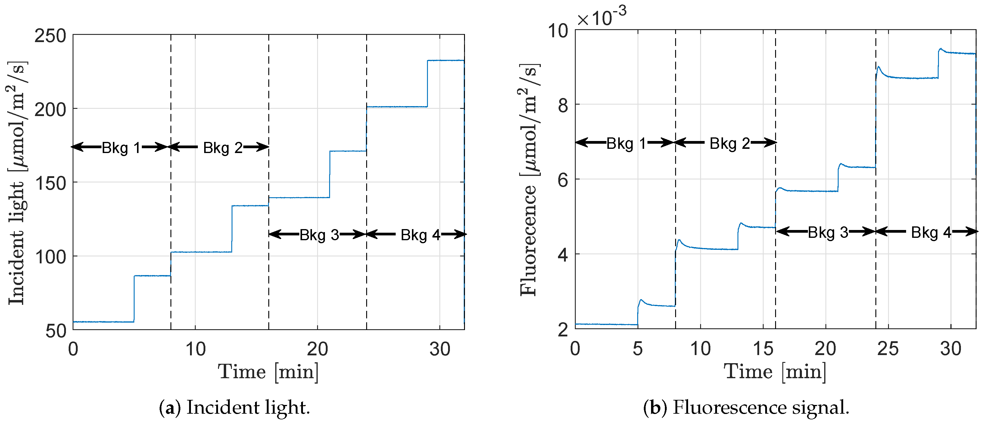
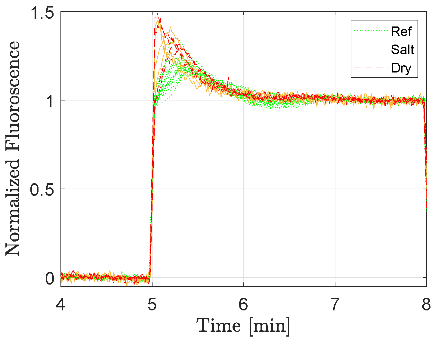
The fluorescence step response was measured on lettuce ‘a’ and ‘b’, on healthy, dry, and salt-stressed plants. Figure 4 shows all the fluorescence responses (normalized according to Equation (1)) for lettuce ‘a’ at the lowest background light level. Green dotted lines correspond to reference plants, solid orange lines are the salt-stressed plants, and the red dashed lines are the dry ones. As can be seen, the initial dynamics after the step excitation differed between the plants depending on their conditions.

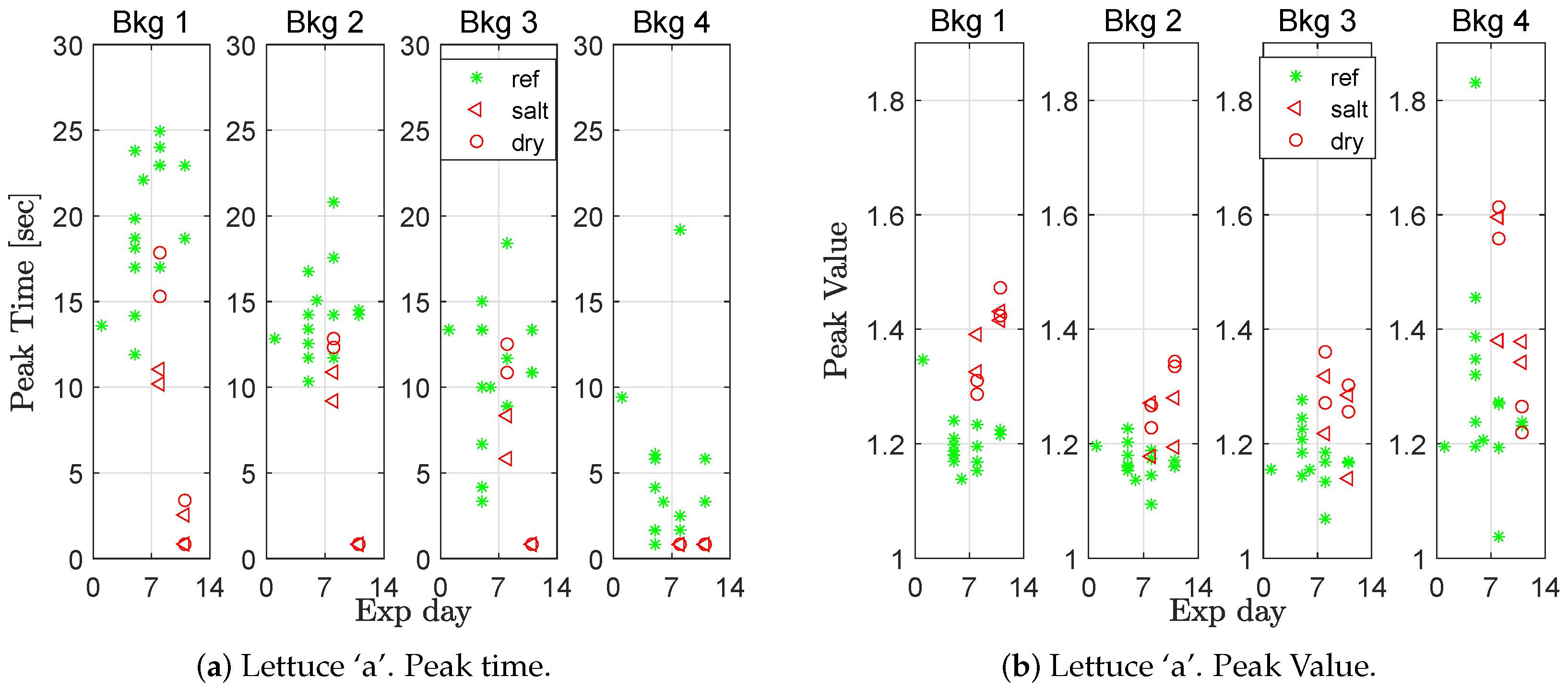
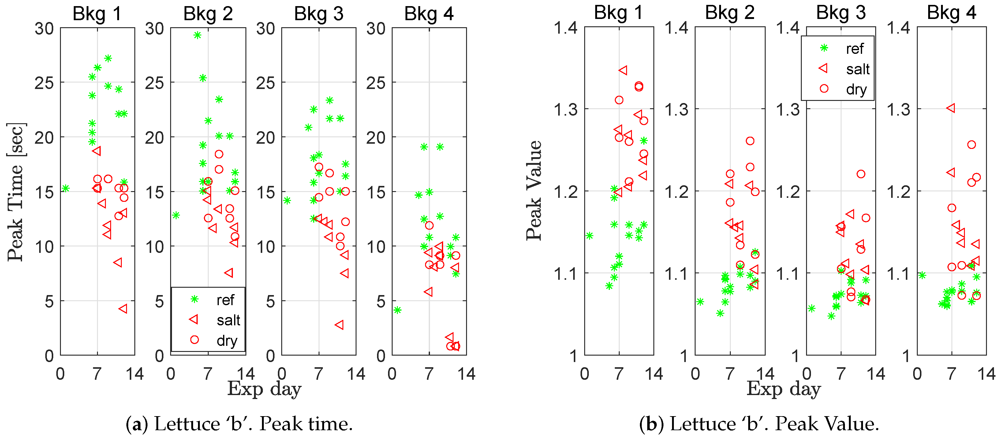
For each of the four different background light levels (ranging from 55 to 200 μmol m⁻² s⁻¹), the peak time and the peak value (for definition see Figure 2) of the responses were extracted. The results for lettuce ‘a’ are presented in Figure 5 and for lettuce ‘b’ in Figure 6. The stressed plants generally had a shorter peak time and a higher peak value. In Appendix A (

Table A1. Two way ANOVA table, comparing peak times and peak values in abiotic stress experiments. A, B, and C: lettuce ‘a’, reference, salt-, and drought-stressed plants. D, E, and F: lettuce ‘b’, reference, salt-, and drought-stressed plants.

Comparison		Bkg Light	df	tstat	sd	p	h
Group	Parameter
A and B	peak time	1	17	5.42	4.31	4.6 $\times {10}^{-5}$	1
A and B	peak time	2	17	4.78	3.27	1.8 $\times {10}^{-4}$	1
A and B	peak time	3	17	2.69	4.21	0.016	1
A and B	peak time	4	16	1.62	4.32	0.126	0
A and B	peak value	1	17	−1.85	0.05	2.8 $\times {10}^{-6}$	1
A and B	peak value	2	17	−1.95	0.04	0.009	1
A and B	peak value	3	17	−1.06	0.06	0.056	0
A and B	peak value	4	16	−1.85	0.10	0.012	1
A and C	peak time	1	17	3.44	5.15	0.003	1
A and C	peak time	2	17	3.60	3.71	0.002	1
A and C	peak time	3	17	1.53	4.72	0.144	0
A and C	peak time	4	16	1.61	4.32	0.126	0
A and C	peak value	1	17	−1.20	0.06	7.3 $\times {10}^{-5}$	1
A and C	peak value	2	17	−1.86	0.04	1.9 $\times {10}^{-5}$	1
A and C	peak value	3	17	−1.42	0.05	3.8 $\times {10}^{-4}$	1
A and C	peak value	4	16	−1.21	0.13	0.042	1
D and E	peak time	1	21	5.95	4.19	6.7 $\times {10}^{-6}$	1
D and E	peak time	2	21	3.95	3.91	7.3 $\times {10}^{-4}$	1
D and E	peak time	3	21	5.36	3.40	2.6 $\times {10}^{-5}$	1
D and E	peak time	4	21	3.10	3.85	0.005	1
D and E	peak value	1	21	−1.15	0.05	4.2 $\times {10}^{-5}$	1
D and E	peak value	2	21	−1.18	0.03	4.0 $\times {10}^{-5}$	1
D and E	peak value	3	21	−1.92	0.02	7.2 $\times {10}^{-5}$	1
D and E	peak value	4	21	−1.15	0.04	4.2 $\times {10}^{-5}$	1
D and F	peak time	1	21	5.22	3.41	3.5 $\times {10}^{-5}$	1
D and F	peak time	2	21	2.58	3.94	0.018	1
D and F	peak time	3	21	2.87	3.17	0.009	1
D and F	peak time	4	21	3.11	4.18	0.005	1
D and F	peak value	1	21	−1.74	0.04	1.2 $\times {10}^{-6}$	1
D and F	peak value	2	21	−1.21	0.04	3.6 $\times {10}^{-6}$	1
D and F	peak value	3	21	−1.45	0.03	0.002	1
D and F	peak value	4	21	−4.03	0.04	6.0 $\times {10}^{-4}$	1

), a summary of the data is presented, where the time axis is ignored, and the data is divided into groups of healthy, salt- and drought-stressed plants.

A two sampled t-test was used to evaluate whether the mean peak time and/or the mean peak value were significantly different between stressed and healthy plants. For all groups (lettuce ‘a’ and ‘b’, salt and drought stressed, and peak time and peak values), the differences were significant at a confidence level of at least 0.95 for the first and second background light level, and, for most combinations, also at the third and fourth background light level. Furthermore, one can notice a trend in the figures, that the higher the background light level is, the lower the mean peak time.

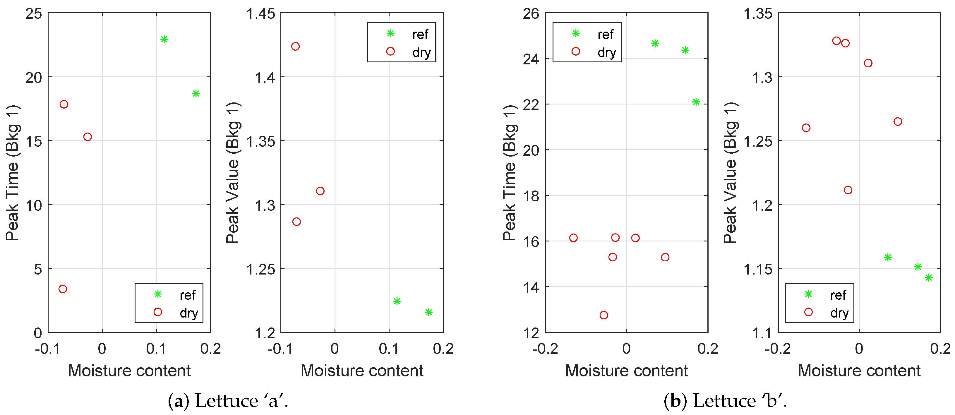
The peak time also decreased for the salt-stressed plants as time passed (Figure 6a, Bkg 1), a result that could be seen as a sign that the plants were becoming increasingly stressed the longer they were watered with salty water. The moisture content in the soil was measured in 14 of the experiments. Figure 7 shows how the peak time and peak value (for the lowest background light) vary with the moisture content. The results show that the measured moisture contents were indeed lower in the dried pots and that the moisture content was positively correlated with the peak time and negatively correlated with the peak value.

In an additional setup, lettuce ‘c’ and lemon balm were evaluated for salt stress. Higher background light levels were included in this setup (85–760 μmol m⁻² s⁻¹). For the two lower light levels (85 and 215 μmol m⁻² s⁻¹), the results were in line with the previous findings. The fluorescence step response can also be used to distinguish between healthy and stressed plants both for lettuce ‘c’ and for lemon balm, with a shorter peak time and higher peak value for stressed plants. The distinction was even more clear for the lemon balm.

In

Table 2. The peak time and peak values (mean values and standard error of the mean, SEM) of responses at the lowest background light level, for healthy and salt-stressed lemon balm and lettuce ‘c’.

		Peak Time		Peak Value
Lettuce ‘c’	Sample size	Mean	SEM	Mean	SEM
Healthy	14	26.31	2.06	1.107	0.007
Salt treated (day 1)	4	17.75	0.48	1.142	0.015
Salt treated (day 2)	4	17.00	0.82	1.215	0.030
Salt treated (day 4)	4	13.50	0.50	1.278	0.017
Lemon balm
Healthy	16	15.69	0.66	1.145	0.015
Salt treated (day 1)	5	5.60	1.47	1.247	0.045
Salt treated (day 3)	5	3.40	0.24	1.270	0.027

, the peak times and peak values for the lowest background light level are summarized. This shows the mean value and the standard deviation of the mean for each group: healthy and salt stressed (for each measurement day). The differences of the mean values were significant (with a confidence of at least 95%), even when comparing the healthy group with only the “least” stressed group, i.e., salt treated (day 1).

For increasing background light levels, there were less but faster dynamics in the fluorescence step responses. As a consequence, the peak value occurred within the first or second sample for all measurements at the two highest background light levels (465 and 760 μmol m⁻² s⁻¹), and for the salt-stressed plants also at the 215 μmol m⁻² s⁻¹ light level. Furthermore, the steady-state level of the fluorescence was not reached within the 4 min that the light was held constant, in contrast to the two lower light levels, where either steady-state was reached or the remaining transients were very small. This also complicates the automation of the data treatment.

To conclude, these experiments shows that it is indeed possible to detect salt and drought stress with proximal measured fluorescence dynamics at the canopy level and that it is preferable to have a background light of 200 μmol m⁻² s⁻¹ or less.

3.2. Pythium Ultimum

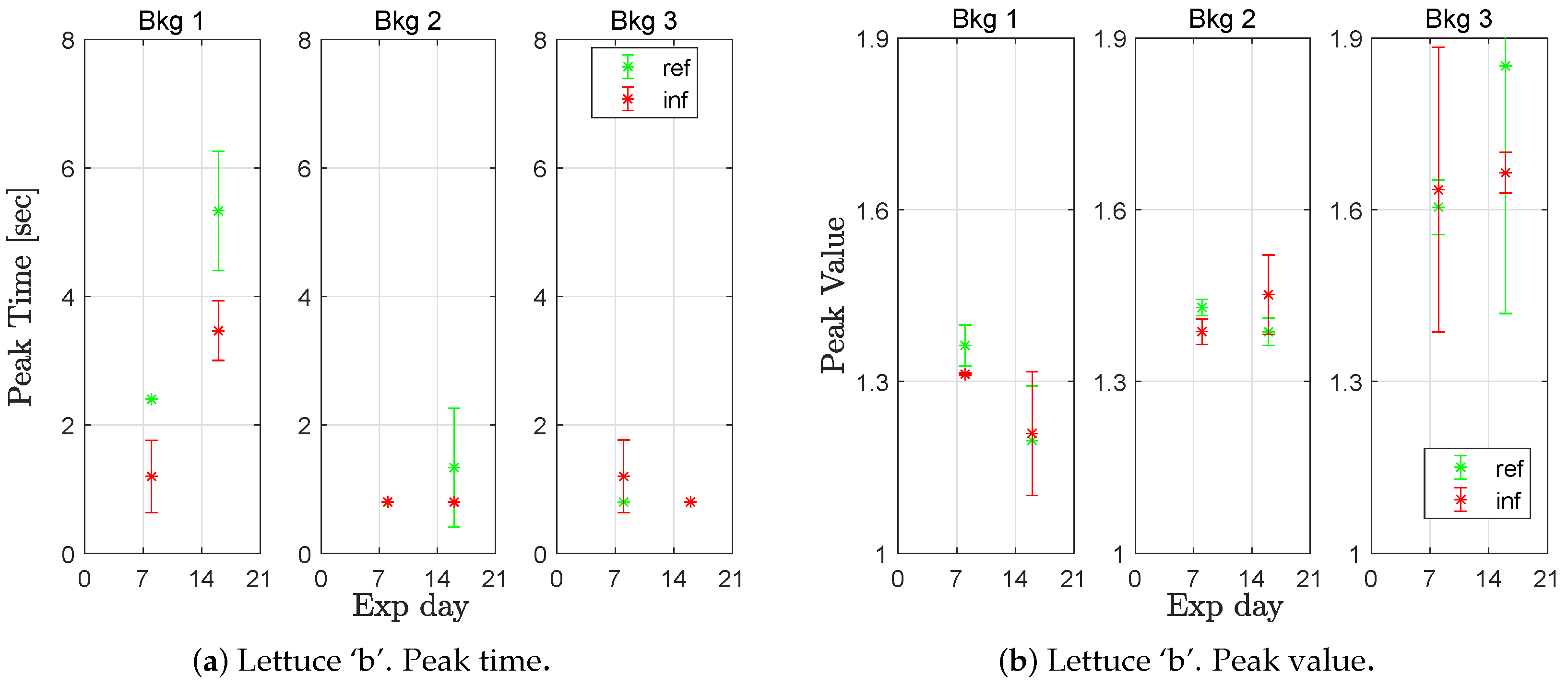
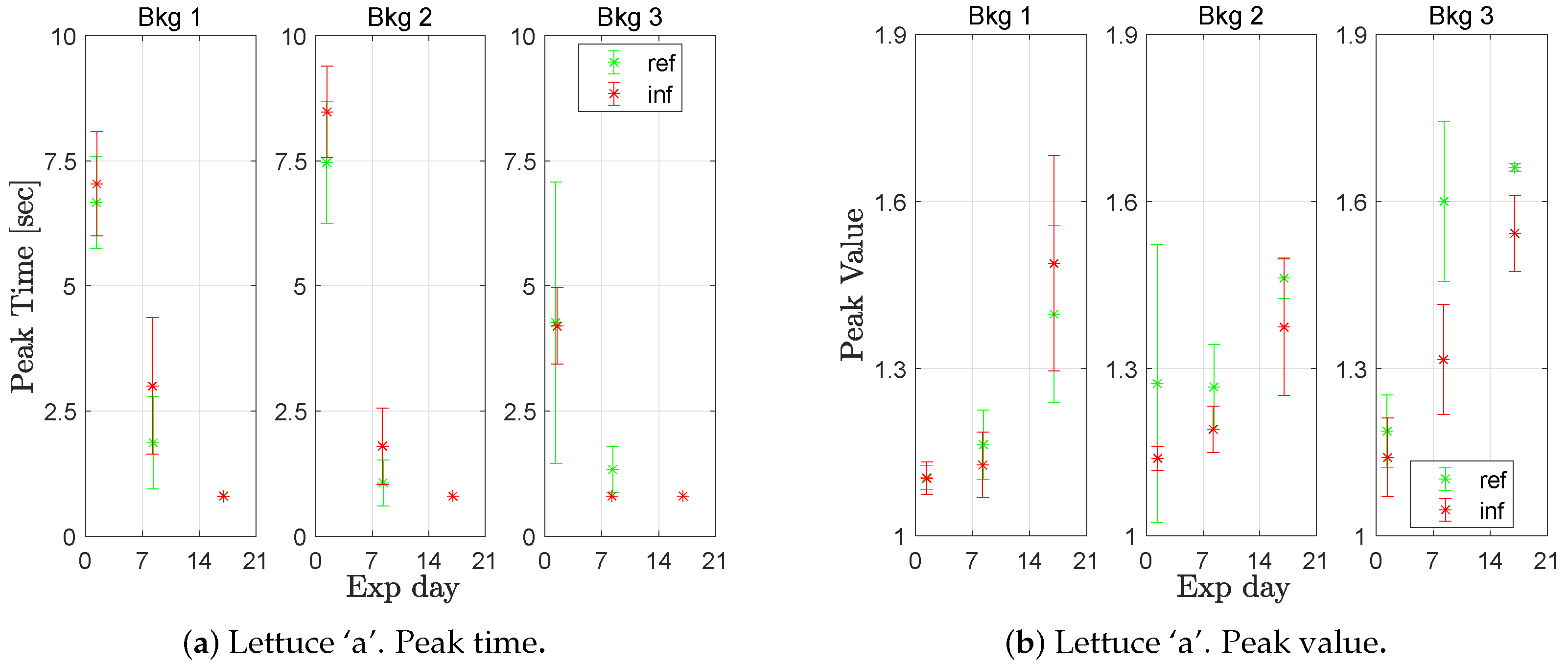
The fluorescence step responses were measured once a week for three weeks, starting the week the pathogens were added (except for lettuce ‘b’, where only measurements from the last two weeks are available). Figure 8 shows the peak time as well as the corresponding peak value of the responses of lettuce ‘b’ for the three different background light intensities.

For each week, the peak time was lower in the infected group compared to the reference group, at the lowest background light level (Bkg 1). The difference was significant at a confidence level of 0.95 for week 3 but not week 2 (but at a confidence level of 0.90, it was). At higher background light, the majority of the registered peak times are at the first sample, making comparisons meaningless. All values are available in Appendix A (

Table A2. Two way ANOVA table, comparing peak times and peak values for healthy (Ref) or Pythium ultimum infected (Inf) lettuce ‘b’. G: Ref week 2 (w 2), H: Inf w 2, I: Ref w 3, and J: Inf w 3.

Comparison		Bkg Light	df	tstat	sd	p	h
Group	Parameter
G and H	peak time	1	2	3.01	0.40	0.095	0
G and H	peak time	2	2	−1.57	0.00	0.256	0
G and H	peak time	3	2	−1.00	0.40	0.421	0
G and H	peak value	1	2	1.98	0.03	0.186	0
G and H	peak value	2	2	2.28	0.02	0.150	0
G and H	peak value	3	2	−1.17	0.18	0.880	0
I and J	peak time	1	4	3.12	0.73	0.036	1
I and J	peak time	2	4	1.00	0.66	0.374	0
I and J	peak time	3	4	0.48	0.00	0.656	0
I and J	peak value	1	4	−1.15	0.10	0.889	0
I and J	peak value	2	4	−1.54	0.05	0.198	0
I and J	peak value	3	4	0.74	0.31	0.498	0

). The peak value, on the other hand, showed no distinction between the healthy and infected groups. Note that the sample size was small (four measures for week 2 and six measures for week 3); therefore, more data is needed to confirm differences with a high level of significance.

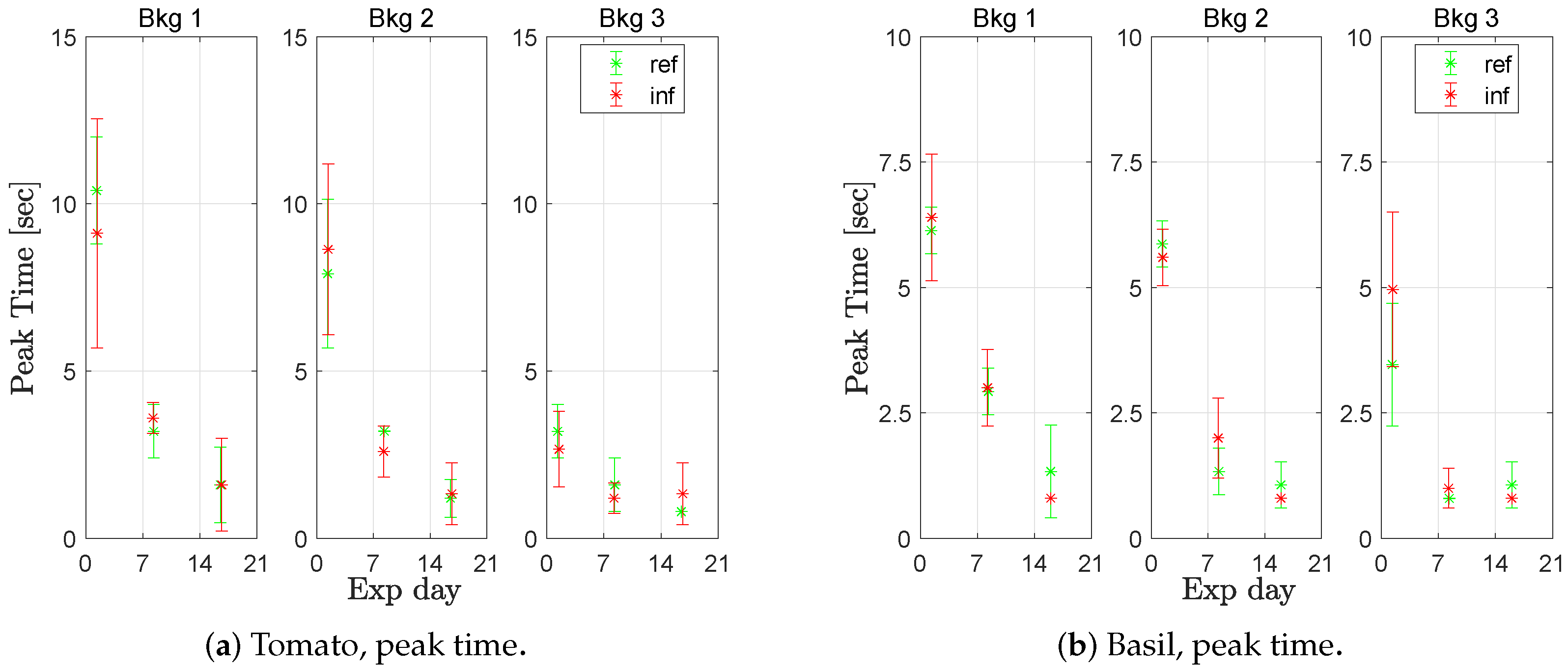
For lettuce ‘a’, basil, and tomato, it was not possible to distinguish between healthy and infected plants when inspecting the fluorescence step responses (Figure 9 and Figure 10). However, the response parameters changed over time such that the peak time decreased and the peak value increased over the three weeks. Comparing the peak times from all measurements week 1 with week 2 or 3, they significantly (at a confidence level of 0.95) different for lettuce ‘a’, basil, and tomato, at all background light levels. The peak values significantly differed when comparing the measurements of week 1 with week 3, for all species and at all background light levels. Data are available in Appendix A (

Table A3. Two way ANOVA table, comparing the peak times and peak values for weeks (w) 1, 2, and 3, for plant in the Pythium ultimum setup. Plants are divided into groups independent of being infected or not. Stress is detected over time, and the authors believe that heat stress is detected. K: tomato, week 1 (w 1), L: tomato, w 2, M: tomato, w 3. N: basil, w 1, O: basil, w 2, P: basil, w 3. Q: lettuce ‘a’, w 1, R: lettuce ‘a’, w 2, and S: lettuce ‘a’, w 3.

Comparison		Bkg Light	df	tstat	sd	p	h
Group	Parameter
K and L	peak time	1	13	5.68	2.10	7.5 $\times {10}^{-5}$	1
K and L	peak time	2	13	6.12	1.74	3.7 $\times {10}^{-5}$	1
K and L	peak time	3	12	3.53	0.81	0.004	1
K and L	peak value	1	13	−1.61	0.10	0.003	1
K and L	peak value	2	13	−1.79	0.10	0.002	1
K and L	peak value	3	12	−1.12	0.23	0.009	1
K and M	peak time	1	11	6.00	2.34	8.9 $\times {10}^{-5}$	1
K and M	peak time	2	11	6.60	1.88	3.9 $\times {10}^{-5}$	1
K and M	peak time	3	10	3.46	0.87	0.006	1
K and M	peak value	1	11	−1.67	0.10	9.7 $\times {10}^{-6}$	1
K and M	peak value	2	11	−1.92	0.11	1.0 $\times {10}^{-4}$	1
K and M	peak value	3	10	−1.89	0.13	6.3 $\times {10}^{-4}$	1
N and O	peak time	1	13	7.68	0.84	3.5 $\times {10}^{-6}$	1
N and O	peak time	2	13	12.47	0.62	1.3 $\times {10}^{-8}$	1
N and O	peak time	3	13	5.86	1.15	5.6 $\times {10}^{-5}$	1
N and O	peak value	1	13	−1.36	0.17	0.724	0
N and O	peak value	2	13	−1.06	0.08	0.009	1
N and O	peak value	3	13	−1.55	0.24	0.146	0
N and P	peak time	1	12	11.14	0.87	1.1 $\times {10}^{-7}$	1
N and P	peak time	2	12	19.83	0.44	1.5 $\times {10}^{-10}$	1
N and P	peak time	3	12	5.36	1.20	1.7 $\times {10}^{-4}$	1
N and P	peak value	1	12	−1.07	0.19	0.306	1
N and P	peak value	2	12	−1.40	0.10	8.7 $\times {10}^{-4}$	1
N and P	peak value	3	12	−1.45	0.22	0.172	1
Q and R	peak time	1	13	7.68	1.10	3.5 $\times {10}^{-6}$	1
Q and R	peak time	2	13	13.69	0.93	4.2 $\times {10}^{-9}$	1
Q and R	peak time	3	12	4.83	1.24	4.1 $\times {10}^{-4}$	1
Q and R	peak value	1	13	−1.72	0.04	0.108	0
Q and R	peak value	2	13	−1.55	0.12	0.590	0
Q and R	peak value	3	12	−1.60	0.13	0.004	1
Q and S	peak time	1	12	15.57	0.73	2.5 $\times {10}^{-9}$	1
Q and S	peak time	2	12	16.31	0.83	1.5 $\times {10}^{-9}$	1
Q and S	peak time	3	11	4.88	1.26	4.9 $\times {10}^{-4}$	1
Q and S	peak value	1	12	−1.77	0.11	8.8 $\times {10}^{-5}$	1
Q and S	peak value	2	12	−1.25	0.13	0.007	1
Q and S	peak value	3	11	−12.55	0.06	7.3 $\times {10}^{-8}$	1

).

At the end of the experiment, the lettuce and basil had passed the appropriate harvest day, and the tomato would have required transplanting for optimal development. The measurements were made in a sunny period when it was warm in the greenhouse. On Day 1, the temperature varied from 19 °C at night up to 28.5 °C at noon. On day 4, the range had increased to 20–31 °C. Unfortunately, further temperature measurements were lost; however, the authors believe the increasing indication of stress (shorter peak time and higher peak value) with time is a heat stress response.

The reference measurements are summarized in

Table 3. Reference measurements in the Pythium ultimum experiment. Mean values with standard deviations within parenthesis of three measurements in each set.

	DW	Pathogen	Maximal Photosynthetic Rate
			Day 11	Day 19
	g	CFU g−1 DW Root	μmolCO2m−2s−1
Tomato
Healthy	10.13 (2.65)		10.9 (1.80)	8.8 (0.65)
Infected	5.94 (5.23)	6.822 (0.009)	9.0 (0.99)	5.4 (3.73)
Basil
Healthy	8.00 (0.31)		14.7 (3.59)	6.6 (0.64)
Infected	7.30 (1.50)	5.599 (0.019)	12.7 (2.69)	8.1 (1.25)
Lettuce ‘a’
Healthy	15.07 (1.31)		8.5 (2.53)
Infected	16.54 (0.96)	6.543 (0.077)	3.6 (2.28)
Lettuce ‘b’
Healthy	8.53 (1.30)
Infected	7.65 (0.72)	7.538 (0.069)

; dry weight (DW; of the leaves, stems, and roots), the amount of pathogen on the roots (per dry weight roots) and the maximal photosynthetic rate. Each set contains three measurements, and the mean values and the standard deviations (according to Equation (2)) are presented in the table.

All plant species (except lettuce ‘a’) had a lower dry weight in the infected group. However, the differences were small and not significant, indicating that the infection did not have a large impact on the photosynthesis of the whole plant. The amount of pathogens on the roots differed significantly between the different plant species. The highest amount was found in lettuce ‘b’, whereas the lowest amount was found in basil.

This is in line with that it was only for lettuce ‘b’ where a statistically significant difference in the peak time was detected between healthy and Pythium infected plants. The maximal photosynthetic rate was measured on basil, tomato, and lettuce ‘a’ on day 11, and again on tomato and basil on day 19.

In line with the expectations that were concluded from the dry weight measurements, the photosynthetic rate measurements only indicated a slightly lower photosynthetic rate for the infected plants (and only in four out of five groups, where a group refers to one species and one measurement day), and the differences were not significant. However, there was a significant decrease in photosynthesis between day 11 and day 19. Hence, the maximal photosynthetic rate appeared to decrease more over time than as a consequence of the Pythium infection in this experiment.

3.3. Powdery Mildew, Podospaera Aphanis

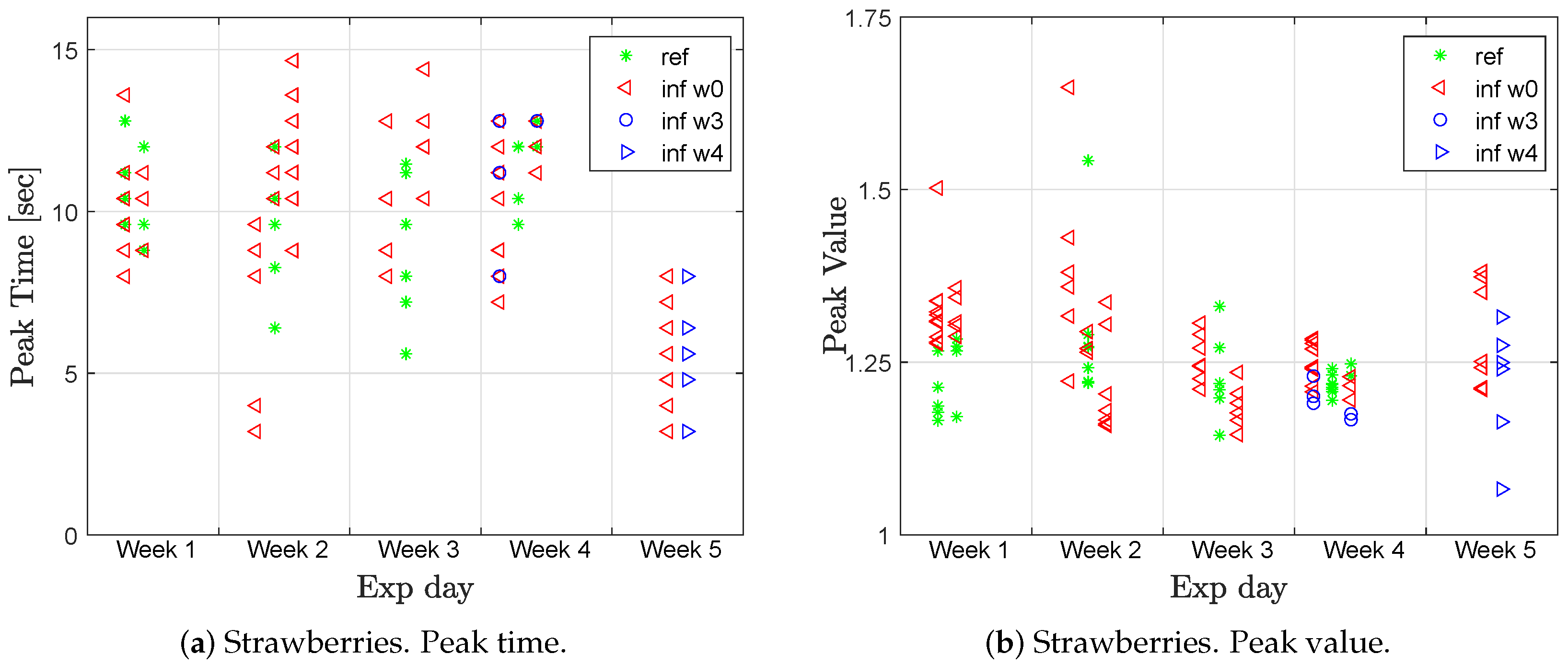
In this setup, over 150 measurements were conducted in order to collect enough data to be used in a supervised machine learning classification algorithm. Unfortunately, the spread of powdery mildew was slower and more uneven than expected, thus, making it difficult to correctly label the data collected in the middle of the experiment.

For the first group of plants that were exposed to the infection—group w0—the infection started four days before the experiment started, i.e., week 0. They were placed in another (slightly warmer) room in the greenhouse, and, when the experiment started, all strawberries were moved to one out of two identical rooms in a closed environment. The intention was to infect more plants over the course of the experiment by moving them into the "infected room" after being subjected to fluorescence step response measurements.

In the same way, group w1 refers to the group that were infected during week 1, after being measured as reference. However, the infection did not evolve as anticipated.

Table 4. Powdery mildew experiment. Numbers of plants that visually showed signs of infection (Inf 1: very light symptoms and Inf 2: slightly more symptoms). The total amount of plants decreases over time as the plants are harvested.

Day	10	15	17	22	30
Group w0
No sign	26	12	6	2	0
Inf 1	3	12	18	14	3
Inf 2	0	2	2	6	13
% infected	10%	54%	77%	91%	100%
Group w1
No sign	18	13	13	11	5
Inf 1	1	3	3	2	1
Inf 2	0	0	0	0	0
% infected	6%	19%	19%	15%	17%

shows the number of plants that visually showed signs of infection during the experiment. Inf 1 corresponds to very light symptoms and Inf 2 to slightly more symptoms (Figure 3). A few plants were harvested every week, hence, there were decreasing total numbers of plants (the harvested leaves were frozen as a backup for possible PCR-measurements to quantify the infection level). As a consequence of the low degree of infection, group w1 was excluded from the presentation of the data.

Figure 11 shows the peak value and peak time for the fluorescence step response after the first excitation at the lowest background light level (110 μmol m⁻² s⁻¹). The results are similar for the second excitation (same background light level). For the third and fourth excitations (both at light level 215 μmol m⁻² s⁻¹) the mean value of the peak time was slightly lower, and the mean value of the peak value was slightly higher.

Four groups are included in the presented figure: the reference group (green stars), infected week 0 (red triangles), and infected weeks 3/4 (blue circles/triangles). Hence, the plants of the blue marks had only been in the infected room for one week and had no visible symptoms, yet, in contrast to group w0 in these weeks, would be expected to behave more similar to the healthy group than the infected group. However, there was no clear distinction between the healthy and infected groups, as shown in Figure 11.

The peak time for most of the measurements were around 10 s, which is relatively high, indicating that the plants appeared to be healthy. The only significant change was in week 5, when the peak time decreased to around 5 s. This could be an indication of higher stress than the previous weeks and this occurred for plants in both groups. Looking at the mean of the peak value, there was only a distinction between the two groups during week 1 and week 5 (

Table 5. Powdery mildew experiment. Peak values at the first background light level, for ref and infected plants at week 1 and week 5.

		Peak Value
Week	Group	Mean	Std	Sem
1	ref	1.223	0.049	0.016
1	inf w0	1.326	0.055	0.014
5	inf w3/4	1.218	0.090	0.037
5	inf w0	1.279	0.076	0.027

). The peak value was then higher for the infected plants.

During week 5, there were visible symptoms of powdery mildew in the infected group (and not in the reference group). Hence, it cannot be excluded that it was the powdery mildew infection that caused the differences in peak values. However, as the differences in peak values between the infected/healthy were not consistent throughout the whole experiment, it is unlikely that the difference in week 1 is due to the infection.

4. Discussion

The aim with this study was to test the hypothesis that it is possible to distinguish between healthy and stressed plants from variations in the dynamic fluorescence response (DFR). The DFR method applied here to detect stress is a modification of the method proposed in Carstensen et al. to analyse the level of light stress [31]. In that work, transfer function responses were fitted to the step responses, and then the transfer functions were analysed in the frequency domain using Bode plots. When applying this to the data presented here, an automated fitting was difficult to achieve, and therefore the time responses were analysed instead—more specifically, the peak time and the normalized peak value.

These two features alone were sufficient to distinguish between healthy and abiotically stressed plants (drought and salt stress investigated), where faster dynamics (shorter peak time) and a higher normalized peak value were found to be indicators of stress. This stress response is also in agreement with the light stress experiments by Carstensen et al. [30,31]. Hence, we concluded that abiotic stress (salt and drought) could be distinguished from healthy plants using DFR.

The experiments with biotic stress unfortunately have certain deficiencies. In particular, this is the case in the set with Pythium ultimum infection; the sample size is small, a few reference measurements are lacking, and the plants were grown in a warm greenhouse, which likely led to heat stress. Generally, no significant difference could be detected between healthy and Pythium infected plants, with the applied DFR-method. Hence, we could not confirm the hypothesis for this stressor. It was only for lettuce ‘b’ that the mean value of the peak time varied as a function of plant status; however, due to the small sample size, it is difficult to confirm differences with a high level of significance.

However, the measurements of pathogens on the roots showed that these were the plants with the highest occurrence of pathogens. Therefore, and due to the nature of the infection, i.e., a root infection that is difficult to visually detect, we suggest more research to determine if there is a critical level of infection required, in order for the method to work for detection of Pythium infection. Furthermore, in a stress detection setting where several step responses are measured (for example, several step responses every night), it is easier to detect differences compared to only singular measurements as was done in this study.

The plants in the Pythium setup were grown in a warm greenhouse, and we detected a significantly higher stress the third week compared to the first week, for all species included. It was likely heat stress that was detected, even though it cannot be excluded that it could be something else, such as malnutrition. Unfortunately, there is no data to either confirm or reject this. It was warm in the greenhouse during the Pythium experiments: day one had a 28.5/19 °C day/night temperature, and day four was 31/20 °C. Unfortunately, subsequent temperature data was lost; however, the outdoor weather continued to be warm and sunny, and this was the case also in the greenhouse.

The measurements of the maximal photosynthetic rate (data for five out of eight plant species and days were available), indicated a slight decrease as a consequence of Pythium infection in most of the measurements; however, the decrease was larger when comparing measurements from day 19 and with the ones from day 11 (Table 3). The fact that the photosynthetic apparatus was only slightly affected by the infection but more affected over time can (at least partly) explain the fact that the proposed fluorescence detection method captured a difference over time (increased heat stress) but could not distinguish between healthy and infected samples.

For powdery mildew on strawberries, a pilot study with heavily infected plants indicated that the peak time and the peak value could be used to separate healthy and infected plants. However, in the main experiment, the plants were never infected to the same degree, and it was also not possible to distinguish between the two groups, except from the peak value measurements during week 1 and week 5 (Table 5). Potentially, this was due to the infection in week 5; however, as the difference was not detected throughout the whole experiment, there is likely another explanation for the difference in week 1.

To start the infection, group w0 had to be moved to another room in the greenhouse (to ensure no infection of the reference group), in which the temperature was about 5 °C higher. This was done four days prior to the start of the experiment when all plants were moved to the controlled, indoor environment. The difference in the fluorescence step response in the two groups during week 1 may, therefore, be because they reacted differently to the movement from the greenhouse to the indoor environment, either due to the powdery mildew or due to the different temperatures that they were exposed to in the greenhouse.

The method proposed here only measures the mean value of the fluorescence response over the entire canopy (two plants for the powdery mildew setup). Consequently, to be detected, a considerable part of the canopy must be affected. This is beyond the limit of acceptance for a detection method for powdery mildew. As this infection starts with a local infection, it would likely be more efficient to use a sensor with higher spatial resolution, e.g., a fluorescence camera. Possibly one could then detect specific areas of the plant that have a deviating step response signatures due to the infection.

The intention of using a machine learning algorithm to extract the most important features for classification of healthy/infected strawberry plants was unfortunately not possible. The infection did not spread at the rate that we expected, which led to uncertain annotation of the plants. However, it may still work to use the dynamic fluorescence response to generate input features to a classification algorithm. In such an algorithm, additional features can be added to increase the performance and to solve the problem of finding a general threshold value of, for example, the peak time or peak value, to classify plants as healthy or not. Candidate features to investigate could be the ambient conditions (temperature, humidity, etc.), plant status (age, development state, species, etc.), or other features from the fluorescence dynamics.

In the presented method, we measured the transient behaviour of chlorophyll fluorescence. However, this is slightly different from standard methods, in the sense that we did not include dark adaption. A dark-adapted leaf that is illuminated with continuous (or modulated) excitation shows a characteristic change in chlorophyll a fluorescence intensity over time [36]. This is called the fluorescence transient, or the Kautsky effect, named after Hans Kautsky, who first reported this phenomenon in 1931 [37].

The fast part of this transient occurs within the first second of illumination and is called the OJIP transient curve; the fluorescence level at origin (O), followed by two intermediates (I, J) and finally the peak (P). The following, slower dynamics, SMT (semi-steady state, maximum, and terminal steady-state), occurs on the time scale of minutes [38].

Due to the current sample rate we used, normally 0.8 s, we could not capture the behaviour of the fast transient (OJIP). Instead, the peak that we follow is likely something that is similar to the second maximum, M. A previous study on bean leaves [39] reported that the time of the M-peak decreased for an increased heat stress on the leaves. This is clearly in line with our results, in that a short peak time indicated plant stress.

Another finding from the conducted experiments, was that the distinction between healthy and stressed plants was easier to detect at low background light intensities. The higher the background light level, the faster the dynamics in the fluorescence step response for all plants, no matter the stress status, thus, making it difficult to distinguish between them, at least with the current sampling rate. This can be seen in Figure 6, Figure 8, Figure 9, and Figure 10, comparing the peak time at the first background light level with the latter ones.

Previous research on dark adapted pea leaves, showed that the shape of the fluorescence transient curve was very different depending on the excitation light level [40]. The excitation light from a LED with peak wavelength at 650 nm, at approximately 30, 300, and 3000 μmol m⁻² s⁻¹ were investigated. For the highest light, the slope from P to T was smooth, whereas, in the case of the lowest light, the semi-steady state S and second maximum M were pronounced. In our setup, we did not elaborate on the excitation light (it was always within 30–70 μmol m⁻² s⁻¹); however, in addition to the excitation light, we also had different background light levels.

Our finding—that the dynamics became faster at higher background light levels—might actually be the transition from a fluorescence curve where the M-peak is pronounced (low light) to the case where there is a smooth decrease from the P-peak to the terminal steady state, T. Hence, at the higher background light, there was no “M-peak” to detect and, instead, the maximal value occurred in the “P-peak”, which is within our first measured sample.

5. Conclusions

A method for plant stress detection is presented where the measurements can be done on-line, remotely on the canopy level, and the plants neither need to be dark adapted nor exposed to saturating light. Furthermore, the equipment can be relatively simple. For this research, a spectrometer was used; however, a simpler, cheaper type of photodiode with a bandpass optical filter could be applicable, and, in such a case, could be distributed over a large greenhouse. Furthermore, ordinary (controllable) LED growth lights, already in place in many advanced greenhouses, were used to supply the (relatively weak) blue light used to excite a fluorescence response.

The results from this research show that the abiotic stress from drought and salt (and probably heat), can efficiently be detected by the suggested method. The examined biotic stress from powdery mildew Podosphaera aphanis (on strawberries) and the root infection Pythium ultimum (on two types of lettuce, basil, and tomato) could not be significantly distinguished from healthy plants.

However, the results indicate that, for a severe infection, the stress appeared to be detectable. For the root infection case, the disease is difficult to detect visually, and hence this is an interesting option. More experiments are then needed to determine if there is a critical level of infection for detection and, then, to decide whether it is an acceptable limitation or not.

Powdery mildew, on the other hand, does not affect the whole plant at the start—instead, it spreads point-wise. Due to that nature, it will likely be more efficient to have a sensor with higher spatial resolution as it is desired to detect the mildew already at a stage when it is only visible on very small spots on single leaves.

References

1. Shamshiri, R.R.; Kalantari, F.; Ting, K.C.; Thorp, K.R.; Hameed, I.A.; Weltzien, C.; Ahmad, D.; Shad, Z.M. Advances in greenhouse automation and controlled environment agriculture: A transition to plant factories and urban agriculture. Int. J. Agric. Biol. Eng. 2018, 11, 1–22. [Google Scholar] [CrossRef]
2. Sankaran, S.; Mishra, A.; Ehsani, R.; Davis, C. A review of advanced techniques for detecting plant diseases. Comput. Electron. Agric. 2010, 72, 1–13. [Google Scholar] [CrossRef]
3. Simko, I.; Hayes, R.J.; Furbank, R.T. Non-destructive phenotyping of lettuce plants in early stages of development with optical sensors. Front. Plant Sci. 2019, 7, 1985. [Google Scholar] [CrossRef] [PubMed] [Green Version]
4. Galieni, A.; D’Ascenzo, N.; Stagnari, F.; Pagnani, G.; Xie, Q.; Pisante, M. Past and Future of Plant Stress Detection: An Overview From Remote Sensing to Positron Emission Tomography. Front. Plant Sci. 2021, 11, 1975. [Google Scholar] [CrossRef] [PubMed]
5. Porcar-Castell, A.; Tyystjarvi, E.; Atherton, J.; van der Tol, C.; Flexas, J.; Pfundel, E.E.; Moreno, J.; Frankenberg, C.; Berry, J.A. Linking chlorophyll a fluorescence to photosynthesis for remote sensing applications: Mechanisms and challenges. J. Exp. Bot. 2014, 65, 4065–4095. [Google Scholar] [CrossRef]
6. Murchie, E.H.; Lawson, T. Chlorophyll fluorescence analysis: A guide to good practice and understanding some new applications. J. Exp. Bot. 2013, 64, 3983–3998. [Google Scholar] [CrossRef] [PubMed] [Green Version]
7. Schreiber, U. Pulse-Amplitude-Modulation (PAM) Fluorometry and Saturation Pulse Method: An Overview. In Chlorophyll a Fluorescence: A Signature of Photosynthesis; Papageorgiou, G.C., Ed.; Springer: Dordrecht, The Netherlands, 2004; pp. 279–319. [Google Scholar] [CrossRef]
8. Meroni, M.; Rossini, M.; Guanter, L.; Alonso, L.; Rascher, U.; Colombo, R.; Moreno, J. Remote sensing of solar-induced chlorophyll fluorescence: Review of methods and applications. Remote Sens. Environ. 2009, 113, 2037–2051. [Google Scholar] [CrossRef]
9. Aasen, H.; Van Wittenberghe, S.; Sabater Medina, N.; Damm, A.; Goulas, Y.; Wieneke, S.; Hueni, A.; Malenovský, Z.; Alonso, L.; Pacheco-Labrador, J.; et al. Sun-Induced Chlorophyll Fluorescence II: Review of Passive Measurement Setups, Protocols, and Their Application at the Leaf to Canopy Level. Remote Sens. 2019, 11, 927. [Google Scholar] [CrossRef] [Green Version]
10. Oerke, E.C.; Mahlein, A.K.; Steiner, U. Proximal Sensing of Plant Diseases. In Detection and Diagnostics of Plant Pathogens; Gullino, M.L., Bonants, P.J.M., Eds.; Springer: Dordrecht, The Netherlands, 2014; pp. 55–68. [Google Scholar] [CrossRef]
11. Kolber, Z.; Klimov, D.; Ananyev, G.; Rascher, U.; Berry, J.; Osmond, B. Measuring photosynthetic parameters at a distance: Laser induced fluorescence transient (LIFT) method for remote measurements of photosynthesis in terrestrial vegetation. Photosynth. Res. 2005, 84, 121–129. [Google Scholar] [CrossRef]
12. Keller, B.; Vass, I.; Matsubara, S.; Paul, K.; Jedmowski, C.; Pieruschka, R.; Nedbal, L.; Rascher, U.; Muller, O. Maximum fluorescence and electron transport kinetics determined by light-induced fluorescence transients (LIFT) for photosynthesis phenotyping. Photosynth. Res. 2019, 140, 221–233. [Google Scholar] [CrossRef] [Green Version]
13. Raesch, A.R.; Muller, O.; Pieruschka, R.; Rascher, U. Field Observations with Laser-Induced Fluorescence Transient (LIFT) Method in Barley and Sugar Beet. Agriculture 2014, 4, 159–169. [Google Scholar] [CrossRef] [Green Version]
14. Urschel, M.R.; Pocock, T. Remote Detection of Growth Dynamics in Red Lettuce Using a Novel Chlorophyll a Fluorometer. Agronomy 2018, 8, 227. [Google Scholar] [CrossRef] [Green Version]
15. Zhang, J.; Huang, Y.; Pu, R.; Gonzalez-Moreno, P.; Yuan, L.; Wu, K.; Huang, W. Monitoring plant diseases and pests through remote sensing technology: A review. Comput. Electron. Agric. 2019, 165, 104943. [Google Scholar] [CrossRef]
16. Polonio, l.; Pineda, M.; Bautista, R.; Martínez-Cruz, J.; Pérez-Bueno, M.L.; Barón, M.; Pérez-García, A. Rna-seq Analysis and Fluorescence Imaging of Melon Powdery Mildew Disease Reveal an Orchestrated Reprogramming of Host Physiology. Sci. Rep. 2019, 9, 7978. [Google Scholar] [CrossRef] [PubMed] [Green Version]
17. Römer, C.; Bürling, K.; Hunsche, M.; Rumpf, T.; Noga, G.; Plümer, L. Robust fitting of fluorescence spectra for pre-symptomatic wheat leaf rust detection with Support Vector Machines. Comput. Electron. Agric. 2011, 79, 180–188. [Google Scholar] [CrossRef]
18. Pineda, M.; Pérez-Bueno, M.L.; Paredes, V.; Barón, M. Use of multicolour fluorescence imaging for diagnosis of bacterial and fungal infection on zucchini by implementing machine learning. Funct. Plant Biol. 2017, 44, 563–572. [Google Scholar] [CrossRef] [PubMed] [Green Version]
19. Kuska, M.T.; Mahlein, A.K. Aiming at decision making in plant disease protection and phenotyping by the use of optical sensors. Eur. J. Plant Pathol. 2018, 152, 987–992. [Google Scholar] [CrossRef]
20. Mohd Asaari, M.S.; Mishra, P.; Mertens, S.; Dhondt, S.; Inzé, D.; Wuyts, N.; Scheunders, P. Close-range hyperspectral image analysis for the early detection of stress responses in individual plants in a high-throughput phenotyping platform. Isprs J. Photogramm. Remote Sens. 2018, 138, 121–138. [Google Scholar] [CrossRef]
21. Moghimi, A.; Yang, C.; Marchetto, P.M. Ensemble Feature Selection for Plant Phenotyping: A Journey From Hyperspectral to Multispectral Imaging. IEEE Access 2018, 6, 56870–56884. [Google Scholar] [CrossRef]
22. Behmann, J.; Bohnenkamp, D.; Paulus, S.; Mahlein, A.K. Spatial Referencing of Hyperspectral Images for Tracing of Plant Disease Symptoms. J. Imaging 2018, 4, 143. [Google Scholar] [CrossRef] [Green Version]
23. Behmann, J.; Mahlein, A.K.; Rumpf, T.; Roemer, C.; Pluemer, L. A review of advanced machine learning methods for the detection of biotic stress in precision crop protection. Precis. Agric. 2015, 16, 239–260. [Google Scholar] [CrossRef]
24. Sun, D.; Zhu, Y.; Xu, H.; He, Y.; Cen, H. Time-Series Chlorophyll Fluorescence Imaging Reveals Dynamic Photosynthetic Fingerprints of sos Mutants to Drought Stress. Sensors 2019, 19, 2649. [Google Scholar] [CrossRef] [PubMed] [Green Version]
25. Blumenthal, J.; Megherbi, D.B.; Lussier, R. Unsupervised machine learning via Hidden Markov Models for accurate clustering of plant stress levels based on imaged chlorophyll fluorescence profiles & their rate of change in time. Comput. Electron. Agric. 2020, 174, 105064. [Google Scholar] [CrossRef]
26. Ahlman, L.; Bånkestad, D.; Wik, T. LED spectrum optimisation using steady-state fluorescence gains. Acta Hortic. 2016, 1134, 367–374. [Google Scholar] [CrossRef]
27. Ahlman, L.; Bånkestad, D.; Wik, T. Using chlorophyll a fluorescence gains to optimize LED light spectrum for short term photosynthesis. Comput. Electron. Agric. 2017, 142, 224–234. [Google Scholar] [CrossRef]
28. Ahlman, L.; Bånkestad, D.; Wik, T. Relation between Changes in Photosynthetic Rate and Changes in Canopy Level Chlorophyll Fluorescence Generated by Light Excitation of Different Led Colours in Various Background Light. Remote Sens. 2019, 11, 434. [Google Scholar] [CrossRef] [Green Version]
29. Bånkestad, D.; Wik, T. Growth tracking of basil by proximal remote sensing of chlorophyll fluorescence in growth chamber and greenhouse environments. Comput. Electron. Agric. 2016, 128, 77–86. [Google Scholar] [CrossRef]
30. Carstensen, A.M.; Pocock, T.; Bånkestad, D.; Wik, T. Remote detection of light tolerance in Basil through frequency and transient analysis of light induced fluorescence. Comput. Electron. Agric. 2016, 127, 289–301. [Google Scholar] [CrossRef]
31. Carstensen, A.M.; Wik, T.; Bånkestad, D.; Pocock, T. Exploring the dynamics of remotely detected fluorescence transients from basil as a potential feedback for lighting control in greenhouses. Acta Hortic. 2016, 1134, 375–384. [Google Scholar] [CrossRef]
32. Lindqvist, J.; Bånkestad, D.; Carstensen, A.M.; Lundin, B.; Wik, T. Complexity of Chlorophyll Fluorescence Dynamic Response as an Indicator of Excessive Light Intensity. IFAC-PapersOnLine 2016, 49, 392–397. [Google Scholar] [CrossRef]
33. Hultberg, M.; Alsanius, B.; Sundin, P. In Vivo and in Vitro Interactions between Pseudomonas fluorescens and Pythium ultimum in the Suppression of Damping-off in Tomato Seedlings. Biol. Control. 2000, 19, 1–8. [Google Scholar] [CrossRef]
34. Montgomery, D. Design and Analysis of Experiments, 7th ed.; Student Solutions Manual; John Wiley & Sons: Hoboken, NJ, USA, 2009. [Google Scholar]
35. Khalil, S.; Beatrix, W.A. Effect of growing medium water content on the biological control of root pathogens in a closed soilless system. J. Hortic. Sci. Biotechnol. 2011, 86, 298–304. [Google Scholar] [CrossRef]
36. Papageorgiou, G.C. (Ed.) Chlorophyll a Fluorescence A Signature of Photosynthesis; Springer: Dordrecht, The Netherlands, 2004; Volume 19. [Google Scholar]
37. Kautsky, H.; Hirsch, A. Neue Versuche zur Kohlensäureassimilation. Naturwissenschaften 1931, 19, 964. [Google Scholar] [CrossRef]
38. Stirbet, A.; Govindjee. On the relation between the Kautsky effect (chlorophyll a fluorescence induction) and Photosystem II: Basics and applications of the OJIP fluorescence transient. J. Photochem. Photobiol. Biol. 2011, 104, 236–257. [Google Scholar] [CrossRef] [PubMed]
39. Levykina, I.P.; Karavaev, V.A. Fluorescence induction changes in bean leaves after heat treatment. Biophys. Med. Phys. 2016, 71, 128–134. [Google Scholar] [CrossRef]
40. Strasser, R.J.; Srivastava, A.; Govindjee. Polyphasic chlorophyll a fluorescent transient in plants and cyanobacteria. Photochem. Photobiol. 1995, 61, 32–42. [Google Scholar] [CrossRef]
Figure 1. (a) Incident light (background and excitation) within PAR, repeated for four different background light levels. (b) Fluorescence signal (integrated over wavelengths 720–760 nm).
Agriengineering 03 00042 g001
Figure 2. Arrows showing the peak time and the peak value. The peak value is the maximal value of the normalized fluorescence. The peak time is the time evolved from the time the excitation light is added until the peak value is reached.
Agriengineering 03 00042 g002
Figure 3. Powdery mildew infected plants; left—reference plant without visual symptom, middle—infected level 1, and right—infected level 2.
Agriengineering 03 00042 g003
Figure 4. The fluorescence response of the first excitation for all biotic stress experiments on lettuce ‘a’. Green dotted lines: healthy reference plants. Orange solid lines: salt-stressed plants. Red dashed lines: drought-stressed plants.
Agriengineering 03 00042 g004
Figure 5. Peak time (a) and peak value (b) of the responses at all four background light levels for healthy (ref) as well as the salt- and drought-stressed lettuce ‘a’.
Agriengineering 03 00042 g005
Figure 6. Peak time (a) and peak value (b) of the fluorescence step response for measurements on lettuce ‘b’; healthy (green star), as well as salt (red triangle) and dry (red circle) stressed. The first subplot (on a and b) corresponds to the lowest background light level (Bkg 1).
Agriengineering 03 00042 g006
Figure 7. Peak time and peak value at the lowest background light level vs. the relative moisture content (higher value more irrigated) for (a) lettuce ‘a’ and (b) lettuce ‘b’.
Agriengineering 03 00042 g007
Figure 8. The fluorescence step response peak time (a) and peak value (b) for lettuce ‘b’ at three different background light levels. The mean value and std for two to five measurements each week and for each group (reference and infected with Pythium ultimum).
Agriengineering 03 00042 g008
Figure 9. The fluorescence step response peak time (a) and peak value (b) for lettuce ‘a’ at three different background light levels. The mean value and std for two to five measurements each week and for each group (reference and infected with Pythium ultimum).
Agriengineering 03 00042 g009
Figure 10. The fluorescence step response peak time for tomato (a) and basil (b) at three different background light levels. The mean value and std for two to five measurements each week and for each group (reference and infected with Pythium ultimum).
Agriengineering 03 00042 g010
Figure 11. Fluorescence step response (a) peak time and (b) peak value for powdery mildew infected strawberries at the lowest background light level. ref: healthy plants, inf w0: infected week 0, i.e., 4 days prior to first measurement, inf w3/4: measured as reference weeks 3/4, after being placed in the infected unit but with no visual symptoms.
Agriengineering 03 00042 g011