Article

Spatial Prediction of Agrochemical Properties on the Scale of a Single Field Using Machine Learning Methods Based on Remote Sensing Data †

Institute of Environmental Sciences, Kazan Federal University, Kremlevskaya Str. 18, 420008 Kazan, Russia
*
Author to whom correspondence should be addressed.
Presented at the 1st International Electronic Conference on Agronomy, 3–17 May 2021; Available online: https://sciforum.net/conference/IECAG2021; accessed on 7 November 2021.
Submission received: 29 September 2021 / Revised: 31 October 2021 / Accepted: 4 November 2021 / Published: 9 November 2021

Abstract

:
Creating accurate digital maps of the agrochemical properties of soils on a field scale with a limited data set is a problem that slows down the introduction of precision farming. The use of machine learning methods based on the use of direct and indirect predictors of spatial changes in the agrochemical properties of soils is promising. Spectral indicators of open soil based on remote sensing data, as well as soil properties, were used to create digital maps of available forms of nitrogen, phosphorus, and potassium. It was shown that machine learning methods based on support vectors (SVMr) and random forest (RF) using spectral reflectance data are similarly accurate at spatial prediction. An acceptable prediction was obtained for available nitrogen and available potassium; the variability of available phosphorus was modeled less accurately. The coefficient of determination (R2) of the best model for nitrogen is R2SVMr = 0.90 (Landsat 8 OLI) and R2SVMr = 0.79 (Sentinel 2), for potassium—R2SVMr = 0.82 (Landsat 8 OLI) and R2SVMr = 0.77 (Sentinel 2), for phosphorus—R2SVMr = 0.68 (Landsat 8 OLI), R2SVMr = 0.64 (Sentinel 2). The models based on remote sensing data were refined when soil organic matter (SOC) and fractions of texture (Silt, Clay) were included as predictors. The SVMr models were the most accurate. For Landsat 8 OLI, the SVMr model has a R2 value: nitrogen—R2 = 0.95, potassium—R2 = 0.89 and phosphorus—R2 = 0.65. Based on Sentinel 2, nitrogen—R2 = 0.92, potassium—R2 = 0.88, phosphorus—R2 = 0.72. The spatial prediction of nitrogen content is influenced by SOC, potassium—by SOC and texture, phosphorus—by texture. The validation of the final models was carried out on an independent sample on soils from a chernozem zone. For nitrogen based on Landsat 8 OLI R2 = 0.88, for potassium R2 = 0.65, and for phosphorus R2 = 0.31. Based on Sentinel 2, for nitrogen R2 = 0.85, for potassium R2 = 0.62, and for phosphorus R2 = 0.71. The inclusion of SOC and texture in remote sensing-based machine learning models makes it possible to improve the spatial prediction of nitrogen, phosphorus and potassium availability of soils in chernozem zones and can potentially be widely used to create digital agrochemical maps on the scale of a single field.

1. Introduction

The widespread introduction into agricultural practice of the digital technologies of variable-rate fertilizers is currently one of the conditions for gross crop production with a minimal negative impact on the environment [1]. Furthermore, the technology of variable rate fertilization helps to increase the ability of the soil to store carbon [2].
Precision farming technologies are focused on the optimal satisfaction of the nutrient needs of cultivated plants, taking into account the spatial heterogeneity of arable land in terms of agrochemical indicators. At the same time, the need for precision farming technologies requires the development of new approaches to the description of the spatial heterogeneity of soil cover.
When conducting research related to soil degradation and pollution, modeling of the spatial heterogeneity of soil cover by various parameters is often carried out on a national and regional scale [3,4,5,6,7,8,9]. However, the practice of soil cover mapping for the implementation of precision farming systems usually requires a description of the soil heterogeneity of arable land on the scale of one definite field, often using a limited set of point data [10,11]. The transfer of models of spatial heterogeneity of soils to different-scale objects is a very difficult and as yet unresolved task [12]. Therefore, the formation of approaches to the creation of maps of the heterogeneity of arable land for precision farming should be considered as an independent problem requiring a separate solution.
Ordinary kriging has traditionally been used in interpolated agrochemical maps for precision farming [1], which can offer certain disadvantages if the dataset is limited. Webster and Oliver [13] believe that when using kriging, at least 100 data are required for successful variogram calculations. Kerry et al. [14] admitted that, using special variogram modeling methods, it is possible to limit the processing of 50 spatially localized data. At the same time, Saito and Goovaerts [15] note that when using fewer than 50 (or even 100 observations), the kriging method may not offer any obvious advantages over other interpolators. It is also necessary to take into account the fact that an increase in the number of points due to a decrease in the area of soil sampling sites to create more reliable maps of spatial variability presents difficulties associated with the significant increase in the costs of sampling in the field and conducting the analyses [16].
It is natural that when developing methodological support for precision agriculture, emphasis is placed on approaches to creating maps of spatial heterogeneity of arable land soils based on the use of predictors that allow the minimization of the number of soil samples and at the same time provide denser coverage of the entire field. In this respect, Goovaerts et al. [17] considered the possibility of using cokriging and regression kriging for precision farming. Regression kriging is one of the most popular, practical, and reliable methods of hybrid spatial interpolation, which makes it possible to model the distribution of soil properties across space and time [18,19,20]. For example, Lin et al. [21] showed that the use of logistic regression and regression kriging provides a more reliable assessment of the risk of soil contamination with heavy metals for monitoring information support than spatial probabilistic models. Despite all its advantages, the productive use of regression kriging for solving precision farming problems may also present limitations, which are primarily related to the compilation of a set of spatially localized data and the indirect predictors used. Hengl et al. [19] recommend using regression kriging only for data sets with more than 50 observations and at least 10 observations for each predictor of multiple regression, which prevents over-fitting of the model. On the chernozem soils of Tatarstan (Russia), we have previously shown that the use of regression models based on kriging to create large-scale maps of soil properties offers advantages over ordinary kriging only if a sufficiently large number of predictors (at least more than 10) is used for modeling [22]. As a limitation of the regression kriging method, it can also be noted that when describing the deterministic part of the variability of the target variable, it is not always possible to take into account the nonlinear nature of the effect of predictors. The limitations and advantages of this method are discussed in detail in the review by Keskin and Grunwald [20].
Recently, there has been an increasing interest in soil science in machine learning and deep learning methods, as well as data mining methods, which can significantly improve the accuracy of spatial predictions [23]. For example, an improvement in the accuracy of spatial prediction using machine learning methods was obtained when mapping soil pollution with various pollutants [9,24,25,26], the content and organic matter stocks [3,4,11,27,28], and physicochemical and agrochemical soil properties [29,30]. In general, various machine learning algorithms offer similar indicators of spatial prediction [7,27], but a reasonable choice of algorithm for modeling a specific soil property with a certain set of predictors still allows us to improve the final result [7].
The advantages of using machine learning, deep learning, and data mining methods in comparison with traditional methods of spatial analysis are often manifested on the global [29], national [6], and regional scaling levels [31,32,33,34]. On the scale of individual fields, which is necessary for the application of variable-rate fertilizer, machine learning methods are used less often. [12,35]. Recently, Matinfar et al. [11] obtained acceptable accuracy from their spatial prediction of SOC on the scale of a separate field by using machine learning methods in combination with covariates of remote sensing. Many studies are related to the analysis of soil properties and vegetation conditions at different scales, in which satellite data are successfully used [10,36,37,38,39,40]. Nevertheless, digital mapping of the heterogeneity of the soil properties of arable land, based on the use of remote sensing data, is largely determined by their availability [17]. Currently, the widely used Landsat 8 OLI and Sentinel 2 satellites, which are publicly available, offer different, but acceptable, resolutions and feature a wide range of reflectance bands in various spectrum ranges. Thus, this work is aimed at assessing the possibility of using remote sensing data obtained from the Landsat 8 OLI and Sentinel 2 satellites as predictors of the spatial prediction of the agrochemical properties of the soil on the field scale when using machine learning methods.

2. Materials and Methods

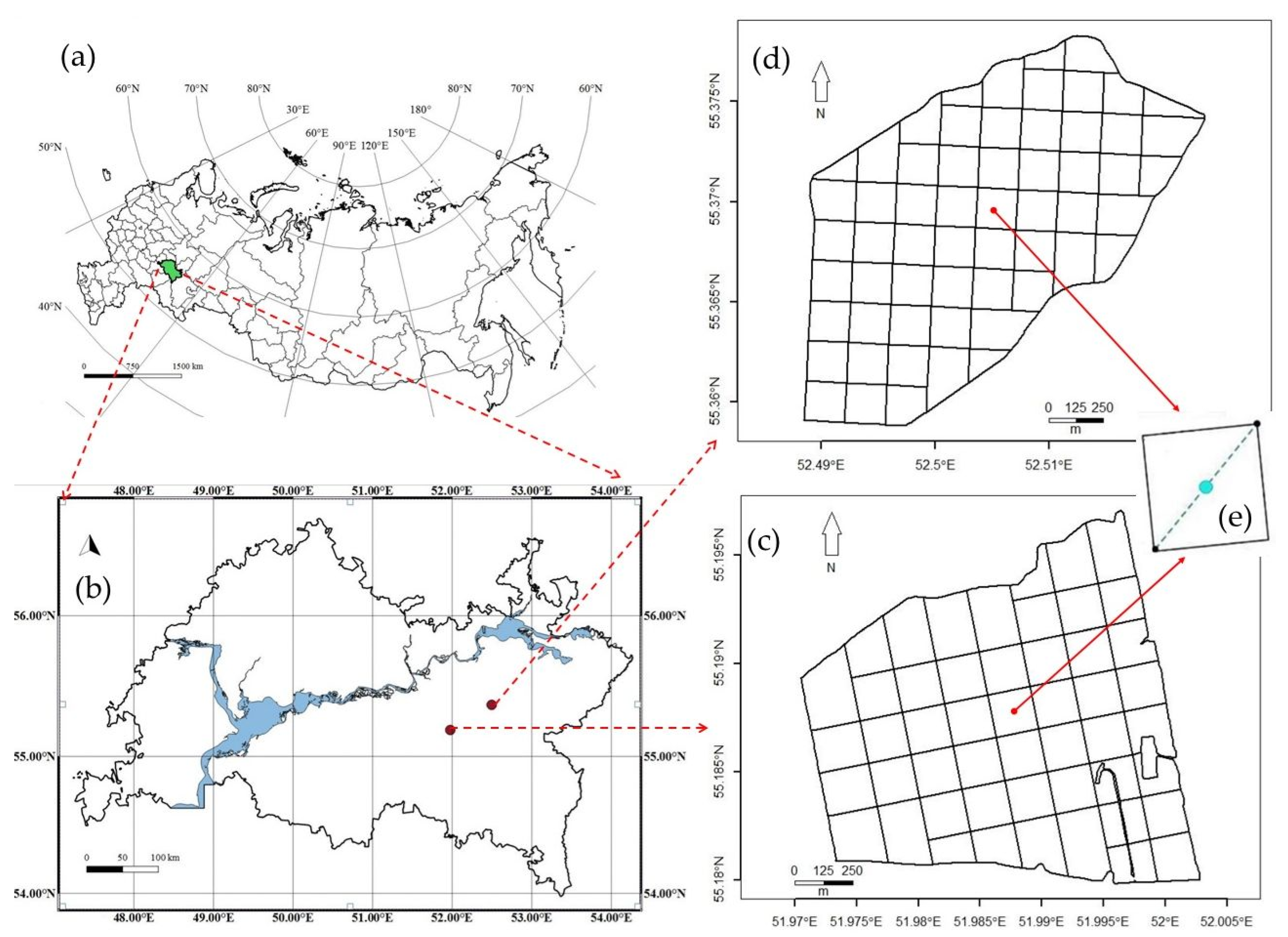
2.1. Study Area and Sampling Design

Two fields located on the territory of the Republic of Tatarstan (Russia) in the zone of chernozem soils were used as the object (Figure 1). Tatarstan is located in the eastern part of the East European Plain, within forest and forest-steppe natural zones. Umbric Albeluvisols, Albic Luvisols, and Chernozems are widespread in these zones.
The need to model the agrochemical properties of chernozem soils is primarily due to the fact that the introduction of advanced technologies in agriculture offers great benefits when applied to more fertile soils. Precision farming technologies are no exception and their introduction into practice in Russia occurs mainly in the zone of distribution of chernozem soils. The first field (55.182893° N, 51.999358° E) with an area of 254 hectares is characterized by a height difference of up to 60 m, with steep slopes and high soil heterogeneity and fertility. The second field (52.49621° N, 55.35032° E), with an area of 287 hectares, is characterized by a smaller dissection of the relief (a height difference of 30 m) and a more homogeneous soil cover. The first field was used to train the model, while the second field was used to test the final models.
The fields were divided into elementary square plots with a size of about 5 hectares, from which point samples (20–40 pieces each) were taken in 2019 to compile mixed samples. In total, 50 mixed samples were compiled for the first field, and 59 for the second field. The content of available forms of nitrogen for plants according to Cornfield (N), phosphorus (P2O5), and potassium (K2O), according to the Chirikov method, were determined in the samples. The Cornfield method is based on long-term alkaline (1 mol L−1 NaOH) hydrolysis of the soil at optimal temperature and humidity, followed by the determination of the released NH3. The determination of phosphorus and potassium by the Chirikov method is a standard method for assessing the content of available forms in noncarbonate chernozem soils. The method is based on soil treatment with 1 mol L−1 acetic acid. The organic carbon content in the samples was determined by dry combustion on an organic elemental analyzer Vario Max Cube (Elementar, Langenselbold, Germany). The fractions of silt and clay were determined by laser diffraction on a BLUEWAVE particle size analyzer (Microtrac, York, PA, USA) after soil treatment with sodium pyrophosphate and dispersion of suspensions by ultrasound. All reagents were purchased from Ecopharm, Kazan, Russia.

2.2. Remote Sensing Data and Spectral Indices

The sources of the remotely sensed datasets were from the Landsat 8 OLI and Sentinel 2 satellites, which were obtained from the websites of the US Geological Survey and the European Space Agency. Images with open soil, i.e., with minimal influence of vegetation, were used for the work. For Landsat 8 OLI, the images used were from 31 May 2019. For the Sentinel 2 satellite, the images were from 12 May 2019. During the selection of the satellite images, the minimal influence of atmospheric disturbances was taken into account; however, all the images were subjected to atmospheric correction using the DOS 1 method (dark object subtraction). The DOS 1 method assumes that there are areas within the satellite image where the reflection coefficient is almost zero (water, dense forest, shadow). The signal from these areas is the result of atmospheric scattering, which must be removed. The difference between this value and the actual value of the digital numbers of images (DN) can be attributed to the additive haze effect [41].
Based on the satellite data, spectral indices were calculated that characterize open soil and may reflect the redistribution of soil material, and may also correlate with such fundamental soil properties as SOC and texture. In chernozem soils, these are the main properties of soils that determine the availability of nitrogen, phosphorus, and potassium. Table 1 shows a list of the indices used and their calculation formulas, which were adapted for the Landsat 8 OLI and Sentinel 2 satellites. Individual satellite bands (Landsat 8 OLI: Bands 2–7, Sentinel 2: Bands 1–8, 11 and 12) and bands ratios were also used for the spatial prediction of agrochemical properties. The data of each satellite were used separately from each other.
Texture can be characterized by Cli and GSI indices and MID-Infrared index (MID-IR). Open soil can be characterized by both low NDVI values and bare soil indices (BSI 1, BSI 2) and indices that determine the color indicators of soils (RI, BI, SI, CI). SOC may have a relationship with the panchromatic index and the indices of bare soil. Agricultural cultivation of soil cover and non-photosynthetic vegetation, which are determined by the indices NDI 1, NDI 2, can also affect the color characteristics of soils.
The values of the spectral data were extracted from the polygons of the elementary sampling sites and averaged. The average remote sensing data and laboratory data were linked to the coordinates of the centroids of the sampling polygons.

2.3. Spatial Prediction Methods

For the spatial prediction, regression models based on Support Vectors (SVMr) and Random Forest (RF) were used. Regression based on support vectors is a controlled nonparametric machine learning method. The method is based on the use of the nonlinear transformation technique to map the original input space into a new hyperspace [52]. In the transformed hyperspace, complex and nonlinear relations between covariates and the output variable can be modeled using a linear function [53]. The SVMr model defines a decision boundary, which restricts points that are close to the hyperplane. The support vectors are involved in finding the closest match between the data points and the actual function that they represent. Due to its ability to process nonlinear relations and efficiency in generalization, SVMr has shown itself to be a promising method in various soil studies [30,54,55].
An RF is a tree-like machine learning algorithm that, using the results of several decision trees, can significantly reduce the risk of overfitting. The algorithm is based on the construction of decision trees, which are then combined according to certain criteria to create random forests. RF can be generated from hundreds (or even thousands) of decision trees. The predictions in RF are generated as the average of predictions of an ensemble of decision trees. The decision tree constructed each time may differ due to randomness; this uniqueness is used as an advantage to model multiple nonlinear relationships [56,57]. Random selection and averaging procedures make RF models stable algorithms with a high predictive ability [58]. RF is mainly used for classification tasks; several comparative studies have proven that this is one of the best and currently available machine learning methods [57].
The correlations of the remote sensing data with the target soil’s properties were investigated using the Spearman correlation. Since the set of potential predictors was large, a subsample of data was created using the Recursive Feature Elimination (RFE) procedure to obtain the most important predictors for each response variable. For each model, the importance estimates of the predictors were iteratively determined, and were then ranked according to the degree of importance for the response variable. At each stage of the search, the least important predictors were iteratively removed before the next stage in the creation of the model. The corresponding estimation functions were used for the models. The size of the subsample corresponding to the best value of the objective function was used as the final model [59].
The RF and SVMr models were subjected to a tuning procedure. For the RF models, the optimal values of the number of variables at each moment of tree separation (“mtry”) were estimated. Accordingly, a random search for the values was performed within the range of the predictors using 10-fold cross-validation and estimation by the corresponding performance indicator [60]. A total of 1000 trees were selected as the “ntree” parameter.
For the SVMr models, the ε-insensitive error function “epsilon”, and the penalty parameter “cost”, which regulates the excess of this error, were tuned. The radial basis function was used as the core function. The model was tuned using a 10-fold cross-validation with an assessment based on the performance indicator.
The models were tested using the bootstrap procedure with replacement and taking into account the optimism which characterizes the overfitting of the model [60]. The approach consists of the following steps:
  • Fitting the model to the original data and evaluating the performance indicator.
  • Getting a bootstrap sample with replacement from the original data.
  • Fitting the model to the bootstrap dataset and evaluating the performance indicator.
  • Fitting the model from the bootstrap dataset to the original dataset and evaluating the performance indicator.
  • Evaluation of optimism by the average value of the difference in the performance indicator of the model from point 3 and the model from point 4.
  • Evaluation of the performance indicator adjusted for optimism by subtracting the value of the optimism from the performance indicator of the model from point 1.
The model evaluation measures were the RMSE, MAE, and R2 criteria.
Mean absolute error:
MAE = 1 n i   = 1 n | ( p i o i ) |
Root-mean-square error:
RMSE = [ 1 n i   = 1 n ( p i o i ) 2 ] 1 / 2
Coefficient of determination:
R 2 = 1 i   = 1 n ( o i p i ) 2 i   = 1 n ( o i   o ¯ ) 2
where pi is the predicted value and oi is the observed value.
The best models were recognized as models with a minimum value of RMSE and MAE and a maximum value of R2.

2.4. Software

Atmospheric correction of remote sensing data was carried in the Semi-Automatic classification plugin in QGIS [61]. Statistical analysis, correlation analysis, modeling, and working with rasters were carried out using the object-oriented language R [62]. The correlation matrix was plotted using the “corrplot” package. Work with raster images was carried out in the “raster” package. The RF models were built using the “randomForest” package and the SVMr models were built using the “kernlab” and “e1071” packages. The models were tuned using the “caret” package.

3. Results and Discussion

3.1. Descriptive Statistics

Table 2 shows the statistical data of the soil properties. The variation of available nitrogen on the training field is characterized as average with a range of variation of 91.8 mg kg−1. The variability of the available phosphorus content was very high; the range of variation was 206.7 mg kg−1. The variation in the available potassium was average, with a range of variation of 192.9 mg kg−1.
The variability of available nitrogen in the test field was average, with an average value of 140.0 mg kg−1. The available potassium demonstrated a strong variability, with an average value of 163.3 mg kg−1, and the available phosphorus was characterized by very high variability and an average value of 131.3 mg kg−1. According to the agrochemical indicators, both fields were similar. Differences were observed in silt and clay. The variability of the silt content on the training field was low, with a range of variation of 47.8%. In terms of clay content, the field was heterogeneous, with very high variability; the range of variation was 18.5%. On the test field, the coefficient of variation showed very weak variability for silt (4%), and weak variability for clay (10%). The SOC content on the training field was characterized by the average spatial variation (range of variation 2.9%). The SOC content on the test field was 1.5 times higher than on the training field.

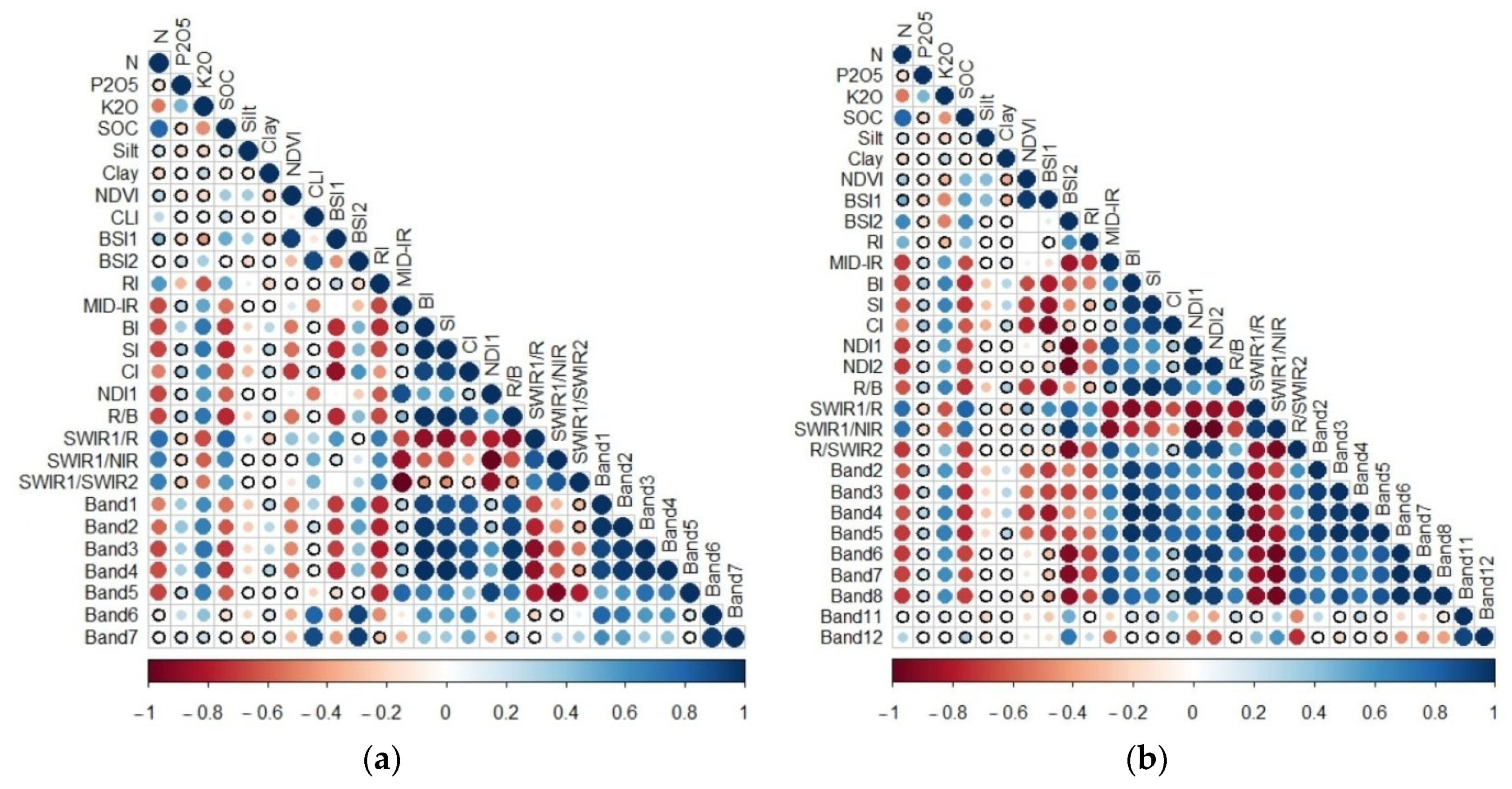
3.2. Correlation Relations

Figure 2 shows the correlation matrices of the relationships between the soil properties and the remote sensing data. Nitrogen had the strongest relationship with SOC (r = 0.80), and low correlation with clay r = −0.21 and silt—r = 0.20. The correlation of nitrogen with SOC was statistically significant (p < 0.05), whereas with texture it was not significant.
Furthermore, the available phosphorus and potassium demonstrated a low correlation with texture. Silt demonstrated a correlation with phosphorus r = −0.19 and with potassium—r = 0.22. Clay correlated with potassium r = 0.25; the correlation of available phosphorus with clay was very low. The correlation of texture with phosphorus and potassium was not significant at 5% significance level.
Of the agrochemical properties, the available nitrogen and available potassium correlated the strongest with the remote sensing data. The available nitrogen displayed mostly negative correlations with the remote sensing data. The significant values (p < 0.05) of the correlation coefficient for nitrogen in the case of Landsat 8 OLI ranged from r = −0.51 to r = −0.68, and in the case of Sentinel 2 from r = −0.50 to r = −0.72. A significant (p < 0.05) positive correlation of nitrogen with the remote sensing data was also present and varied in a range from r = 0.28 to r = 0.75 for Landsat 8 OLI and from r = 0.47 to r = 0.75 for Sentinel 2. The available potassium displayed the most significant (p < 0.05) positive correlation with individual bands: from r = 0.51 to r = 0.74 for Landsat 8 OLI and from r = 0.56 to r = 0.69 for Sentinel 2. The correlation of the available phosphorus with the remote sensing data was mostly positive, but low. For Landsat 8 OLI, the significant correlation (p < 0.05) of phosphorus varied from r = 0.24 to r = 0.4. In the case of Sentinel 2, the correlation of phosphorus with the remote sensing data was not significant at 5% significance level.

3.3. Accuracy of Remote Sensing-Based Models

Table 3 shows an estimate of the accuracy of models of spatial variability of the content of the available forms of nitrogen, phosphorus, and potassium. When using RF and SVMr models, based on Sentinel 2 data, the content of available nitrogen and available potassium were predicted more accurately. For the available nitrogen, the SVMr model (Sentinel 2) demonstrated the value R2 = 0.79 and the RF model—R2 = 0.77; the determination coefficient of the SVMr model for the available potassium R2 = 0.77, and the RF model—R2 = 0.62. When using the Landsat 8 OLI satellite data for the available nitrogen, the SVMr model displayed the value R2 = 0.90 and the RF model—R2 = 0.74. For the available potassium, the value of the determination coefficient of the SVMr model (Landsat 8 OLI) corresponded to R2 = 0.82 and the RF model—R2 = 0.66. The models of the spatial variability of the available phosphorus were less effective. In the case of the Landsat 8 OLI satellite data, for the available phosphorus when using the SVMr model, the value R2 = 0.68 and the RF model—R2 = 0.49, whereas, when using the Sentinel 2 data for the SVMr model, R2 = 0.64, and for the RF model—R2 = 0.45.
In general, after a comprehensive assessment of all the modeling accuracy indicators (RMSE, MAE and R2), the results of the spatial modeling using SVMr and RF algorithms based on the satellite data were satisfactory. At the same time, it is necessary to recognize that the accuracy of some modeling results should be improved, especially the supply of soils with available forms of phosphorus.
When attempting to improve spatial prediction, many studies consider the use of different types of predictors (indicators of soil properties, vegetation state, morphometry) for evaluating the target variable [5,11,37]. A significant improvement in spatial prediction when using machine learning methods can be achieved by using individual soil indicators as predictors of spatial data, along with remote sensing materials. For example, Kumar et al. (2011) used interpolated maps of soil properties (clay, total nitrogen, pH, etc.) for a spatial assessment of the SOC stock [63]. To create predictive maps of the SOC content using machine learning and data mining, Were et al. [16] used interpolated maps of the texture, Ca, Mg, P, K, total nitrogen, and pH. It is clear that among soil properties, the change in the content of available forms of nutrients is primarily influenced by the content of SOC and the texture.

3.4. Accuracy of Models Based on Remote Sensing and Soil Properties

Using the existing analytical data, maps of changes in the SOC content, silt fraction, and clay fraction were compiled using SVMr and RF machine learning algorithms based on the remote sensing data. In the case of the Sentinel 2 data, the best prediction was obtained using the RF model (R2 = 0.84), while for the content of silt and clay fractions, the SVMr model was the most effective at prediction (R2 = 0.62 and R2 = 0.76, respectively). In the case of the Landsat 8 OLI data, the RF model was found to be the best for the content of SOC (R2 = 0.83) and clay (R2 = 0.61), and the SVMr model was found to be the most effective for the content of silt (R2 = 0.87). The final maps were used as additional predictors together with the remote sensing data when modeling the variability of the content of the available forms of nitrogen, phosphorus, and potassium.
The inclusion of soil properties in the remote sensing model made it possible to improve the accuracy of the prediction of the nutrients. The exceptions were the variants of the models of the available phosphorus (RF (Sentinel 2), SVMr (Landsat 8 OLI), RF(Landsat 8 OLI)), and available potassium (RF (Sentinel 2), RF (Landsat 8 OLI)). For the remaining variants, there was a noticeable improvement in the accuracy of the prediction when using a combination of remote sensing with soil properties. For example, for Sentinel 2, in the case of available nitrogen, the value of R2 in the RF model increased from 0.77 to 0.83, and in the SVMr model, from 0.79 to 0.92. In the case of potassium, the SVMr showed an improvement in R2 from 0.77 to 0.88, whereas in the case of phosphorus, the R2 of the SVMr model increased from 0.64 to 0.72. For Landsat 8 OLI, a similar situation was also observed for available nitrogen, the R2 of the SVMr model changed from 0.90 to 0.95, and the R2 of the RF model from 0.74 to 0.82. There was also an improvement in the SVMr (Landsat 8 OLI) model for the available potassium; R2 increased from 0.82 to 0.89. For all the variants (from both Landsat 8 OLI and Sentinel 2), the SVMr model offered better predictions compared to the RF models. The SVMr models offered better predictions of the available nitrogen and potassium content than of available phosphorus. The prediction accuracy for phosphorus content in soils when using remote sensing data is low. For example, in a study by Hengl et al. [64] showed of 15 indicators of soils in sub-Saharan Africa, significant models for most target nutrients displayed a value of R2 from 40% to 85% (including total nitrogen and extracted potassium), except phosphorus, sulfur, and boron.
The degree of influence of remote sensing predictors and soil properties on the available forms of nitrogen, phosphorus and potassium, expressed as a weighting factor of each predictor in the SVMr models, is shown in Figure 3. For the available nitrogen, there was a significant influence of SOC, since there were often strong correlations between SOC and N. Of the soil properties, only the content of the silt and clay fractions influenced the available phosphorus, and the combined effect of silt, clay, and SOC influenced the available potassium. The latter was most likely because the availability of potassium is significantly influenced by the content of its exchange forms in the soil, which is largely determined by the cation exchange capacity (CEC) of the soil, and the availability of phosphorus is influenced by the lithology of soil material.

3.5. Validation of the Models Based on an Independent Data Sample

When assessing the reliability of predictive models at describing the spatial heterogeneity of soils on the scale of one field, along with assessing their accuracy, it is necessary to assess the reliability of other, similar objects. Since the transferability of the initial models is largely determined by the regional peculiarities of the formation of the heterogeneity of the soil cover, a field also located in the zone of distribution of chernozems was selected for testing. The final models with the highest R2 values were subjected to the validation procedure. The validation data are presented in Table 4.
In general, the models showed an expected decrease in the accuracy of the spatial prediction. For the nitrogen based on Landsat 8 OLI, the test models demonstrated values of R2 = 0.88 (R2 of the original model = 0.95), for potassium R2 = 0.65 (R2 of the original model = 0.89), and for phosphorus R2 = 0.31 (R2 of the original model = 0.65). Based on Sentinel 2, the test model for nitrogen demonstrated R2 = 0.85 (R2 of the original model = 0.92), for potassium R2 = 0.62 (R2 of the original model = 0.88), and for phosphorus R2 = 0.71 (R2 of the original model = 0.72). It can be assumed that the decrease in the accuracy of the prediction in the test field was associated with a lower degree of terrain indentation and a smaller manifestation of intra-field transfer of soil material compared to the first field used to train the final models. It can also be assumed that to ensure the universality of the resulting models, it is necessary to expand the set of predictors (for example, to include morphometric attributes of the relief). For example, Mponela et al. (2020) showed that phosphorus content has a closer relationship with the attributes of the digital relief model SRTM than with remote sensing; the relationship of relief indicators with potassium content is weaker [65]. At the same time, it should be taken into account that poor prediction can be caused mainly by small sample sizes and high variability of auxiliary predictors [10]. Thus, the choice of a reasonable relationship between these parameters can also produce greater reliability in models.

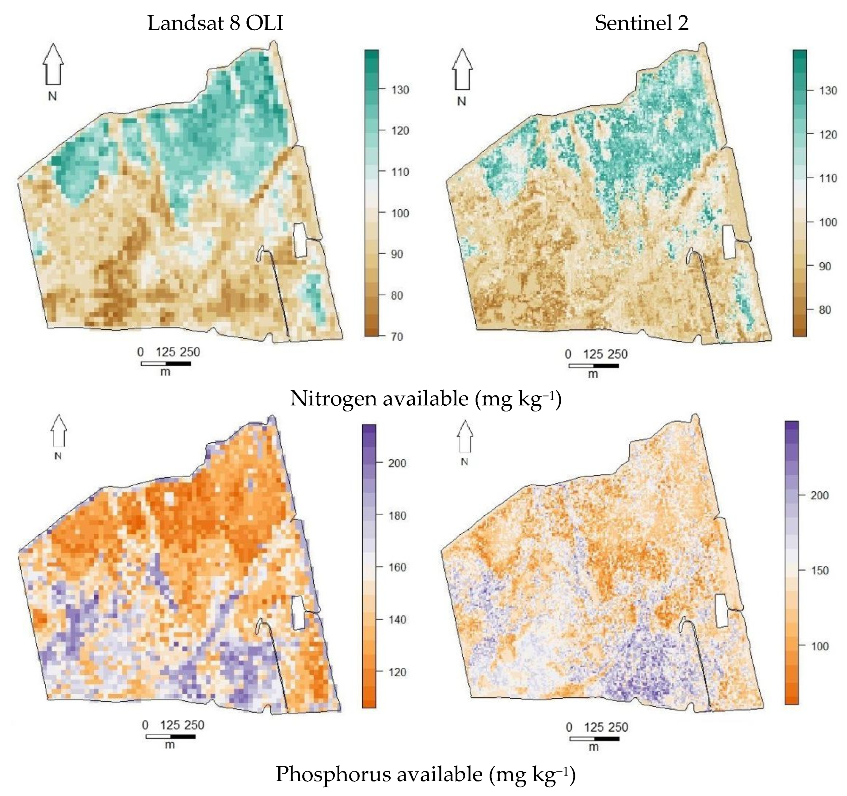
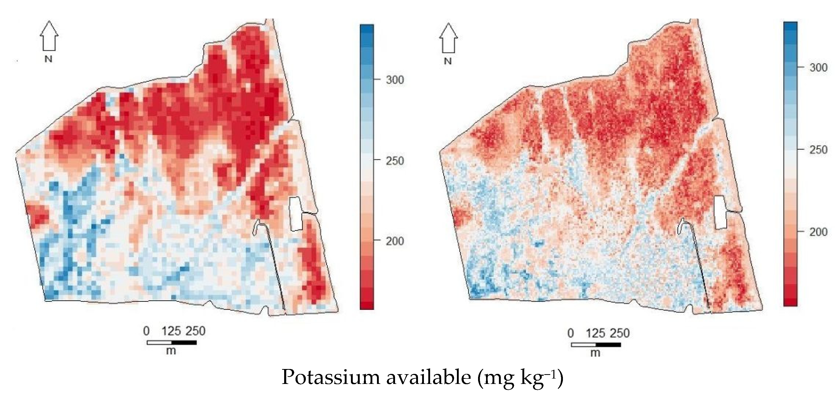
3.6. Final Spatial Prediction Maps

The final maps of the spatial prediction of the available forms of nitrogen, phosphorus, and potassium obtained from the Landsat 8 OLI and Sentinel 2 satellite data, as well as the soil properties using the SVMr models, are shown in Figure 4.
The maps based on Sentinel 2 are characterized by a greater degree of detail on the spatial variability of the soil properties. It is known that Sentinel 2 data are more sensitive to local changes in soil parameters, in contrast to Landsat 8 OLI data, which feature a coarser resolution. Similar conclusions were made in other works, for example, in the study of saline soils in China [66]. At the same time, the accuracy of the prediction according to Landsat 8 OLI data approximately corresponded to the accuracy of the prediction based on Sentinel 2 data, especially when using additional predictors of the soil properties. The similarity of the accuracy of the spatial prediction when mapping changes with the content of SOC using different space sensors (Sentinel 2, Landsat 8, and PlanetScope) was also noted by Žížala, et al. [39]. Thus, when choosing a remote sensing source, it is necessary to take into account the planned accuracy of dosing mineral fertilizers with the technical resources used. Currently, when creating maps for variable-rate fertilization, the planning of application cells with a size of 18 m × 18 m, which is less than the resolution of the Landsat-8 satellite, is considered standard. In such cases, the use of more detailed agrochemical maps created based on the Sentinel 2 satellite data may be considered preferable. For example, a prediction with a resolution of at least 10 m can be useful for the application of precision farming technologies in irrigated agriculture and irrigated vegetable growing.

4. Conclusions

The use of RF and SVMr algorithms based on Landsat 8 OLI and Sentinel 2 data on open chernozem soil for the spatial prediction of available forms of nitrogen, phosphorus, and potassium shows similar performance values. The phosphorus content was predicted to be worse than the nitrogen and potassium content, which were more closely related to the remote sensing data. The available nitrogen displayed mostly negative correlations with the remote sensing data: from r = −0.51 to r = −0.68 (Landsat 8 OLI), from r = −0.50 to r = −0.72 (Sentinel 2). The available potassium demonstrated the most significant positive correlation with the individual bands: from r = 0.51 to r = 0.74 for Landsat 8 OLI and from r = 0.56 to r = 0.69 for Sentinel 2. The correlation of the available phosphorus with the remote sensing data was low.
The inclusion of soil indicators (SOS, silt, clay) in the remote sensing model makes it possible to improve the spatial prediction of nutrients. When modeling remote sensing in combination with soil indicators, the SVMr algorithm produced the best results. The test of the best final models on an independent sample (chernozem) revealed a decrease in the accuracy of R2 compared to the original models. For the nitrogen based on the Landsat 8 OLI, the test models demonstrated values of R2 = 0.88 (R2 of the original model = 0.95), for potassium R2 = 0.65 (R2 of the original model = 0.89), and for phosphorus R2 = 0.31 (R2 of the original model = 0.65). Based on Sentinel 2, the test model for nitrogen demonstrated s R2 = 0.85 (R2 of the original model = 0.92), for potassium R2 = 0.62 (R2 of the original model = 0.88), and for phosphorus R2 = 0.71 (R2 of the original model = 0.72).
To improve the reliability of the model, it is necessary to use additional predictors (for example, morphometric relief attributes), and it is also necessary to take into account the limitation of the model to the zone of applicability. Future research should aim at determining the boundaries of the range of applicability of models. However, models based on one or more fields can be used to survey the entire territory without the additional cost of agrochemical analysis for precision farming purposes.
The need to model the agrochemical properties of chernozem soils is primarily due to the fact that the introduction of advanced technologies in agriculture offers great benefits in more fertile soils. Precision farming technologies are no exception and their introduction into practice in Russia occurs mainly in the zone of distribution of chernozem soils.

Author Contributions

I.S.: formal analysis, visualization, writing—original draft preparation. E.S.: project administration, writing—review and editing. K.G.: investigation, visualization, writing—original draft preparation. All authors have read and agreed to the published version of the manuscript.

Funding

This research was funded by the Russian Foundation for Basic Research, research project № 19-29-05061-mk.

Data Availability Statement

Not applicable.

Conflicts of Interest

The authors declare no conflict of interest. The funders had no role in the design of the study; in the collection, analyses, or interpretation of data; in the writing of the manuscript, or in the decision to publish the results.

References

  1. Oliver, M.A. An Overview of Geostatistics and Precision Agriculture. In Geostatistical Applications for Precision Agriculture; Oliver, M.A., Ed.; Springer: Dordrecht, The Netherlands, 2010; pp. 1–34. [Google Scholar] [CrossRef]
  2. Sozzi, M.; Bernardi, E.; Kayad, A.; Marinello, F.; Boscaro, D.; Cogato, A.; Gasparini, F.; Tomasi, D. On-the-Go Variable Rate Fertilizer Application on Vineyard Using a Proximal Spectral Sensor. In Proceedings of the 2020 IEEE International Workshop on Metrology for Agriculture and Forestry (MetroAgriFor), Trento, Italy, 4–6 November 2020; pp. 343–347. [Google Scholar]
  3. Wiesmeier, M.; Barthold, F.; Blank, B.; Kögel-Knabner, I. Digital Mapping of Soil Organic Matter Stocks Using Random Forest Modeling in a Semi-Arid Steppe Ecosystem. Plant Soil 2011, 340, 7–24. [Google Scholar] [CrossRef]
  4. Kerry, R.; Goovaerts, P.; Rawlins, B.G.; Marchant, B.P. Disaggregation of Legacy Soil Data Using Area to Point Kriging for Mapping Soil Organic Carbon at the Regional Scale. Geoderma 2012, 170, 347–358. [Google Scholar] [CrossRef] [PubMed] [Green Version]
  5. Dai, F.; Zhou, Q.; Lv, Z.; Wang, X.; Liu, G. Spatial Prediction of Soil Organic Matter Content Integrating Artificial Neural Network and Ordinary Kriging in Tibetan Plateau. Ecol. Indic. 2014, 45, 184–194. [Google Scholar] [CrossRef]
  6. Martin, M.P.; Orton, T.G.; Lacarce, E.; Meersmans, J.; Saby, N.P.A.; Paroissien, J.B.; Jolivet, C.; Boulonne, L.; Arrouays, D. Evaluation of Modelling Approaches for Predicting the Spatial Distribution of Soil Organic Carbon Stocks at the National Scale. Geoderma 2014, 223–225, 97–107. [Google Scholar] [CrossRef] [Green Version]
  7. Mahmoudzadeh, H.; Matinfar, H.R.; Taghizadeh-Mehrjardi, R.; Kerry, R. Spatial Prediction of Soil Organic Carbon Using Machine Learning Techniques in Western Iran. Geoderma Reg. 2020, 21, e00260. [Google Scholar] [CrossRef]
  8. Ward, K.J.; Chabrillat, S.; Brell, M.; Castaldi, F.; Spengler, D.; Foerster, S. Mapping Soil Organic Carbon for Airborne and Simulated EnMAP Imagery Using the LUCAS Soil Database and a Local PLSR. Remote Sens. 2020, 12, 3451. [Google Scholar] [CrossRef]
  9. Sakizadeh, M.; Rodríguez Martín, J.A. Spatial Methods to Analyze the Relationship between Spanish Soil Properties and Cadmium Content. Chemosphere 2021, 268, 129347. [Google Scholar] [CrossRef]
  10. Jafari, A.; Khademi, H.; Finke, P.A.; Van de Wauw, J.; Ayoubi, S. Spatial Prediction of Soil Great Groups by Boosted Regression Trees Using a Limited Point Dataset in an Arid Region, Southeastern Iran. Geoderma 2014, 232–234, 148–163. [Google Scholar] [CrossRef]
  11. Matinfar, H.R.; Maghsodi, Z.; Mousavi, S.R.; Rahmani, A. Evaluation and Prediction of Topsoil Organic Carbon Using Machine Learning and Hybrid Models at a Field-Scale. CATENA 2021, 202, 105258. [Google Scholar] [CrossRef]
  12. Grunwald, S.; Yu, C.; Xiong, X. Transferability and Scalability of Soil Total Carbon Prediction Models in Florida, USA. Pedosphere 2018, 28, 856–872. [Google Scholar] [CrossRef]
  13. Webster, R.; Oliver, M.A. Sample Adequately to Estimate Variograms of Soil Properties. J. Soil Sci. 1992, 43, 177–192. [Google Scholar] [CrossRef]
  14. Kerry, R.; Oliver, M.; Frogbrook, Z. Sampling in Precision Agriculture. In Geostatistical Applications for Precision Agriculture; Oliver, M.A., Ed.; Springer: Dordrecht, The Netherlands, 2010; pp. 35–63. [Google Scholar] [CrossRef]
  15. Saito, H.; Goovaerts, P. Geostatistical Interpolation of Positively Skewed and Censored Data in a Dioxin-Contaminated Site. Environ. Sci. Technol. 2000, 34, 4228–4235. [Google Scholar] [CrossRef]
  16. Godwin, R.J.; Miller, P.C.H. A Review of the Technologies for Mapping Within-Field Variability. Biosyst. Eng. 2003, 84, 393–407. [Google Scholar] [CrossRef] [Green Version]
  17. Goovaerts, P.; Kerry, R. Using Ancillary Data to Improve Prediction of Soil and Crop Attributes in Precision Agriculture. In Geostatistical Applications for Precision Agriculture; Oliver, M.A., Ed.; Springer: Dordrecht, The Netherlands, 2010; pp. 167–194. [Google Scholar] [CrossRef]
  18. Hengl, T.; Heuvelink, G.B.M.; Stein, A. A Generic Framework for Spatial Prediction of Soil Variables Based on Regression-Kriging. Geoderma 2004, 120, 75–93. [Google Scholar] [CrossRef] [Green Version]
  19. Hengl, T.; Heuvelink, G.B.M.; Rossiter, D.G. About Regression-Kriging: From Equations to Case Studies. Comput. Geosci. 2007, 33, 1301–1315. [Google Scholar] [CrossRef]
  20. Keskin, H.; Grunwald, S. Regression Kriging as a Workhorse in the Digital Soil Mapper’s Toolbox. Geoderma 2018, 326, 22–41. [Google Scholar] [CrossRef]
  21. Lin, Y.-P.; Cheng, B.-Y.; Chu, H.-J.; Chang, T.-K.; Yu, H.-L. Assessing How Heavy Metal Pollution and Human Activity Are Related by Using Logistic Regression and Kriging Methods. Geoderma 2011, 163, 275–282. [Google Scholar] [CrossRef]
  22. Sahabiev, I.A.; Ryazanov, S.S.; Kolcova, T.G.; Grigoryan, B.R. Selection of a Geostatistical Method to Interpolate Soil Properties of the State Crop Testing Fields Using Attributes of a Digital Terrain Model. Eurasian Soil Sci. 2018, 51, 255–267. [Google Scholar] [CrossRef]
  23. Wadoux, A.; Minasny, B.; Mcbratney, A. Machine learning for digital soil mapping: Applications, challenges and suggested solutions. Earth-Sci. Rev. 2020, 210, 103359. [Google Scholar] [CrossRef]
  24. Tarasov, D.A.; Buevich, A.G.; Sergeev, A.P.; Shichkin, A.V. High Variation Topsoil Pollution Forecasting in the Russian Subarctic: Using Artificial Neural Networks Combined with Residual Kriging. Appl. Geochem. 2018, 88, 188–197. [Google Scholar] [CrossRef]
  25. Al-Ruzouq, R.; Gibril, M.B.A.; Shanableh, A.; Kais, A.; Hamed, O.; Al-Mansoori, S.; Khalil, M.A. Sensors, Features, and Machine Learning for Oil Spill Detection and Monitoring: A Review. Remote Sens. 2020, 12, 3338. [Google Scholar] [CrossRef]
  26. Shi, T.; Yang, C.; Liu, H.; Wu, C.; Wang, Z.; Li, H.; Zhang, H.; Guo, L.; Wu, G.; Su, F. Mapping Lead Concentrations in Urban Topsoil Using Proximal and Remote Sensing Data and Hybrid Statistical Approaches. Environ. Pollut. 2021, 272, 116041. [Google Scholar] [CrossRef]
  27. Were, K.; Bui, D.T.; Dick, Ø.B.; Singh, B.R. A Comparative Assessment of Support Vector Regression, Artificial Neural Networks, and Random Forests for Predicting and Mapping Soil Organic Carbon Stocks across an Afromontane Landscape. Ecol. Indic. 2015, 52, 394–403. [Google Scholar] [CrossRef]
  28. Chen, L.; Ren, C.; Li, L.; Wang, Y.; Zhang, B.; Wang, Z.; Li, L. A Comparative Assessment of Geostatistical, Machine Learning, and Hybrid Approaches for Mapping Topsoil Organic Carbon Content. ISPRS Int. J. Geo-Inf. 2019, 8, 174. [Google Scholar] [CrossRef] [Green Version]
  29. Vågen, T.-G.; Winowiecki, L.A.; Tondoh, J.E.; Desta, L.T.; Gumbricht, T. Mapping of Soil Properties and Land Degradation Risk in Africa Using MODIS Reflectance. Geoderma 2016, 263, 216–225. [Google Scholar] [CrossRef] [Green Version]
  30. Deiss, L.; Margenot, A.J.; Culman, S.W.; Demyan, M.S. Tuning Support Vector Machines Regression Models Improves Prediction Accuracy of Soil Properties in MIR Spectroscopy. Geoderma 2020, 365, 114227. [Google Scholar] [CrossRef]
  31. Lo Seen, D.; Ramesh, B.R.; Nair, K.M.; Martin, M.; Arrouays, D.; Bourgeon, G. Soil carbon stocks, deforestation and land-cover changes in the Western Ghats biodiversity hotspot (India). Glob. Chang. Biol. 2010, 16, 1777–1792. [Google Scholar] [CrossRef]
  32. Kovačević, M.; Bajat, B.; Gajić, B. Soil Type Classification and Estimation of Soil Properties Using Support Vector Machines. Geoderma 2010, 154, 340–347. [Google Scholar] [CrossRef]
  33. Suuster, E.; Ritz, C.; Roostalu, H.; Kõlli, R.; Astover, A. Modelling Soil Organic Carbon Concentration of Mineral Soils in Arable Land Using Legacy Soil Data. Eur. J. Soil Sci. 2012, 63, 351–359. [Google Scholar] [CrossRef]
  34. Taghizadeh-Mehrjardi, R.; Nabiollahi, K.; Kerry, R. Digital Mapping of Soil Organic Carbon at Multiple Depths Using Different Data Mining Techniques in Baneh Region, Iran. Geoderma 2016, 266, 98–110. [Google Scholar] [CrossRef]
  35. Pouladi, N.; Møller, A.B.; Tabatabai, S.; Greve, M.H. Mapping Soil Organic Matter Contents at Field Level with Cubist, Random Forest and Kriging. Geoderma 2019, 342, 85–92. [Google Scholar] [CrossRef]
  36. Mirzaee, S.; Ghorbani-Dashtaki, S.; Mohammadi, J.; Asadi, H.; Asadzadeh, F. Spatial Variability of Soil Organic Matter Using Remote Sensing Data. CATENA 2016, 145, 118–127. [Google Scholar] [CrossRef]
  37. Pahlavan-Rad, M.R.; Akbarimoghaddam, A. Spatial Variability of Soil Texture Fractions and PH in a Flood Plain (Case Study from Eastern Iran). CATENA 2018, 160, 275–281. [Google Scholar] [CrossRef]
  38. Vågen, T.-G.; Winowiecki, L.; Abegaz, A.; Hadgu, K. Landsat-Based Approaches for Mapping of Land Degradation Prevalence and Soil Functional Properties in Ethiopia. Remote Sens. Environ. 2013, 134, 266–275. [Google Scholar] [CrossRef]
  39. Žížala, D.; Minařík, R.; Zádorová, T. Soil Organic Carbon Mapping Using Multispectral Remote Sensing Data: Prediction Ability of Data with Different Spatial and Spectral Resolutions. Remote Sens. 2019, 11, 2947. [Google Scholar] [CrossRef]
  40. Chen, L.; Ren, C.; Zhang, B.; Wang, Z. Multi-Sensor Prediction of Stand Volume by a Hybrid Model of Support Vector Machine for Regression Kriging. Forests 2020, 11, 296. [Google Scholar] [CrossRef] [Green Version]
  41. Chavez, P.S., Jr. An Improved Dark-Object Subtraction Technique for Atmospheric Scattering Correction of Multispectral Data. Remote Sens. Environ. 1988, 24, 459–479. [Google Scholar] [CrossRef]
  42. Rouse, J.W.; Haas, R.H.; Schell, J.A.; Deering, D.W.; Haas, R.H.; Schell, J.A.; Deering, D.W. Third Earth Resources Technology Satellite-1 Symposium—Volume I: Technical Presentations; NASA SP-351; NASA: Washington, DC, USA, 1974; p. 309.
  43. Xiao, J.; Shen, Y.; Tateishi, R.; Bayaer, W. Development of Topsoil Grain Size Index for Monitoring Desertification in Arid Land Using Remote Sensing. Int. J. Remote Sens. 2006, 27, 2411–2422. [Google Scholar] [CrossRef]
  44. Hengl, T. A Practical Guide to Geostatistical Mapping of Environmental Variables; Office for Official Publications of the European Communities: Luxembourg, 2007; 165p. [Google Scholar]
  45. Banerjee, K.; Panda, S.; Bandyopadhyay, J.; Jain, M. Forest Canopy Density Mapping Using Advance Geospatial Technique. Int. J. Innov. Sci. Technol. 2014, 7, 358–363. [Google Scholar]
  46. Rikimaru, A.; Roy, P.S.; Miyatake, S. Tropical forest cover density mapping. Trop. Ecol. 2002, 43, 39–47. [Google Scholar]
  47. Houssa, R.; Pion, J.-C.; Yésou, H. Effects of Granulometric and Mineralogical Composition on Spectral Reflectance of Soils in a Sahelian Area. ISPRS J. Photogramm. Remote Sens. 1996, 51, 284–298. [Google Scholar] [CrossRef]
  48. Scull, P.; Franklin, J.; Chadwick, O.A. The Application of Classification Tree Analysis to Soil Type Prediction in a Desert Landscape. Ecol. Model. 2005, 181, 1–15. [Google Scholar] [CrossRef]
  49. Mathieu, R.; Pouget, M. Relationships between satellite-based radiometric indices simulated using laboratory reflectance data and typic soil colour of an arid environment. Remote Sens. Environ. 1998, 66, 17–28. [Google Scholar] [CrossRef]
  50. McNairn, H.; Protz, R. Mapping corn residue cover on agricultural fields in Oxford County, Ontario, using Thematic Mapper. Can. J. Remote Sens. 1993, 19, 152–159. [Google Scholar] [CrossRef]
  51. Daughtry, C.S.T.; Doraiswamy, P.C.; Hunt, E.R., Jr.; Stern, A.J.; McMurtrey, J.E., III; Prueger, J.H. Remote sensing of crop residue cover and soil tillage intensity. Soil Tillage Res. 2006, 91, 101–108. [Google Scholar] [CrossRef]
  52. Cortes, C.; Vapnik, V. Support-Vector Networks. Mach. Learn. 1995, 20, 273–297. [Google Scholar] [CrossRef]
  53. Smola, A.J.; Schölkopf, B. A Tutorial on Support Vector Regression. Stat. Comput. 2004, 14, 199–222. [Google Scholar] [CrossRef] [Green Version]
  54. Pasolli, L.; Notarnicola, C.; Bruzzone, L. Estimating Soil Moisture with the Support Vector Regression Technique. IEEE Geosci. Remote Sens. Lett. 2011, 8, 1080–1084. [Google Scholar] [CrossRef]
  55. Taghizadeh-Mehrjardi, R.; Schmidt, K.; Toomanian, N.; Heung, B.; Behrens, T.; Mosavi, A.; Band, S.S.; Amirian-Chakan, A.; Fathabadi, A.; Scholten, T. Improving the Spatial Prediction of Soil Salinity in Arid Regions Using Wavelet Transformation and Support Vector Regression Models. Geoderma 2021, 383, 114793. [Google Scholar] [CrossRef]
  56. Breiman, L. Random Forests. Mach. Learn. 2001, 45, 5–32. [Google Scholar] [CrossRef] [Green Version]
  57. Hengl, T.; Nussbaum, M.; Wright, M.N.; Heuvelink, G.B.M.; Gräler, B. Random forest as a generic framework for predictive modeling of spatial and spatio-temporal variables. PeerJ 2018, 6, e5518. [Google Scholar] [CrossRef] [PubMed] [Green Version]
  58. Biau, G.; Scornet, E. A Random Forest Guided Tour. TEST 2016, 25, 197–227. [Google Scholar] [CrossRef] [Green Version]
  59. Kuhn, M. Applied Predictive Modeling; Springer: New York, NY, USA, 2013; 443p. [Google Scholar] [CrossRef]
  60. Harrell, F. Regression Modeling Strategies: With Applications to Linear Models, Logistic and Ordinal Regression, and Survival Analysis; Springer: Cham, Switzerland, 2015; 507p. [Google Scholar] [CrossRef]
  61. Congedo, L. Semi-Automatic Classification Plugin: A Python Tool for the Download and Processing of Remote Sensing Images in QGIS. J. Open Source Softw. 2021, 6, 3172. [Google Scholar] [CrossRef]
  62. R Core Team. R: A Language and Environment for Statistical Computing; R Foundation for Statistical Computing: Vienna, Austria, 2021; Available online: https://www.R-project.org/ (accessed on 7 November 2021).
  63. Kumar, S.; Lal, R. Mapping the Organic Carbon Stocks of Surface Soils Using Local Spatial Interpolator. J. Environ. Monit. 2011, 13, 3128–3135. [Google Scholar] [CrossRef] [PubMed]
  64. Hengl, T.; Leenaars, J.G.B.; Shepherd, K.D.; Walsh, M.G.; Heuvelink, G.B.M.; Mamo, T.; Tilahun, H.; Berkhout, E.; Cooper, M.; Fegraus, E.; et al. Soil Nutrient Maps of Sub-Saharan Africa: Assessment of Soil Nutrient Content at 250 m Spatial Resolution Using Machine Learning. Nutr. Cycl. Agroecosyst. 2017, 109, 77–102. [Google Scholar] [CrossRef] [PubMed] [Green Version]
  65. Mponela, P.; Snapp, S.; Villamor, G.B.; Tamene, L.; Le, Q.B.; Borgemeister, C. Digital Soil Mapping of Nitrogen, Phosphorus, Potassium, Organic Carbon and Their Crop Response Thresholds in Smallholder Managed Escarpments of Malawi. Appl. Geogr. 2020, 124, 102299. [Google Scholar] [CrossRef]
  66. Wang, J.; Ding, J.; Yu, D.; Teng, D.; He, B.; Chen, X.; Ge, X.; Zhang, Z.; Wang, Y.; Yang, X.; et al. Machine Learning-Based Detection of Soil Salinity in an Arid Desert Region, Northwest China: A Comparison between Landsat-8 OLI and Sentinel-2 MSI. Sci. Total. Environ. 2020, 707, 136092. [Google Scholar] [CrossRef]
Figure 1. Location of research objects: (a) map of Russian Federation, (b) map of Republic of Tatarstan, (c) field for training of model (d) field for testing of model, (e) element of sampling area with a design of soil sampling. The dot marks the location of the geographical reference of the mixed sample.
Agronomy 11 02266 g001
Figure 2. Correlation matrix of soil properties and data from Landsat 8 OLI (a) and Sentinel 2 (b) satellites. The diameter of the circle shows the size of the correlation; the color shows the direction of the correlation. Significant coefficients of correlation (at p < 0.05) are shown in circles without a black circled line.
Agronomy 11 02266 g002
Figure 3. Weight coefficients of predictors of the final models (SVMr Sentinel 2) of nitrogen (a), phosphorus (b), and potassium (c). The larger the weight factor, the greater the impact the predictor has on the target indicator.
Agronomy 11 02266 g003
Figure 4. Final maps (SVMr) of agrochemical properties based on Landsat 8 OLI and Sentinel 2 data with soil indicators.
Agronomy 11 02266 g004aAgronomy 11 02266 g004b
Table 1. Spectral indices and formulas for their calculation.
Spectral IndicesFormula Landsat 8 OLIFormula Sentinel 2References
Normalized differences vegetation Index (NDVI) Band   5     Band   4 Band   5   +   Band   4 NIR     R NIR   +   R [42]
Grain size index (GSI) ( Band   4     Band   2 ) ( Band   2   +   Band   3   +   Band   4 ) ( Band   4     Band   2 ) ( Band   2   +   Band   3   +   Band   4 ) [43]
Clay index (CLI) Band   6 Band   7 Band   11 Band   12 [44]
Bare soil index (BSI 1, BSI 2) ( Band   5   +   Band   3 )     Band   4 Band   5   +   Band   3   +   Band   4
( Band   6   +   Band   4 )     ( Band   5   +   Band   2 ) ( Band   6   +   Band   4 )   +   ( Band   5   +   Band   2 ) 100   +   100
( Band   8   +   Band   3 )     Band   4 Band   8   +   Band   3   +   Band   4
( Band   11   +   Band   4 )     ( Band   8   +   Band   2 ) ( Band   11   +   Band   4 )   +   ( Band   8   +   Band   2 ) 100   +   100
[45,46]
Redness index (RI) Band   4 2 Band   2     Band   3 3 Band   4 2 Band   2     Band   4 3 [47]
Panchromatic index (Panchrom) Band   2   +   Band   3   +   Band   4 Band   2   +   Band   3   +   Band   4 [48]
MID-Infrared index (MID-IR) Band   6     Band   7 Band   6   +   Band   7 Band   11     Band   12 Band   11   +   Band   12 [47]
Brightness index (BI) Band   2 2   +   Band   3 2   +   Band   4 2 3 Band   2 2   +   Band   3 2   +   Band   4 2 3 [49]
Saturation index (SI) Band   4     Band   2 Band   4   +   Band   2 Band   4     Band   2   Band   4   +   Band   2 [49]
Coloration index (CI) Band   4     Band   3 Band   4   +   Band   3 Band   4     Band   3 Band   4   +   Band   3 [49]
Normalized difference index (NDI 1, NDI 2) Band   5     Band   6 Band   5   +   Band   6 Band   8     Band   11 Band   8   +   Band   11
Band   8     Band   12 Band   8   +   Band   12
[50,51]
Bands relations
R/B, SWIR1/R, SWIR1/NIR
Band   4 Band   2 , Band   6 Band   4 , Band   6 Band   5 Band   4 Band   2 , Band   11 Band   4 , Band   11 Band   8
Bands relations
SWIR1/SWIR2
(Landsat 8 OLI), R/SWIR2 (Sentinel 2)
Band   7 Band   6 Band   4 Band   12
Table 2. Descriptive statistics of soil properties.
PropertyN, mg kg−1P2O5, mg kg−1K2O, mg kg−1SOC, %Silt, %Clay, %
Train field
Minimum53.875.3154.62.741.13.5
Maximum145.6282.0347.55.688.922.0
Range91.8206.7192.92.947.818.5
Mean100.4149.4226.54.075.210.1
Coefficient of variation, %193419191031
Test field
Minimum91.875.198.93.165.7713.73
Maximum213.9314.2267.29.176.5123.31
Range122.1239.1168.36.010.749.58
Mean140.0131.3163.35.169.3520.72
Coefficient of variation, %16422517410
Table 3. Estimation of the accuracy of models of available forms of nitrogen, phosphorus and potassium based on remote sensing data and remote sensing with soil properties (SOC, Silt, Clay).
PropertyModelRMSEMAER2RMSEMAER2
Remote Sensing DataRemote Sensing + Soil Properties
Sentinel 2
NSVMr9.060.550.795.780.240.92
RF10.131.100.778.651.100.83
P2O5SVMr31.194.570.6427.524.050.72
RF40.474.910.4540.904.570.45
K2OSVMr21.864.020.7715.042.160.88
RF28.982.980.6228.402.780.64
Landsat 8 OLI
NSVMr6.300.610.904.390.260.95
RF10.770.810.748.770.870.82
P2O5SVMr29.535.900.6830.602.330.65
RF39.383.820.4939.844.710.48
K2OSVMr19.161.630.8214.622.540.89
RF27.562.820.6627.382.860.66
Table 4. Results of the evaluation of the accuracy of the best models (SVMr) based on a combination of remote sensing and soil properties.
RMSEMAER2
Sentinel 2
N9.190.390.85
P2O531.247.570.71
K2O25.695.420.62
Landsat 8 OLI
N8.350.440.88
P2O546.7912.150.31
K2O24.783.180.65
Publisher’s Note: MDPI stays neutral with regard to jurisdictional claims in published maps and institutional affiliations.

