Global Sensitivity Analysis for CERES-Rice Model under Different Cultivars and Specific-Stage Variations of Climate Parameters

Abstract

Global sensitivity analysis (SA) has become an efficient way to identify the most influential parameters on model results. However, the effects of cultivar variation and specific-stage variations of climate conditions on model outputs still remain unclear. In this study, 30 indica hybrid rice cultivars were simulated in the CERES-Rice model; then the Sobol’ method was used to perform a global SA on 16 investigated parameters for three model outputs (anthesis day, maturity day, and yield). In addition, we also compared the differences in the sensitivity results under four specific-stage variations (vegetative phase, panicle-formation phase, ripening phase, and the whole growth season) of climate conditions. The results indicated that (1) parameter Tavg, G4, and P2O are the most influential parameters for all model outputs across cultivars during the whole growth season; (2) under the vegetative-phase variation of climate parameters; the variability of model outputs is mainly controlled by parameter P2O and Tavg; (3) under the panicle-formation-phase or ripening-phase variation of climate parameters, parameter P2O was the dominant variable for all model outputs; (4) parameter PORM had a considerable effect (the total sensitivity index, $S{T}_i$; $S{T}_i>0.05$) on yield regardless of the various specific-stage variations of the climate parameters. Findings obtained from this study will contribute to understanding the comprehensive effects of crop parameters on model outputs under different cultivars and specific-stage variations of climate conditions.

1. Introduction

Process-based crop models play an important role in many applications such as crop management [1], yield prediction [2], climate change assessment [3], and improvements of crop genotypes [4]. These models simulate physiological and ecological processes of photosynthesis, respiration, and transpiration in detail during the crop growth season [5]. They have also been helpful in understanding the interactions between soil, crops, and the atmosphere [6]. However, these models have usually included a large number of parameters which are dynamic, nonlinear, and complicated [7,8]. Accordingly, these parameters could lead to more serious over-parameterization problems. Therefore, parameter identification has become an important and urgent problem in agro-biophysical prediction and model further application [8,9,10].

A sensitivity analysis (SA) is a prerequisite process in model parameter estimation. SA has been implemented to study the influence of individual parameters on the uncertainty of model outputs [11], and was used to identify the input parameters regarding impact significance on a model’s outputs [12,13]. After SA, the low-impact parameters were fixed as default values; and only high-impact parameters deserved to be costly calibrated [10,14,15]. Thus, SA was useful to improve model calibration efficiency by ignoring insensitive parameters [16]. SA methods have been categorized into local SA and global SA [17]. Local SA has mainly calculated the influence of single parameter variability on model outputs by holding other variables or parameters at fixed values. It only analyzes the direct influence of parameters on the model results, while ignoring the indirect influence of the interactions between parameters on the model [9]. Local SA is easy to implement but could lead to unrealistic sensitivity results since the sensitivity of a specific parameter depends on the values of other parameters, which was particularly evident in the non-linear models [18]. In contrast, the global SA takes into account the influence of multiple parameters and their interactions on the model results, which was suitable for nonlinear models with more input parameters [8]. The commonly used global SA methods include the Morris method [19], Fourier amplitude test (FAST) method [20], Sobol’ method [21], and the extend FAST (EFAST) method [22]. Because global SA methods consider the interactions of parameters and nonlinear responses, they were desirable to explore the parameter sensitivity and uncertainty analysis of model outputs in mechanistic models such as the hydrologic models [23,24], climate models [25,26], and ecological models [27,28].

In recent years, global SA has been successfully applied to implement parameter identification and uncertainty analysis for crop growth models [18,29,30,31,32]. SA and uncertainty of crop models under the different ranges of parameter variations have been explored. For example, Tan et al. [33] used a regression-based method to carry out global SA on 16 parameters in the ORYZA model under different ranges of parameter perturbation; and the results indicated that $\pm 30\%$ perturbation was suggested in sensitivity and uncertainty analysis. The effects of parameter variation range on model outputs over time were also discussed by Jin et al. [16]. Besides the effects of parameter perturbation range on sensitivity, the effects of different environment and climate conditions on model sensitivity in crop models have been reported. Liu et al. [34] conducted global SA of the APSIM-Oryza rice model under different environment and CO₂ level conditions by using the EFAST method; they demonstrated that the orders of the same influential parameters in different climate conditions were different. Roberto et al. [31] also analyzed the parameter sensitivity to the rice model WARM under various environment and climatic conditions and then the necessity of SA within different modeling environments was emphasized.

Although a number of global SA studies have been performed for crop models [8,16,31], some limitations need to be further addressed: (i) Few studies have paid attention to the effects of crop genotype variations on SA. The SA results derived from one cultivar could not be directly transferable to another cultivar. (ii) A systematical description of the effects of specific-stage climate variations on SA results is still unclear.

Therefore, it is necessary to explore the responses of model outputs to input parameters or variables under different genotypes, and specific-stage climate variations. In this study, the Sobol’ method was used to implement global SA of the CERES-Rice model for thirty rice genotypes and four specific-stage climate variations. The specific objectives were to: (1) explore whether the sensitivity rankings of the investigated parameters among different cultivars were statistically different for the model outputs (anthesis day, ADAP; physiological maturity day, MDAP; and yield); (2) identify the most influential parameters for model results in the CERES-Rice model among different cultivars; (3) highlight the differences in effects of the input parameters on the crop model outputs under specific-stage variations of climate parameters.

2. Materials and Methods

2.1. Field Experiments

The experiment site was located at the Longping High-tech Rice Breeding Base (28°19′ N, 112°40′ E), Ningxiang District, Changsha City, Hunan Province, China. This area belongs to a subtropical monsoon climate, which is characterized by mild climate, abundant precipitation, simultaneous rain and heat, and four distinct seasons. The annual average temperature and rainfall are 16.8 °C and 1358 mm, respectively. The soil at the experimental site has a typical fine-loam profile from 0–20 cm. The detailed soil physical and chemical properties are shown in

Table 1. Soil profile properties at the experimental site.

Layer (m)	Clay (%)	Silt (%)	OC (%)	TN (%)	LL (%)	DUL (%)	SAT (%)	BD (g cm−3)
0–0.2	25.96	28.6	2.13	0.18	21.4	37.0	48.3	1.26
0.2–0.4	25.13	27.1	2.12	0.20	20.9	36.2	48.0	1.27
0.4–0.6	23.03	25.7	1.73	0.17	18.8	32.7	46.4	1.32
0.6–0.8	22.99	27.9	1.51	0.19	18.2	32.0	46.2	1.33
0.8–1.0	24.5	28	1.58	0.16	19.2	33.2	46.5	1.32

Note: OC, organic carbon; TN, total nitrogen; LL, lower limit; DUL, drained upper limit; SAT, saturation; BD, bulk density.

.

Thirty indica hybrid rice cultivars were investigated at the experiment site in 2018. Among these cultivars, there were 12 mid-season rice cultivars, 9 late-season rice cultivars and 9 one-season-late rice cultivars. All cultivars were transplanted in a randomized complete block with 3 replicates. The planting density was 33 hills m⁻². Each cultivar had the same cultivated area with 2.5 m $\times$ 5.5 m. All the experimental cultivars had the same fertilizer treatment with 195 kg ha⁻¹ N, 112 kg ha⁻¹ P₂O₅ and 112 kg ha⁻¹ K₂O. Other field management practices followed the local standard procedures for rice production in this region.

2.2. Data Observation

The observations of the rice phenological stages were collected once every 1 to 3 days during the rice growth season. The data of critical phenological events such as sowing, transplanting, initial heading, anthesis, full heading, and maturity stages are listed in

Table 2. The observed phenology of the different rice cultivars in 2018 at the experiment station.

Type of Cultivar	Sowing	Transplanting	Initial Heading	Flowering	Full Heading	Maturity
Mid-season	15 May	6 June	2 August–10August	4 August–12 August	7 August–14 August	10 September–16 September
Late-season	24 June	15 July	29 August–5 September	31 August–7 September	2 September–9 September	17 October–24 October
One-season-late	10 June	29 June	24 August–30 August	26 August–1 September	29 August–3 September	10 October–12 October

. The specific descriptions of these phenological stages were presented by Yang et al. [35] and Fageria [36]. At maturity, all the rice in each plot was harvested and hand-threshed. The collected grains were put into an oven at 75 °C until their weights had no change (about 72 h) and then weighed by an electronic balance (±0.1 g). Subsequently, the 1000-grain weight was measured by local agro-technicians in the laboratory.

2.3. CERES-Rice Model

2.3.1. Model Description

The CERES-Rice model was first developed by the American IBSNA scientists in the 1980s. This model has been integrated in the Decision Support System for the Agrotechnology Transfer (DSSAT) system. Combining with the relevant modules of the DSSAT system, the CERES-Rice model could analyze the effects of many factors on the growth and development of paddy rice. It mainly consists of three parts: (1) an input module including input files of weather, soil, field management, and species genetic characteristic parameters, as well as observed data, etc.; (2) an output and analysis module including all simulation results and output files of data analysis; (3) a physiological and ecological process simulation module. Thus, the CERES-Rice model can quantitatively describe the basic process of rice growth and development under different environmental conditions. At present, the CERES-Rice model has been widely applied in many applications such as yield estimation [37], climate change assessment [38], and field management [39].

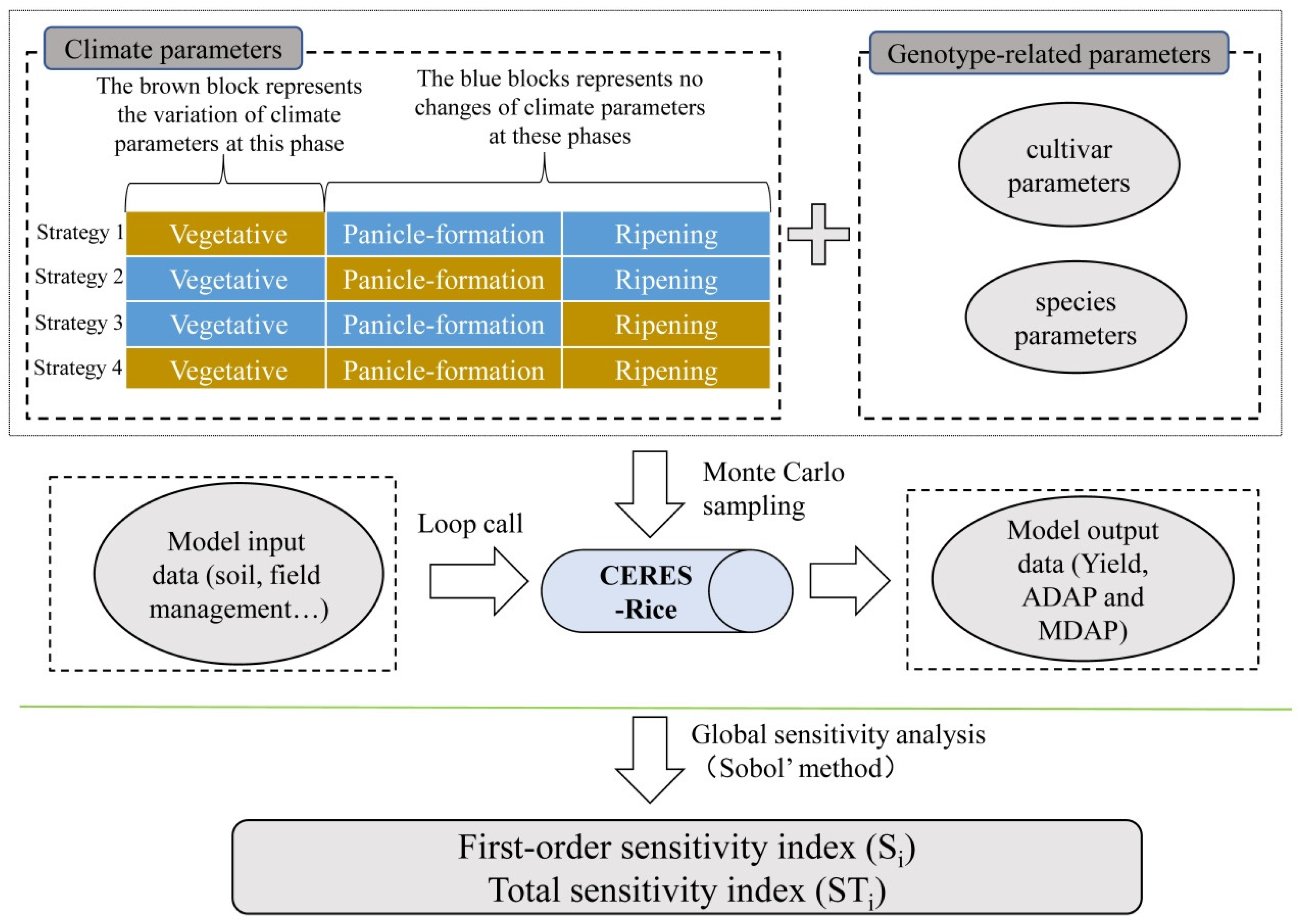
2.3.2. Crop Modeling

To run the CERES-Rice model, parameters and inputs including weather data, soil profile information, field management data, and genotype parameter data were required. The minimum requirements of weather data contained daily minimum and maximum temperature, daily rainfall, and daily solar radiation. These data were collected from the local weather station. The soil profile data is listed in Table 1. Field management data are introduced in Section 2.1. In the CERES-Rice model, the genotype parameters included cultivar, species, and ecotype coefficients. There were eight cultivar coefficients which were used to describe the hereditary characteristics of the specific genotypes. Among them, four cultivar parameters (P1, P2R, P5, P2O) were related to phenology and another four parameters (G1, G2, G3 and G4) were pertinent to rice growth and development. The species coefficients were set as default values. At present, the ecotype coefficients are not available for common users in the CERES-Rice model. Accordingly, only eight cultivar parameters were determined in this study.

The time period (growing degree days, °C$·$d) from beginning of grain filling (3–4 days after flowering) to physiological maturity (P5) was calculated based on observation data. Single grain weight (G2) was set based on 1000-grain weight. The calculation of cultivar parameters based on observed data in DSSAT has been described by Yan et al. [40]. The specific calculation processes of P5 and G2 were as follows:

$$\mathrm{P}5={\displaystyle \sum }_i^m\left(Tav{g}_i-T_{base}\right)\{\begin{array}{c}Tav{g}_i=(Tma{x}_i+Tmi{n}_{\mathrm{i}})/2 \\ Tav{g}_i=T_{base} if Tav{g}_i\le T_{base}\\ Tav{g}_i=T_{upper} if Tav{g}_i\ge T_{upper}\end{array}$$

(1)

$$\mathrm{G}2=W/1000$$

(2)

where $i$= 1, 2, … $m$ days between beginning of grain filling and physiological maturity. On the $i_{th}$ day, $Tav{g}_i$ is the daily average temperature (°C); $Tmi{n}_i$ is the daily minimum temperature (°C); $Tma{x}_i$ is the daily maximum temperature (°C); $T_{base}$ is the base temperature of 9 °C; $T_{upper}$ is set to 40 °C. In equation 2, $\mathrm{W}$ represents the 1000-grain weight (g).

Other six parameters (P1, P2R, P2O, G1, G3 and G4) of each rice cultivar were determined by the Generalized Likelihood Uncertainty Estimation (GLUE) method which has been widely used in model calibration [41,42]. The specific procedures of the GLUE method are mainly as follows [15,43]:

(1)

Set parameter range by using the default range (

Table A1. Cultivar parameters range of the CERES-Rice model.

Parameter	Description	Unit	Range
P1	Time period in °C above a base temperature of 9 °C during the basic vegetative phase	GDD (°C)	210–900
P2O	Critical photoperiod (in hours) at which the development occurs at a maximum rate	hours	10.4–13
P2R	Extent to which phasic development leading to panicle initiation is delayed for each hour increase in photoperiod above P2O	GDD h−1	30–200
G1	Potential spikelet number coefficient	--	50–80
G3	Tillering coefficient relative to IR64 cultivar under ideal conditions	--	0.3–1
G4	Temperature tolerance coefficient	--	0.8–1.25

) in the CERES-Rice model. Uniform parameter distributions were assumed to generate parameter sets. In this study, 10,000 parameter sets were randomly generated by Python 3.6.

(2)

Select the observation data including anthesis date, maturity date, and grain yield as our objectives.

(3)

Run the CERES-Rice model. The executable file “DSCSM047.exe” was looped called Python 3.6 based on the abovementioned parameter sets.

(4)

Calculate the likelihood value. A likelihood function which was described by He et al. [41] was implemented to obtain likelihood values based on simulations and observations.

(5)

Calculate the cultivar parameters based on the maximum likelihood value.

2.4. Sensitivity Analysis

2.4.1. Sobol’ Method

In this study, the Sobol’ algorithm was implemented to rank sensitivity of input parameters or variables to the model outputs (ADAP, MDAP and yield). The Sobol’ global SA calculates the analysis of variance-based decomposition of output variance, where the main effects and interaction terms can be computed [44]. The Sobol’ sensitivity index is the fraction of total variance which is attributed to any individual factor or combination of factors [45]. In addition, the Sobol’ method can calculate the total sensitivity index ($S{T}_i$), defined as the sum of the first-order and higher-order effects involving all the input factors. With $\mathrm{m}$ quantitative input factors, the decomposition of variance $\mathrm{var}\left(\mathrm{Y}\right)$ can be calculated as follow:

$$\mathrm{var}\left(\mathrm{Y}\right)={\displaystyle \sum }_{\mathrm{i}=1}^{\mathrm{m}}{\mathrm{v}}_{\mathrm{i}}+{\displaystyle \sum }_{1\le \mathrm{i}<\mathrm{j}\le \mathrm{m}}{\mathrm{v}}_{\mathrm{ij}}+\cdots +{\mathrm{v}}_{1,2,\dots ,\mathrm{m}}$$

(3)

where ${\mathrm{v}}_{\mathrm{i}}$ is the variability based on the main effect of input factor ${\mathrm{x}}_{\mathrm{i}}$; ${\mathrm{v}}_{\mathrm{ij}}$ is the variability based on the interaction effect between input factors (${\mathrm{x}}_{\mathrm{i}}$ and ${\mathrm{x}}_{\mathrm{j}}$); ${\mathrm{v}}_{1,2,\dots ,\mathrm{m}}$ is the variability based on the interaction effect between all input factors (${\mathrm{x}}_1,{\mathrm{x}}_2,\dots ,{\mathrm{x}}_{\mathrm{m}}$). $\mathrm{var}\left(\mathrm{Y}\right)$ represents the variability of $\mathrm{Y}$ including the overall uncertainty of the input factors. The sensitivity indices are calculated from Equation (3) by dividing the individual importance measures by the total variance $\mathrm{var}\left(\mathrm{Y}\right)$.

$${\mathrm{S}}_{\mathrm{i}}=\frac{{\mathrm{v}}_{\mathrm{i}}}{\mathrm{var}\left(\mathrm{Y}\right)}$$

(4)

$${\mathrm{SI}}_{\mathrm{ij}}=\frac{{\mathrm{v}}_{\mathrm{ij}}}{\mathrm{var}\left(\mathrm{Y}\right)}$$

(5)

where ${\mathrm{S}}_{\mathrm{i}}$ is defined as the first order sensitivity index of input factor ${\mathrm{x}}_{\mathrm{i}}$, representing the main effect of factor ${\mathrm{x}}_{\mathrm{i}}$ on the output. ${\mathrm{SI}}_{\mathrm{ij}}$ is defined as the second-order sensitivity index which represents the interaction effect of two factors ${\mathrm{x}}_{\mathrm{i}}$ and ${\mathrm{x}}_{\mathrm{j}}$.

Sobol’ input samples were generated by using the Python library “SALib” and executed by a size of $\mathrm{m}\left(2\mathrm{n}+2\right)$ model input sets in Python 3.6, where $\mathrm{m}$ required a range of 100 or larger [44]. Sixteen parameters ($\mathrm{n}$) were selected to implement global SA (

Table 3. Description of the 16 investigated parameters in the CERES-Rice model.

Type	Parameter	Description	Unit	Range
Cultivar parameter	P1	Time period in °C above a base temperature of 9 °C during the basic vegetative phase.	GDD (°C)	$\pm 30\%$
	P2O	Critical photoperiod (in hours) at which the development occurs at a maximum rate.	hours	$\pm 30\%$
	P2R	Extent to which phasic development leading to panicle initiation is delayed for each hour increase in photoperiod above P2O	GDD h−1	$\pm 30\%$
	P5	Time period in °C above a base temperature of 9 °C from beginning of grain filling (3–4 days after anthesis) to physiological maturity.	GDD (°C)	$\pm 30\%$
	G1	Potential spikelet number coefficient	--	$\pm 30\%$
	G2	Single grain weight (g) under ideal growing conditions	g	$\pm 30\%$
	G3	Tillering coefficient relative to IR64 cultivar under ideal conditions.	--	$\pm 30\%$
	G4	Temperature tolerance coefficient.	--	$\pm 30\%$
Species parameter	SHFC	Shock calculation method (1-standard, 2-Salaam)	--	$\pm 30\%$
	RWEP	Species coefficient	--	$\pm 30\%$
	PORM	Minimum pore space	--	0–0.3
	RWMX	Max root water uptake	--	$\pm 30\%$
	RLWR	Root length weight ratio	--	$\pm 30\%$
Climate parameter	SRAD	Daily solar radiation	MJ m−2 day−1	$\pm 30\%$
	Tavg	Daily average temperature	°C	$\pm 30\%$
	RAIN	Daily rainfall	mm day−1	$\pm 30\%$

). In this study, we used $\mathrm{m}=3$50 and $\mathrm{n}=1$6 for a total of 11,900 input parameter sets for each cultivar. Four specific-stage variations of climate parameters were considered (Figure 1). The investigated stages include the whole growth season, vegetative phase, panicle-formation phase and ripening phase. Accordingly, the total number of model executions was 30$\times$11,900$\times$4 = 1,428,000. The majority of global SA computations described in this paper were performed on the High-Performance Computing System at the Institute of Soil Science, Chinese Academy of Sciences.

2.4.2. Top-Down Concordance Coefficient ($TDCC$)

The top-down concordance coefficient ($TDCC$) can quantify agreements among multiple rankings. The $TDCC$ adopts the savage scoring method to emphasize the consistency of influential parameter rankings and to de-emphasize the inconsistency of non-influential parameter rankings [46]. The $TDCC$ was calculated using the following equation:

$$S_{ij}={\displaystyle \sum }_{i=r_{ij}}^n\raisebox{1ex}{$1$}\!\left/ \!\raisebox{-1ex}{$i$}\right.$$

(6)

$$TDCC=\frac{{\sum }_{i=1}^n{\left({\sum }_{j=1}^m{S}_{ij}\right)}^2-m^{2}n}{m^2\left(n-{\sum }_{i=1}^n\raisebox{1ex}{$1$}\!\left/ \!\raisebox{-1ex}{$i$}\right.\right)}$$

(7)

where $S_{ij}$ is the savage score of the $i_{th}$ parameter in the $j_{th}$ SA experiment; $r_{ij}$ is the rank of the $i_{th}$ parameter in the $j_{th}$ SA experiment; $n$ is the number of investigated parameters; and $m$ is the number of SA objectives.

The p-value was calculated to test the $TDCC$’s significance, which is calculated as follows:

$$T=m\left(n-1\right)TDCC$$

(8)

where $T$ is close to the chi-squared distribution with $n-1$ degrees of freedom. In general, rankings were considered statistically consistent if the p-value derived from $TDCC$ was smaller than 0.05.

3. Results

3.1. Distribution of Observation Data across Different Cultivars

The distributions of observations including dates of anthesis and maturity, and grain yield are presented in

Table 4. Distributions of anthesis and maturity dates, and grain yield among mid-season, late-season, and one-season-late rice cultivars in 2018.

Observation Index	Cultivar Type	Number of Cultivars	Statistical Indicators
			Mean	Median	25th Percentile	75th Percentile
Anthesis date	Mid-season	12	8-August	8-August	7-August	9-August
	Late-season	9	3-September	2-September	1-September	4-September
	One-season-late	9	29-August	30-August	26-August	30-August
Maturity date	Mid-season	12	12-September	13-September	10-September	14-September
	Late-season	9	20-October	19-October	18-October	21-October
	One-season-late	9	11-October	12-October	11-October	12-October
Yield (t ha−1)	Mid-season	12	9.7	9.6	9.4	10.1
	Late-season	9	8.2	7.8	8.0	8.5
	One-season-late	9	9.9	9.7	9.6	10.1

. Among different cultivar types, the mid-season rice had the earliest date of anthesis. Although, the sowing date for late-season cultivars was two weeks later than that for one-season-late cultivars, the anthesis dates for these two cultivar types were close. The mean anthesis dates were 8 August, 3 September, and 29 August for mid-season, late-season, and one-season-late rice cultivar types, respectively in 2018. As for physiological maturity, all the mid-season rice cultivars were harvested in September, and all late-season and one-season-late rice cultivars were harvested in October. The mean maturity dates for mid-season, late-season, and one-late-season rice cultivars were 12 September, 20 October, and 11 October, respectively. Additionally, the yield of one-season-late cultivars tended to be slight larger than that of mid-season cultivars; the yield obtained from late-season cultivars was the lowest.

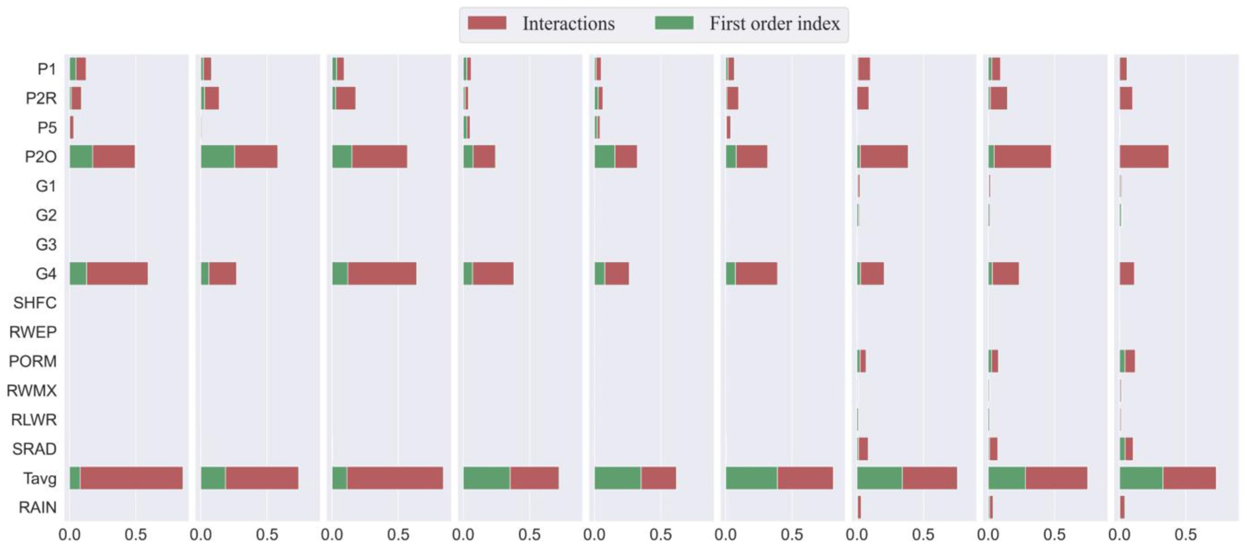
3.2. Sensitivity Analysis during the Rice Growth Season

For both ADAP and MDAP, parameters P2O, G4, Tavg were more influential than other parameters among different cultivar types (Figure 2). G4 in late-season and mid-season cultivars showed larger inter-cultivar variability than that in one-season-late cultivars. Tavg had the largest influence on $S{T}_i$ values for phenology in all cultivars. For yield, parameters Tavg and P2O had a markedly larger influence and inter-cultivar variability. The variations of $S{T}_i$ values were similar in different cultivar types. In general, the more influential parameters (Tavg and P2O) showed a more evident difference between cultivars.

Figure 3 shows the mean $S_i$ values and interactions between parameters under different cultivar types when the variation of climate parameters occurred for the whole growth season. Different cultivar types demonstrated similar effects on the sensitivity results of the investigated parameters for ADAP, MDAP, and yield; for instance, the most influential parameters (Tavg, P2O, G4) were the same. It is worth mentioning that the influence of the interaction among parameters on all outputs of the CERES-Rice model was notable. For ADAP, the interaction indices of Tavg, P2O, and G4 contributed to 64.9–90.7%, 56.1–77.4%, and 73.5–86.6%, respectively in late-season, one-season-late, and mid-season cultivar types. For MDAP, though the most influential parameters were the same as those for ADAP, the interaction effects of these parameters were slightly smaller and contributed to 51.2–81.7%, 43.0–70.2%, and 51.9–81.5%, respectively in late-season, one-season-late, and mid-season cultivar types. For yield, the interaction effects of cultivar parameters contributed approximately 90% such as P1, P2R, P2O, and G4. The climate parameter Tavg contributed 54.8%, 62.5%, and 55.2% for the variance of yield, respectively in late-season, one-season-late, and mid-season cultivar types.

Table 5. $TDCC$ values based on the results of Sobol’ total order effects ($S{T}_i$ ) under the same cultivar type and different cultivar types over the whole growth season.

Model Output	Same Cultivar Type			Different Cultivar Types
	Late-Season	One-Season-Late	Mid-Season	L-O	L-M	O-M
ADAP	0.95	0.98	0.94	0.99	0.99	0.99
MDAP	0.98	0.96	0.98	0.98	0.98	0.98
Yield	0.98	0.99	0.97	1.00	1.00	1.00

Note: L-O rice represents the cultivars between late-season and one-season-late cultivar types; L-M rice represents the cultivars between late-season and mid-season cultivar types; O-M rice represents the cultivars between one-season-late and mid-season cultivar types.

shows the values of $TDCC$ under the different cultivar types. The different cultivars in the same cultivar type had no noticeable effect on the parameter ranking for the model outputs. The $TDCC$ values were larger than 0.93 for all output variables. Additionally, the $TDCC$ values in different cultivar types were greater than 0.98 for all output variables. The corresponding p-values are not presented in this study but were less than 0.05. In general, different cultivars had no statistical influence on the rankings of the sensitivity parameters.

3.3. Sensitivity Analysis under Specific-Stage Variations of Climate Parameters

3.3.1. Sensitivity Analysis under the Variation of Climate Parameters at the Vegetative Phase

Figure 4 illustrates the mean $S_i$ values and interactions between parameters under different cultivar types when the variation of climate parameters occurs at the vegetative phase. At this stage, the effects of P2O ($S_i$ ranged from 0.61 to 0.70) and Tavg ($S_i$ ranged from 0.12 to 0.25) on model outputs (ADAP and MDAP) were significant, while the interactions between parameters were non-significant. Except for P2O and Tavg, the species parameter PORM showed a notable effect on yield ($S{T}_i$ > 0.05). Different cultivar types indicated no differences in the sensitivity results of the investigated parameters for ADAP, MDAP, and Yield. Parameter P2O was the most sensitive for all model outputs, whereas the growth-related parameters (e.g., G1, G2, G3, and G4) showed negligible effects on the model outputs ($S{T}_i$ < 0.05). The sensitivity rankings of the 16 investigated parameters were statistically consistent among different cultivars (

Table 6. $TDCC$ values based on the results of Sobol’ total order effects ($S{T}_i$ ) under the same cultivar type and different cultivar types with variation of climate parameters at the vegetative phase.

Model Output	Same Cultivar Type			Different Cultivar Types
	Late-Season	One-Season-Late	Mid-Season	L-O	L-M	O-M
ADAP	0.98	0.99	0.98	1.00	1.00	1.00
MDAP	0.98	0.97	0.95	0.99	0.98	0.98
Yield	0.96	0.97	0.99	0.99	0.97	0.97

Note: L-O rice represents the cultivars between late-season and one-season-late cultivar types; L-M rice represents the cultivars between late-season and mid-season cultivar types; O-M rice represents the cultivars between one-season-late and mid-season cultivar types.

).

3.3.2. Sensitivity Analysis under Variation of Climate Parameters at the Panicle-Formation Phase

Figure 5 presents the sensitivity indices of the 16 investigated parameters for model outputs simulated in late-season, one-season-late, and mid-season rice cultivar types, respectively under the panicle-formation-phase variation of climate parameters. At this stage, climate parameters (SRAD, Tavg, and RAIN) had no influence on the variations of all model outputs; the $S{T}_i$ values were less than 0.05. For ADAP and MDAP, only phenology-related parameters (P1, P2R, P5, and P2O) had a notable influence on the model outputs. For yield, parameter P2O ($S{T}_i$ > 0.70) was the most sensitive parameter, followed by PORM ($S{T}_i$ > 0.10). The growth-related parameters (G1 and G2) indicated slight effects on yield. In general, the effects of single parameters ($S_i$) on model outputs were significant, while interactions between parameters were non-significant. In addition, the sensitivity rankings of parameters were statistically consistent among various cultivars (

Table 7. $TDCC$ values based on the results of Sobol’ total order effects ($S{T}_i$ ) under the same cultivar type and different cultivar types with variation of climate parameters at the panicle-formation phase.

Model Output	Same Cultivar Type			Different Cultivar Types
	Late-Season	One-Season-Late	Mid-Season	L-O	L-M	O-M
ADAP	0.99	0.99	0.99	0.99	0.99	0.99
MDAP	0.96	0.96	0.97	0.96	0.96	0.96
Yield	0.96	0.98	0.97	0.98	0.98	0.98

Note: L-O rice represents the cultivars between late-season and one-season-late cultivar types; L-M rice represents the cultivars between late-season and mid-season cultivar types; O-M rice represents the cultivars between one-season-late and mid-season cultivar types.

).

3.3.3. Sensitivity Analysis under Variation of Climate Parameters at the Ripening Phase

Figure 6 shows the mean sensitivity indices of the 16 investigated parameters under the ripening-phase variation of climate parameters, simulated on late-season, one-season-late, and mid-season rice cultivar types, respectively. For ADAP, the cultivar types showed no significant influence on the ranks of parameter sensitivities. Parameter P2O was the most influential parameter for ADAP ($S{T}_i$ > 0.82). Except for phenology-related parameters (P2, P2R and P2O), other parameters demonstrated no effect on the variation of ADAP ($S{T}_i$ < 0.05). For MDAP, parameter Tavg indicated more effects on MDAP in the late-season cultivar type than in the one-season cultivar type. However, Tavg in the mid-season cultivar type showed negligible effects on the variability of MDAP ($S{T}_i$ < 0.05). For yield, parameter P2O and PORM were the most sensitive parameters. The growth-related parameters (G1 and G2) had minor effects on yield. The effects of interactions between parameters on the model outputs were non-significant.

Table 8. $TDCC$ values based on the results of Sobol’ total order effects ($S{T}_i$ ) under the same cultivar type and different cultivar types with variation of climate parameters at the ripening phase.

Model Output	Same Cultivar Type			Different Cultivar Types
	Late-Season	One-Season-Late	Mid-Season	L-O	L-M	O-M
ADAP	0.99	1.00	0.99	0.99	0.99	0.99
MDAP	0.96	0.97	0.97	0.96	0.95	0.95
Yield	0.97	0.98	0.98	0.99	0.98	0.98

Note: L-O rice represents the cultivars between late-season and one-season-late cultivar types; L-M rice represents the cultivars between late-season and mid-season cultivar types; O-M rice represents the cultivars between one-season-late and mid-season cultivar types.

shows that the $TDCC$ values among different rice cultivars were above 0.95.

4. Discussion

4.1. Sensitivity Analysis of Different Cultivars for Model Outputs during the Rice Growth Season

Crop growth models become more complicated due to the improvements in the understanding of the physiological and ecological processes and their interactions and the increased computing power of the corresponding simulators with several related parameters to estimate. Global SA is an important component of modelling practices which could help in factor prioritization [47], and the Sobol’ method demonstrated the sensitivity of the CERES-Rice model with a variety of 16 investigated parameters among 30 rice cultivars for ADAP, MDAP, and yield during the rice growth season. Although, only one year of data was used to analyze the SA of the experiment area, it has been reported that data from one year or a single growth season can be used for the global SA [16,33]. Besides, the sensitivity ranking of the parameters was not significantly affected by the year [48]. The computationally expensive Sobol’ SA method helped us to understand the overall functioning of the CERES-Rice model in cultivar variations of the breeding trials and then to implement a quantitative evaluation of SA for the model outputs. Although, variance-based methods have expensive computation cost, they can explore all regions of input space and consider both interaction and nonlinear response [21,49].

For different cultivars, the $TDCC$ values for all model outputs were more than 0.90 (Table 5); this indicated that the effects of cultivars on parameter rankings were not significant (p < 0.05), which is due to two reasons: (1) different cultivars in the breeding trials showed similar phenotypic traits (Table 4) and (2) these genotypes were all obtained from two parents in this study. In addition, the cultivar types (e.g., late-season, one-season-late, and mid-season types) had little effect on the ranking of the influential parameters for model outputs. However, due to the variation of growth duration length, the distribution of sensitivity index values of inter-cultivars was slightly inconsistent in the different cultivar types (Figure 2).

As for specifically influential parameters, the Tavg, G4, and P2O ($S{T}_i$ > 0.24) were the most sensitive parameters for the variation of ADAP and MDAP. In the CERES-Rice model, the development rate of rice depended on the degree days (DD). Parameter Tavg which determined the daily maximum and minimum temperature was a key factor in calculating the day’s value of DD [50]. Accordingly, parameter Tavg ($S{T}_i$ > 0.61) was the most influential parameter for rice phenology among all cultivars. Parameter G4 was the temperature tolerance coefficient, the influences of parameter interactions were greater than the influences of the first-order contribution (Figure 3). Parameter P2O represented the longest day length when the development rate was maximum. Compared to other phenology-related parameters (P1, P2R, and P5), parameter P2O was more sensitive to phenology, which was mainly because the longest day length in the breeding site was larger than P2O; thus, a notable effect on the results. For yield, the most sensitive parameters were similar to those for ADAP and MDAP (Figure 3), which could be explained by the close relationship between growth duration length and panicle formation. It was of note that the species parameter PORM (minimum pore space) had considerable influence on yield. All the $S{T}_i$ values of PORM among different cultivars were larger than 0.05.

4.2. Effects of Specific-Stage Variations of Climate Parameters on Sensitivity

This study demonstrated a new comprehensive insight into the SA of a crop model with variations of climate parameters at specific stages. The variation of climate parameters was divided into three phases: (1) vegetative phase (sowing to initial heading), (2) panicle-formation phase (initial heading to full heading), and (3) ripening phase (full heading to maturity). When the variation of climate parameters occurred at the vegetative phase, Tavg showed significant effects on the model outputs. It demonstrated that the rice growth was easily affected by the changes of climate conditions at the vegetative phase regardless of the different cultivars (Figure 4). In phenology-related parameters, P2O was the most sensitive parameter for the model outputs. The result agreed with the global SA when the variation of climate parameters occurred during the whole growth season (Figure 7). At panicle-formation phase, climate parameters indicated no effects on the model outputs, which was likely due to the small duration length of this phase (4–5 days) which had negligible influence on the accumulation of degree days. At the ripening phase, climate parameters showed no influence on ADAP (Figure 6), which was because ADAP was only controlled by the accumulation of thermal time from planting to flowering. The effects of climate parameters on different cultivar types were not completely concordant. For instance, parameter Tavg in late-season and one-season-late cultivars showed a considerable effect on MDAP ($S{T}_i$ > 0.1); while Tavg in mid-season cultivars indicated no significant effect on MDAP ($S{T}_i$ < 0.05). In general, the sensitivity rankings of the parameters were similar under variations of climate parameters at the panicle-formation phase and ripening phase (Figure 5, Figure 6 and Figure 7).

Cultivars with environment studies have been conducted such as investigations of ideal cultivars for the given environments for rice [51] and wheat [52], as well as investigations of genetic gains in soybean for given possible sources [53]. However, due to the variation of irrigation, fertilization, and soil conditions, these factors could bring large uncertainty as well as interactions for the global SA. In this study, all the investigated cultivars were planted in the same site with the same field management and soil conditions; we only analyzed the effects of inter-cultivars and cultivar types for the model outputs with variation of climate parameters at specific stages, which allowed for testing the CERES-Rice model responses to the changes of cultivars and climate status as well as utilizing genotypes in the currently explored conditions in the breeding trials. The ideal cultivars in different locations might be related to different climate conditions. Therefore, the variations of climate conditions at specific phases should be considered in selecting reasonable cultivar types in rice breeding.

5. Conclusions

The Sobol’ method was applied to investigate the effects of cultivars and different specific-stage variations of climate parameters on parameter sensitivity in the CERES-Rice model. The global SA demonstrated that the variation of climate parameters was: (1) for the whole rice growth season, the interactions between parameters were larger than the effects of the parameters themselves for the model outputs and different cultivar types showed no significant effects on parameter rankings (p < 0.05); (2) at the vegetative phase, Tavg indicated a considerable effect on the variation of all the model outputs; (3) at the panicle-formation phase, the climate parameters demonstrated no effect on model outputs ($S{T}_i$ < 0.05); (4) and at the ripening phase, ADAP were only affected by phenology-related parameters while Tavg showed different effects on MDAP depending on the cultivar types. Additionally, the species parameter PORM indicated an indispensable influence on yield regardless of the different specific-stage variations of the climate conditions ($S{T}_i$ > 0.05). In all, these investigations provided useful knowledge to guide efforts toward model calibration and applications in rice breeding trials.

References

1. Fang, Q.X.; Malone, R.W.; Ma, L.; Jaynes, D.B.; Thorp, K.R.; Green, T.R.; Ahuja, L.R. Modeling the effects of controlled drainage, N rate and weather on nitrate loss to subsurface drainage. Agric. Water Manag. 2012, 103, 150–161. [Google Scholar] [CrossRef]
2. Wu, L.; Liu, X.; Wang, P.; Zhou, B.; Liu, M.; Li, X. The assimilation of spectral sensing and the WOFOST model for the dynamic simulation of cadmium accumulation in rice tissues. Int. J. Appl. Earth Obs. Geoinf. 2013, 25, 66–75. [Google Scholar] [CrossRef]
3. Holzkaemper, A.; Calanca, P.; Honti, M.; Fuhrer, J. Projecting climate change impacts on grain maize based on three different crop model approaches. Agric. For. Meteorol. 2015, 214, 219–230. [Google Scholar] [CrossRef]
4. Li, T.; Raman, A.K.; Marcaida, M., III; Kumar, A.; Angeles, O.; Radanielson, A.M. Simulation of genotype performances across a larger number of environments for rice breeding using ORYZA2000. Field Crops Res. 2013, 149, 312–321. [Google Scholar] [CrossRef]
5. Jones, J.W.; Hoogenboom, G.; Porter, C.H.; Boote, K.J.; Batchelor, W.D.; Hunt, L.A.; Wilkens, P.W.; Singh, U.; Gijsman, A.J.; Ritchie, J.T. The DSSAT cropping system model. Eur. J. Agron. 2003, 18, 235–265. [Google Scholar] [CrossRef]
6. Santangelo, G.; Bramanti, L.; Iannelli, M. Population dynamics and conservation biology of the over-exploited Mediterranean red coral. J. Theor. Biol. 2007, 244, 416–423. [Google Scholar] [CrossRef]
7. Liang, H.; Qi, Z.; DeJonge, K.C.; Hu, K.; Li, B. Global sensitivity and uncertainty analysis of nitrate leaching and crop yield simulation under different water and nitrogen management practices. Comput. Electron. Agric. 2017, 142, 201–210. [Google Scholar] [CrossRef]
8. Tan, J.; Cui, Y.; Luo, Y. Global sensitivity analysis of outputs over rice-growth process in ORYZA model. Environ. Model. Softw. 2016, 83, 36–46. [Google Scholar] [CrossRef]
9. Confalonieri, R.; Bellocchi, G.; Bregaglio, S.; Donatelli, M.; Acutis, M. Comparison of sensitivity analysis techniques: A case study with the rice model WARM. Ecol. Model. 2010, 221, 1897–1906. [Google Scholar] [CrossRef]
10. Lamboni, M.; Makowski, D.; Lehuger, S.; Gabrielle, B.; Monod, H. Multivariate global sensitivity analysis for dynamic crop models. Field Crops Res. 2009, 113, 312–320. [Google Scholar] [CrossRef]
11. Cariboni, J.; Gatelli, D.; Liska, R.; Saltelli, A. The role of sensitivity analysis in ecological modelling. Ecol. Model. 2007, 203, 167–182. [Google Scholar] [CrossRef]
12. Vanuytrecht, E.; Raes, D.; Willems, P. Global sensitivity analysis of yield output from the water productivity model. Environ. Model. Softw. 2014, 51, 323–332. [Google Scholar] [CrossRef] [Green Version]
13. van Griensven, A.; Meixner, T.; Grunwald, S.; Bishop, T.; Diluzio, A.; Srinivasan, R. A global sensitivity analysis tool for the parameters of multi-variable catchment models. J. Hydrol. 2006, 324, 10–23. [Google Scholar] [CrossRef]
14. Wang, J.; Li, X.; Lu, L.; Fang, F. Parameter sensitivity analysis of crop growth models based on the extended Fourier Amplitude Sensitivity Test method. Environ. Model. Softw. 2013, 48, 171–182. [Google Scholar] [CrossRef]
15. Jha, P.K.; Ines, A.; Singh, M.P. A multiple and ensembling approach for calibration and evaluation of genetic coefficients of CERES-Maize to simulate maize phenology and yield in Michigan. Environ. Model. Softw. 2021, 135, 104901. [Google Scholar] [CrossRef]
16. Jin, X.; Li, Z.; Nie, C.; Xu, X.; Feng, H.; Guo, W.; Wang, J. Parameter sensitivity analysis of the AquaCrop model based on extended fourier amplitude sensitivity under different agro-meteorological conditions and application. Field Crops Res. 2018, 226, 1–15. [Google Scholar] [CrossRef]
17. Saltelli, A.; Ratto, M.; Tarantola, S.; Campolongo, F. Sensitivity analysis practices: Strategies for model-based inference. Reliab. Eng. Syst. Saf. 2006, 91, 1109–1125. [Google Scholar] [CrossRef]
18. Wu, M.; Ran, Y.; Jansson, P.-E.; Chen, P.; Tan, X.; Zhang, W. Global parameters sensitivity analysis of modeling water, energy and carbon exchange of an arid agricultural ecosystem. Agric. For. Meteorol. 2019, 271, 295–306. [Google Scholar] [CrossRef]
19. Morris, M.D. Factorial sampling plans for preliminary computational experiments. Technometrics 1991, 33, 161–174. [Google Scholar] [CrossRef]
20. Cukier, R.I.; Schaibly, J.H.; Shuler, K.E. Study of the sensitivity of coupled reaction systems to uncertainties in rate coefficients. III. Analysis of the approximations. J. Chem. Phys. 1975, 63, 1140–1149. [Google Scholar] [CrossRef]
21. Nossent, J.; Elsen, P.; Bauwens, W. Sobol’ sensitivity analysis of a complex environmental model. Environ. Model. Softw. 2011, 26, 1515–1525. [Google Scholar] [CrossRef]
22. Varella, H.; Guerif, M.; Buis, S. Global sensitivity analysis measures the quality of parameter estimation: The case of soil parameters and a crop model. Environ. Model. Softw. 2010, 25, 310–319. [Google Scholar] [CrossRef]
23. Jawitz, B.; Muñoz-Carpena, R.; Muller, S.; Grace, K.A.; James, A. Development, Testing, and Sensitivity and Uncertainty Analyses of a Transport and Reaction Simulation Engine (TaRSE) for Spatially Distributed Modeling of Phosphorus in the Peat Marsh Wetlands of Southern Florida: U.S. Geological Survey Scientific Investigations Report 2008-5029, 109 p. Available online: https://pubs.usgs.gov/sir/2008/5029/ (accessed on 20 November 2021).
24. Tang, Y.; Reed, P.; van Werkhoven, K.; Wagener, T. Advancing the identification and evaluation of distributed rainfall-runoff models using global sensitivity analysis. Water Resour. Res. 2007, 43, W06415. [Google Scholar] [CrossRef]
25. Ziehn, T.; Tomlin, A.S. Global sensitivity analysis of a 3D street canyon model—Part I: The development of high dimensional model representations. Atmos. Environ. 2008, 42, 1857–1873. [Google Scholar] [CrossRef]
26. Meszaros, R.; Zsely, I.G.; Szinyei, D.; Vincze, C.; Lagzi, I. Sensitivity analysis of an ozone deposition model. Atmos. Environ. 2009, 43, 663–672. [Google Scholar] [CrossRef]
27. Confalonieri, R. Monte Carlo based sensitivity analysis of two crop simulators and considerations on model balance. Eur. J. Agron. 2010, 33, 89–93. [Google Scholar] [CrossRef]
28. Lo-Pelzer, E.; Bousset, L.; Jeuffroy, M.H.; Salam, M.U.; Pinochet, X.; Boillot, M.; Aubertot, J.N. SIPPOM-WOSR: A Simulator for Integrated Pathogen POpulation Management of phoma stem canker on Winter OilSeed Rape I. Description of the model. Field Crops Res. 2010, 118, 73–81. [Google Scholar] [CrossRef]
29. Stella, T.; Frasso, N.; Negrini, G.; Bregaglio, S.; Cappelli, G.; Acutis, M.; Confalonieri, R. Model simplification and development via reuse, sensitivity analysis and composition: A case study in crop modelling. Environ. Model. Softw. 2014, 59, 44–58. [Google Scholar] [CrossRef]
30. Wang, X.; He, X.; Williams, J.R.; Izaurralde, R.C.; Atwood, J.D. Sensitivity and uncertainty analyses of crop yields and soil organic carbon simulated with EPIC. Trans. ASAE 2005, 48, 1041–1054. [Google Scholar] [CrossRef]
31. Confalonieri, R.; Bellocchi, G.; Tarantola, S.; Acutis, M.; Donatelli, M.; Genovese, G. Sensitivity analysis of the rice model WARM in Europe: Exploring the effects of different locations, climates and methods of analysis on model sensitivity to crop parameters. Environ. Model. Softw. 2010, 25, 479–488. [Google Scholar] [CrossRef]
32. de Almeida Pereira, R.A.; Vianna, M.d.S.; Pinto Nassif, D.S.; Carvalho, K.d.S.; Marin, F.R. Global sensitivity and uncertainty analysis of a sugarcane model considering the trash blanket effect. Eur. J. Agron. 2021, 130, 126371. [Google Scholar] [CrossRef]
33. Tan, J.; Cui, Y.; Luo, Y. Assessment of uncertainty and sensitivity analyses for ORYZA model under different ranges of parameter variation. Eur. J. Agron. 2017, 91, 54–62. [Google Scholar] [CrossRef]
34. Liu, J.; Liu, Z.; Zhu, A.X.; Shen, F.; Lei, Q.; Duan, Z. Global sensitivity analysis of the APSIM-Oryza rice growth model under different environmental conditions. Sci. Total Environ. 2019, 651, 953–968. [Google Scholar] [CrossRef] [Green Version]
35. Yang, Q.; Shi, L.; Han, J.; Yu, J.; Huang, K. A near real-time deep learning approach for detecting rice phenology based on UAV images. Agric. For. Meteorol. 2020, 287, 107938. [Google Scholar] [CrossRef]
36. Fageria, N.K. Yield physiology of rice. J. Plant Nutr. 2007, 30, 843–879. [Google Scholar] [CrossRef]
37. Nicolas, F.; Migliaccio, K.W.; Hoogenboom, G.; Rathinasabapathi, B.R.; Eisenstadt, W.R. Assessing the potential impact of climate change on rice yield in the Artibonite Valley of Haiti using the CSM-CERES-Rice model. Trans. ASABE 2020, 63, 1385–1400. [Google Scholar] [CrossRef]
38. Alejo, L.A. Assessing the impacts of climate change on aerobic rice production using the DSSAT-CERES-Rice model. J. Water Clim. Chang. 2021, 12, 696–708. [Google Scholar] [CrossRef]
39. Zhang, J.; Miao, Y.; Batchelor, W.D.; Lu, J.; Wang, H.; Kang, S. Improving High-Latitude Rice Nitrogen Management with the CERES-Rice Crop Model. Agronomy 2018, 8, 263. [Google Scholar] [CrossRef] [Green Version]
40. Yan, L.; Jin, J.; Wu, P. Impact of parameter uncertainty and water stress parameterization on wheat growth simulations using CERES-Wheat with GLUE. Agric. Syst. 2020, 181, 102823. [Google Scholar] [CrossRef]
41. He, J.; Jones, J.W.; Graham, W.D.; Dukes, M.D. Influence of likelihood function choice for estimating crop model parameters using the generalized likelihood uncertainty estimation method. Agric. Syst. 2010, 103, 256–264. [Google Scholar] [CrossRef]
42. Sexton, J.; Everingham, Y.; Inman-Bamber, G. A theoretical and real world evaluation of two Bayesian techniques for the calibration of variety parameters in a sugarcane crop model. Environ. Model. Softw. 2016, 83, 126–142. [Google Scholar] [CrossRef]
43. Memic, E.; Graeff, S.; Boote, K.J.; Hensel, O.; Hoogenboom, G. Cultivar coefficient estimator for the cropping system model based on time-series data: A case study for soybean. Trans. ASABE 2021, 64, 1391–1402. [Google Scholar] [CrossRef]
44. Saltelli, A.; Tarantola, S.; Campolongo, F. Sensitivity analysis as an ingredient of modeling. Stat. Sci. 2000, 15, 377–395. [Google Scholar] [CrossRef]
45. DeJonge, K.C.; Ascough, J.C., II; Ahmadi, M.; Andales, A.A.; Arabi, M. Global sensitivity and uncertainty analysis of a dynamic agroecosystem model under different irrigation treatments. Ecol. Model. 2012, 231, 113–125. [Google Scholar] [CrossRef]
46. Helton, J.C.; Davis, F.J.; Johnson, J.D. A comparison of uncertainty and sensitivity analysis results obtained with random and Latin hypercube sampling. Reliab. Eng. Syst. Saf. 2005, 89, 305–330. [Google Scholar] [CrossRef]
47. Attia, A.; El-Hendawy, S.; Al-Suhaibani, N.; Tahir, M.U.; Mubushar, M.; Vianna, M.d.S.; Ullah, H.; Mansour, E.; Datta, A. Sensitivity of the DSSAT model in simulating maize yield and soil carbon dynamics in arid Mediterranean climate: Effect of soil, genotype and crop management. Field Crops Res. 2021, 260, 107981. [Google Scholar] [CrossRef]
48. Dzotsi, K.A.; Basso, B.; Jones, J.W. Development, uncertainty and sensitivity analysis of the simple SALUS crop model in DSSAT. Ecol. Model. 2013, 260, 62–76. [Google Scholar] [CrossRef]
49. Eweys, O.A.; Elwan, A.A.; Borham, T.I. Integrating WOFOST and Noah LSM for modeling maize production and soil moisture with sensitivity analysis, in the east of The Netherlands. Field Crops Res. 2017, 210, 147–161. [Google Scholar] [CrossRef]
50. Wallach, D.; Nissanka, S.P.; Karunaratne, A.S.; Weerakoon, W.M.W.; Thorburn, P.J.; Boote, K.J.; Jones, J.W. Accounting for both parameter and model structure uncertainty in crop model predictions of phenology: A case study on rice. Eur. J. Agron. 2017, 88, 53–62. [Google Scholar] [CrossRef]
51. Aggarwal, P.K.; Kropff, M.J.; Cassman, K.G.; Berge, H. Simulating genotypic strategies for increasing rice yield potential in irrigated, tropical environments. Field Crops Res. 1997, 51, 5–17. [Google Scholar] [CrossRef]
52. Laurila, H.; Mäkelä, P.; Kleemola, J.; Peltonen, J. A comparative ideotype, yield component and cultivation value analysis for spring wheat adaptation in Finland. Agric. Food Sci. 2012, 21, 384–408. [Google Scholar] [CrossRef]
53. Boote, K.J.; Kropff, M.J.; Bindraban, P.S. Physiology and modelling of traits in crop plants: Implications for genetic improvement. Agric. Syst. 2001, 70, 395–420. [Google Scholar] [CrossRef]
Figure 1. Typical workflow for global SA across 30 cultivars in the CERES-Rice model. Strategy 1–4 represent the variations of climate parameters at vegetative phase, panicle-formation phase, ripening phase, and the whole growth season, respectively.
Agronomy 11 02446 g001
Figure 2. Distribution of Sobol’ total order effects ( S T i ) for 16 investigated parameters under different cultivar types during the whole rice growth season: (ac) outputs for ADAP, MDAP, and yield.
Agronomy 11 02446 g002
Figure 3. The mean first order index ( S i ) and interactions under different cultivar types during the whole rice growth season. The bottom title of each subfigure means the SA for specific outputs (ADAP, MDAP, and yield) under different cultivar types.
Agronomy 11 02446 g003
Figure 4. The mean first order index ( S i ) and interactions under different cultivar types under variation of climate parameters at the vegetative phase. The bottom title of each subfigure shows the SA for specific outputs (ADAP, MDAP, and yield) under different cultivar types.
Agronomy 11 02446 g004
Figure 5. The mean first order index ( S i ) and interactions under different cultivar types under the variation of climate parameters at the panicle-formation phase. The bottom title of each subfigure shows the SA for specific outputs (ADAP, MDAP, and yield) under different cultivar types.
Agronomy 11 02446 g005
Figure 6. The mean first order index ( S i ) and interactions under different cultivar types under variation of climate parameters at the ripening phase. The bottom title of each subfigure shows the SA for specific outputs (ADAP, MDAP, and yield) under different cultivar types.
Agronomy 11 02446 g006
Figure 7. The main total sensitivity indices ( S T i > 0.05 at the whole growth season) for the model outputs under the specific-stage variations of climate parameters. (a,e,i), (b,f,j), (c,g,k), and (d,h,l) represent the main influential parameters for model outputs (ADAP, MDAP, and yield) under variations of climate parameters for the whole growth season, vegetative phase, panicle-formation phase, and ripening phase, respectively.
Agronomy 11 02446 g007